Solving Multi-Objective Constrained Trajectory
Optimization Problem by an Extended Evolutionary
Algorithm
Runqi Chai,
Member, IEEE,
Al Savvaris, Antonios Tsourdos,
Member, IEEE,
Yuanqing Xia,
Senior Member, IEEE,
and Senchun Chai
Abstract—Highly constrained trajectory optimization prob-lems are usually difficult to solve. Due to some real-world requirements, a typical trajectory optimization model may need to be formulated containing several objectives. Because of the discontinuity or nonlinearity in the vehicle dynamics and mission objectives, it is challenging to generate a compromised trajectory that can satisfy constraints and optimize objectives. To address the multi-objective trajectory planning problem, this study ap-plies a specific multiple-shooting discretization technique with the newest NSGA-III optimization algorithm and constructs a new evolutionary optimal control solver. In addition, three constraint handling algorithms are incorporated in this evolutionary op-timal control framework. The performance of using different constraint handling strategies is detailed and analyzed. The proposed approach is compared with other well-developed multi-objective techniques. Experimental studies demonstrate that the present method can outperform other evolutionary-based solvers investigated in this paper with respect to convergence ability and distribution of the Pareto-optimal solutions. Therefore, the present evolutionary optimal control solver is more attractive and can offer an alternative for optimizing multi-objective continuous-time trajectory optimization problems.
Index Terms—Trajectory optimization, Multi-objective opti-mal control, multiple-shooting, NSGA-III optimization, Pareto-optimal.
I. INTRODUCTION
O
VER the past couple of decades, trajectory optimization problems have attracted a large amount of attentions due to their increasing significance in industry and military fields [1], [2]. Generally, this type of problem aims to find the optimal state and control sequences so as to optimize the predefined performance index. Relative works on this topic can be found in various scientific and engineering applications such as agent/robot trajectory planning [3], [4], autonomous vehicle optimal path design [5], and spacecraft optimal control systems [6]–[8]. More precisely, in [2] the author proposed a time-optimal trajectory generation strategy for a multi-body car model. Pritesh et al. [1] solved a fixed-wing unmanned aerial vehicle trajectory planning problem by embedding hu-man expert cognition. In addition, the trajectory generation R. Chai, A. Savvaris and A. Tsourdos are with the School of Aerospace, Transport and Manufacturing, Cranfield University, UK, e-mail: ([email protected]), ([email protected]), and ([email protected]).Y. Xia and S. Chai are with the school of Automation, Beijing Institute of Technology, Beijing, China, e-mail:(xia [email protected]), ([email protected]).
problem for a class of wheeled inverted pendulum vehicles was studied and reported in [9]. Besides, an optimal spacecraft Sun-Earth orbital transfer trajectory was designed by applying a hybrid invariant manifold method [6]. Similarly, the low computational cost orbital transfer path was generated by Peng and Wang in [7], wherein an adaptive surrogate optimization technique was constructed. In their follow-up research [8], an emergency transfer trajectory design mission was considered and solved via a fast surrogate-based optimization method. Although many optimization strategies have been designed for trajectory planning problems, it is still challenging to generate the optimal or near optimal state and control trajectories under a highly constrained environment.
Since it is difficult and unrealistic to obtain an analytical solution from a nonlinear continuous-time system, discretiza-tion methods are usually employed to solve trajectory planning problems with constraints. For discretization techniques, one effective technique which has been applied in practical prob-lems is the single shooting method. In a shooting scheme, only the control variable is parameterized. Then numerical integration techniques (e.g. the Euler method) are applied to satisfy the differential constraints [10]. Another well-known methodology is the collocation method (e.g. the pseudospectral techniques). Three well-developed collocation methods are the direct collocation method [11], the Chebshev pseudospectral method [12] and the Gauss pseudospectral method [13]. Unlike shooting techniques, collocation methods parameterize both the control and state variables. Subsequently, the continuous-time optimal control problem is discretized to a nonlinear programming problem (NLP) which can be addressed via effective nonlinear optimization techniques.
In the recent ten years, evolutionary-based optimization techniques have become popular and have been widely imple-mented to address optimal trajectory design problems. Com-pared with traditional gradient-based algorithms, evolutionary algorithms do not require initial guess values since the initial population is chosen randomly, and it is more likely than gradient approaches to find the global optimal solution [14]. Furthermore, there is no derivative information required in a heuristic approach, which means it will not suffer from the difficulty of constructing Jacobian and Hessian matrix. Con-tributions made to apply these approaches in optimal control can be found in literatures [15]–[20]. For example, in [15], a constrained space plane reentry trajectory design problem was addressed by using a genetic algorithm (GA), whereas
©2018 IEEE. Personal use of this material is permitted. However, permission to reprint/republish this material for advertising or promotional purposes or for creating new collective works for resale or redistribution to servers or lists, or to reuse any copyrighted component of this work in other works must be obtained from the IEEE.
Kamesh et al. [16] combined a hybrid genetic algorithm with collocation method in order to analyze an Earth-Mars orbit transfer problem. In [17], the authors generated the optimal trajectory for robotic manipulators based on particle swarm optimization (PSO). Conway et al. [18] combined evolutionary algorithms with direct collocation to create a bi-level structural optimal control solver. An enhanced differential evolution method was constructed in our previous work to approximate the optimal flight trajectory [19], where a simplex-based direct search mechanism was embedded in the algorithm framework. Besides, a detailed analysis and comparative study between different optimization techniques for solving an aeroassisted vehicle orbital hopping trajectory design issue can be referred to [20].
The problem address in this paper is a multi-objective optimal trajectory design for the spacecraft in the reentry phrase. For general engineering multi-objective problems, the evolutionary multi-objective optimization (EMO) methodol-ogy has been illustrated as a promising tool to analyze the relationships between objectives and calculate the pareto-front [21]. New techniques based on EMO have been widely studied during the past decades [22]–[26]. For example, Roy et al. [22] developed an optimal path control strategy for solving general multi-objective optimization problems. Ji et al. [23] designed a modified NSGA-II algorithm to address a multi-objective continuous berth allocation problem. In [24], the author proposed a decomposition-based EMO technique, along with a novel diversity factor, for handling many-objective problems. Moreover, an enhanced many-objective PSO method was proposed in [25], wherein a two-stage strategy was designed so as to better balance the convergence and diversity of the approximated pareto solutions. Furthermore, in [26] a constraint consensus-based mechanism, together with a new mutation operator, was studied for solving multi-objective benchmark problems. However, most of these EMO tech-niques cannot be directly applied to solve the multi-objective spacecraft trajectory design problem. This is because most of these works only targeted at unconstrained problems or problems with algebraic equality and inequality constraints. If an EMO is employed to calculate the multi-objective optimal spacecraft trajectory, a proper treatment of the continuous-time differential constraints is also required. To do this, in this paper, a novel NSGA-III-based optimal control solver is designed and applied to solve a multi-objective spacecraft trajectory optimization problem. So far to the best of the author’s knowledge, there is no adequate work that has been reported to investigate the multi-objective reentry trajectory design problem, and the NSGA-III-based algorithm has not been applied to this kind of problem before. Hence, the present study is an attempt to address these concerns.
The main contributions of the presented work include the following aspects:
1) The spacecraft trajectory optimization problem estab-lished in [27] is reformulated and extended to a new multi-objective reentry optimal control model. Various path constraints including the control rate and obstacle avoidance are considered in the optimization process. 2) The original NSGA-III algorithm is extended by
embed-ding a discretization scheme such that this integrated computational framework can have the capability of handling system dynamics and producing optimal trajec-tories for the multi-objective spacecraft optimal control problem.
3) Different constraint handling algorithms are embedded in the proposed framework to deal with various mission constraints. The performance of these strategies is an-alyzed in detail. The constraint-handling strategy, with the best found performance, is suggested to solve the investigated application problem.
4) The multi-objective reentry optimization model, together with the extended NSGA-III algorithm, is tested for different mission scenarios. Experimental results are verified and compared with other EMOs based on the performance indicators established in the multi-objective domain.
This paper is constructed as follows. In Section II, a newly-established trajectory optimization model is extend-ed to a multi-objective optimization formulation. Following that, Section III presents the discretization technique and the main framework of the extended NSGA-III for solving the discrete-time nonlinear programming model. Section IV constructs several constraint handling strategies. Case studies and comparative simulation results are presented in Section V. In Section VI, the influences of some important parameters with respect to the optimal result are analyzed. Finally, the conclusions are drawn in Section VII.
II. PRELIMINARIES ANDPROBLEM FORMULATION A typical multi-objective optimal control problem with the consideration of state boundary and path constraints can be formulated as follows.
It is desired to obtain a control function 𝑢(𝑡)∈R𝑢 such
that the multiple objective functions/performance indices can be minimized:
min(𝐽(𝑥(𝑡), 𝑢(𝑡))) = [𝐽1(𝑥(𝑡), 𝑢(𝑡)), 𝐽2(𝑥(𝑡), 𝑢(𝑡)), ...,
𝐽𝑀(𝑥(𝑡), 𝑢(𝑡))]
(1) in which𝑀 denotes the number of mission objectives;𝑥(𝑡)∈
R𝑥 represents the state variable which is required to satisfy
the dynamic constraints:
˙
𝑥(𝑡) =𝑓(𝑥(𝑡), 𝑢(𝑡), 𝑡) (2)
the state boundary constraints:
𝜁(𝑥(0), 𝑥(𝑡𝑓), 𝑡0, 𝑡𝑓) = 0 (3)
and the state and control path constraints:
𝑃(𝑥(𝑡), 𝑢(𝑡), 𝑡)≤0 (4)
A. Multi-objective spacecraft trajectory optimization problem
The overall objective of the spacecraft trajectory op-timization problem studied in this work is to generate a constrained optimal flight trajectory, for a given vehicle, to strike the predetermined terminal condition in maximum or minimum performance indices. The performance index defines
optimality, which is mission-dependent and typically designed by the mission planners. In most cases, equality and inequality constraints are adhered to the equations of motion such as variable box constraints, no-fly zones and mission specified path restrictions. These limitations are usually modeled into equations and employed to search the optimal control se-quence. Therefore, the first step is to formulate the continuous-time spacecraft optimal control optimization problem used throughout this research.
B. Dynamics
The dynamics of the spacecraft, together with the initial boundary conditions, are given by the following system of equations [19], [28]:
˙
𝑟=𝑉 sin𝛾
˙
𝜃=𝑉cos𝑟cos𝛾sin𝜑 𝜓 ˙ 𝜑= 𝑉cos𝑟𝛾cos𝜓 ˙ 𝑉 = −𝑚𝐷−𝑔sin𝛾 ˙ 𝛾=𝐿𝑚𝑉cos𝜎+ (𝑉2𝑟𝑉−𝑔𝑟) cos𝛾 ˙ 𝜓= 𝐿sin𝜎 𝑚𝑉cos𝛾 + 𝑉
𝑟 cos𝛾sin𝜓tan𝜑
(𝑟(0), 𝜑(0), 𝜃(0), 𝑉(0), 𝛾(0), 𝜓(0))
= (𝑟0, 𝜑0, 𝜃0, 𝑉0, 𝛾0, 𝜓0)
(5)
where𝑟 stands for the distance from the center of the Earth.
𝜃 and𝜑 stand for the longitude and latitude, respectively. 𝑉
represents the speed, while 𝛾 denotes the flight path angle.
𝜓 represents the azimuth angle, whereas 𝑚 is the mass of the spacecraft. The angle of attack 𝛼 and bank angle 𝜎 are the two control variables. 𝑔 is the gravity acceleration. For simplicity reasons, the dynamic equations described in Eq.(5) is abbreviated as 𝑥˙ =𝑓(𝑥, 𝑢), 𝑥(0) =𝑥0, where 𝑥∈R6 and 𝑢∈R2.𝐿(𝛼, 𝜌)and𝐷(𝛼, 𝜌)are the lift and drag forces and they are functions of 𝛼 and the density of the atmosphere 𝜌. The simplification of the atmosphere model is given by 𝜌=
𝜌0exp ((𝑟−𝑟0)/ℎ𝑠), in which𝜌0is the density of atmosphere
at sea-level, whereas ℎ𝑠denotes the density scale height.
C. Motivation and mission objective
It is worth mentioning that most existing spacecraft trajectory design works are targeted at single-objective prob-lems. However, in reality, for optimal trajectory design, a lot of missions may have multiple mission requirements. These objectives must be frequently considered during the path planning phrase, and this brings the development of multiple objective trajectory optimization techniques.
For the reentry trajectory optimization problem investigat-ed in the present study, four competitive objective functions are considered so as to take more real-world requirements into account (e.g. 𝐽 = [𝐽1, 𝐽2, 𝐽3, 𝐽4]). The first objective function to be optimized is the cross range value, i.e. the terminal longitude𝜑(𝑡𝑓). A larger cross range value is usually
desired and this can be an important indicator to measure the entry flying ability of the space vehicles. In addition, minimizing the total aerodynamic heating and the heat flux are also chosen as the objectives since the vehicle structure integrity is largely influenced by these two criteria. Moreover,
since it is not desirable to have many oscillations during the flight, a smoothness indicator is also chosen as the objectives. Therefore, the mission objectives selected for the analysis are established as follow: ⎧ ⎪ ⎪ ⎪ ⎨ ⎪ ⎪ ⎪ ⎩ max𝐽1=𝜑(𝑡𝑓) min𝐽2= ∫︀𝑡𝑓 𝑡0 ˙ 𝑄(𝑡)𝑑𝑡 min𝐽3=∫︀ 𝑡𝑓 𝑡0 𝛾˙(𝑡)𝑑𝑡 min𝐽4= max ˙𝑄(𝑡) (6) D. Constraints
For safety reasons, the spacecraft entry manoeuvre should satisfy different types of constraints. During the entire flight mission, all the variables should vary in their allowable range known as box constraints and it can be written as:
𝑥𝑚𝑖𝑛≤𝑥≤𝑥𝑚𝑎𝑥, 𝑢𝑚𝑖𝑛≤𝑢≤𝑢𝑚𝑎𝑥 (7)
Early studies on spacecraft trajectory design problems on-ly used box constraints to limit the controls [28]. However, in practice, certain requirements for the rate of control variables should be considered such that the control sequence and its derivative cannot vary significantly. These requirements are achieved using the lag equations shown as follows:
{︂ ˙ 𝛼=𝑘𝛼(𝛼𝑐−𝛼) 𝛼𝑚𝑖𝑛𝑐 ≤𝛼𝑐≤𝛼𝑚𝑎𝑥𝑐 {︂ ˙ 𝜎=𝑘𝜎(𝜎𝑐−𝜎) 𝜎𝑐𝑚𝑖𝑛≤𝜎𝑐≤𝜎𝑚𝑎𝑥𝑐 (8) Eq.(8) is adhered to Eq.(5) in the evolutionary phase (will be discussed in the next section), thereby increasing the state-space order by two. For this case,𝛼𝑐 and𝜎𝑐 are now treated
as the control variable.
In order to protect the vehicle structure integrity, three path constraints, namely aerodynamic heating, dynamic pres-sure and load factor, are also taken into account.
˙ 𝑄=𝐾𝑄𝜌0.5𝑉3.07(𝑐0+𝑐1𝛼+𝑐2𝛼2+𝑐3𝛼3)<𝑄˙𝑚𝑎𝑥 𝑃𝑑=12𝜌𝑉2< 𝑃𝑑𝑚𝑎𝑥 𝑛𝐿= √ 𝐿2+𝐷2 𝑚𝑔 < 𝑛 𝑚𝑎𝑥 𝐿 (9) where𝑄˙𝑚𝑎𝑥,𝑃𝑑𝑚𝑎𝑥and𝑛𝑚𝑎𝑥𝐿 represent the maximum accept-able heating rate, dynamic pressure and acceleration, respec-tively.
To ensure the terminal guidance, the state variable at the final time instant must satisfy the terminal constraints. Specifically, the error of altitude, speed and flight path angle at the final time instant should be less than a certain limit. This can be expressed as:
𝑒𝑥= ⎡ ⎣ 𝑒𝑟 𝑒𝑣 𝑒𝛾 ⎤ ⎦= ⎡ ⎣ |𝑟𝑓−𝑟(𝑡𝑓)| |𝑉𝑓 −𝑉(𝑡𝑓)| |𝛾𝑓−𝛾(𝑡𝑓)| ⎤ ⎦≤ ⎡ ⎣ 𝑒𝑚𝑎𝑥 𝑟 𝑒𝑚𝑎𝑥 𝑣 𝑒𝑚𝑎𝑥 𝛾 ⎤ ⎦ (10)
Remark1. It should be noted that the terminal error constraints (described in Eq.(10)) can be removed if collocation schemes are used to discretize the dynamic model. Since for direct collocation methods, the terminal state of the trajectory can be set to the target state, whereas for other discretization methods like multiple shooting, it does not collocate the terminal state variables.
In general, for a dynamic mission profile, the no-fly zone constraints should be included for geopolitical consideration or threat/obstacle avoidance. For the case investigated in this paper, the no-fly zone constraints are described as circular exclusion zones with infinite altitude [4], [28]. Suppose the center of the 𝑗th no-fly zone is (𝜃𝑗, 𝜑𝑗)and its radius is 𝑅𝑗,
then the no-fly zone constraints can be modeled as:
𝑁 𝐹 = arg min√︀(𝜃−𝜃𝑗)2+ (𝜑−𝜑𝑗)2≥𝑅𝑗
𝑗= 1,2, ..., 𝑁𝑧𝑜𝑛𝑒
(11) where𝑁𝑧𝑜𝑛𝑒 is the number of no-fly zones.
III. AN EXTENDEDNSGA-IIIALGORITHM WITH CONSTRAINT HANDLING
A. Discrete-time optimal control model
This section presents the multi-objective optimization method used to solve the problem. It is worth noting that in [29], the authors designed and applied a fuzzy physical programming algorithm to transform multiple objectives into a single objective formulation. Subsequently, an interactive strategy was incorporated in the algorithm framework so as to better control the optimization process [30]. It was shown that this transformation technique is able to produce a compromised solution that can satisfy the designer’s specific preference requirements. However, one main disadvantage of this approach is that its effectiveness is largely depended on the designer’s experience and physical knowledge of the problem. If the preference regions defined by the mission planners are not accurate, then the results might not be credible.
The motivation of using MOEAs mainly relies on their ability in producing a set of approximated pareto-optimal solution. Moreover, it is easy to implement and requires less physical knowledge of the problem. In addition, it should be mentioned that for most existing gradient-based optimal control solvers, it is assumed in the implementation that all the objectives and constraints have continuous first and second order derivatives. In some practical control problems, however, the nonlinearity and nonsmoothness of the objectives or path constraints can be high. That indicates it is hard to obtain the gradient information for constructing the Jacobian and Hessian matrix. This problem becomes more difficult when the dimension of the objective function increases. Therefore, in order to solve the multi-objective optimal control problem constructed in Section.II, an extended NSGA-III algorithm is proposed. Since the original NSGA-III algorithm has no capability in dealing with dynamic constraints (e.g. the vehicle dynamics), discrete techniques should be implemented such that the continuous-time problem can be transcribed to static NLPs. The discretization scheme applied in this paper is based on the multiple shooting technique. That is, the control variables are parameterized at temporal nodes [𝑡0, 𝑡1, ..., 𝑡𝑓].
Then, the equations of motion are integrated with a numerical integration method, e.g. forth-order Runge-Kutta method. For convenience, let 𝑥𝑘 = [𝑟𝑘, 𝜃𝑘, 𝜑𝑘, 𝑉𝑘, 𝛾𝑘, 𝜓𝑘]𝑇 denotes the
approximation of states at𝑡𝑘time instant, and𝜉𝑘stands for the
step length for the𝑘th time interval[𝑡𝑘, 𝑡𝑘+1]. The discretized
version of the continuous-time problem with constraints is then formulated as: minimize 𝐽 = [𝐽1, 𝐽2, 𝐽3, 𝐽4] subject to 𝑥𝑘+1=𝑥𝑘+𝜉𝑘∑︀𝑠𝑖=1𝑏𝑖𝑓(𝑥𝑘𝑖, 𝑢𝑘𝑖) 𝑥𝑘𝑖=𝑥𝑘+𝜉𝑘∑︀ 𝑠 𝑗=1𝑎𝑖𝑗𝑓(𝑥𝑘𝑗, 𝑢𝑘𝑗) 𝑔(𝑥𝑘𝑖, 𝑢𝑘𝑖)≥0 𝑥(0) =𝑥0 𝑖, 𝑗= 1, ..., 𝑠, 𝑘= 0, ..., 𝑁𝑘−1 (12)
in which 𝑁𝑘 denotes the number of discretized time nodes.
𝑔(𝑥, 𝑢) represents the inequality constraints given by Eq.(7)-(11).𝑎𝑖𝑗 and𝑏𝑖are discretization coefficients and1≤𝑖, 𝑗≤𝑠.
In Eq.(12),𝑥𝑘𝑗and𝑢𝑘𝑗 are the intermediate state and control
variables on the current time interval [𝑡𝑘, 𝑡𝑘+1]. In addition, the intermediate time point 𝑡𝑘𝑖 holds 𝑡𝑘𝑖 = 𝑡𝑘 +𝑐𝑖𝜉𝑘, 0 ≤
𝑐1 ≤ · · · ≤𝑐𝑠 ≤1. Eq.(12) is obtained by using an 𝑠-stage
multiple shooting scheme. The order conditions with respect to multiple shooting discretizations for differential equations are detailed in Table.I
TABLE I: Order conditions of multiple shooting schemes
Order/Stage𝑠 Conditions:𝑐𝑖=∑︀𝑠𝑗=1𝑎𝑖𝑗,𝑑𝑗=∑︀𝑠𝑖=1𝑏𝑖𝑎𝑖𝑗 𝑠= 1 ∑︀𝑏 𝑖= 1 𝑠= 2 ∑︀ 𝑑𝑖=12 𝑠= 3 ∑︀𝑏 𝑖𝑐2𝑖=13, ∑︀𝑑 𝑖𝑐𝑖= 16 𝑠= 4 ∑︀𝑏 𝑖𝑐3𝑖=14, ∑︀𝑑 𝑖𝑐2𝑖= 121, ∑︀𝑏 𝑖𝑐𝑖𝑎𝑖𝑗𝑐𝑗=18, ∑︀𝑎 𝑖𝑗𝑐𝑗𝑑𝑖=241
Following the use of the direct multiple shooting tech-nique, the resulting multi-objective NLP problem is solved by the NSGA-III algorithm, which is detailed in the next subsection of this paper.
B. Reference points generation
The framework of the classic NSGA-III algorithm is constructed based on the original NSGA-II approach with modifications in its selection mechanism. Both of these two techniques implement crossover and mutation operator to cre-ate the offspring generation. In addition, these two techniques use fast dominated sorting technique to assign the non-dominant rank for each individual. However, unlike NSGA-II, the maintenance of diversity among population members in the newly proposed method is preserved by creating and adaptively updating a number of well-distributed reference points. For completeness, a brief description of the way used to select the reference points is recalled.
It should be noted that the way of choosing reference points can either be predetermined in a structured manner or specified preferentially by the decision makers. In this study, as suggested in [31], a systematic approach that places points on a normalized hyperplane (an (M-1)-dimensional unit simplex) is conducted such that the reference points can be equally distributed to all objective axes and have an intercept of one on each axis. The total number of reference points(𝐻)can be determined by𝐻 =𝐶𝑀𝑝+𝑝−1, where 𝑀 denotes the index of objectives, and𝑝represents the number of divisions along each normalized objective. Take the entry trajectory optimization problem discussed in Section II as an example, if seven divisions (𝑝= 7) is selected for each normalized performance
index axis, then for an 𝑀 = 4 problem, 𝐻 = 𝐶7 4+7−1 or 120 reference points will be chosen. In NSGA-III, the main aim for designing a set of reference points is to associate each population members with each of these reference points in some sense. Since the created reference points are widely distributed on the entire normalized objective space, it can be expected that the obtained individuals are widely distributed on or near the true pareto-optimal front. The algorithm used to associate each individual can be found in [31].
Remark 2. It should be noted that in [32] and [33], two multi-objective evolutionary methods were tested to solve a multi-objective spacecraft orbital hopping problem. Both of these two algorithms used the crowding distance mechanism to maintain the diversity of population. That is, the last front members having the largest crowding distance values are chosen. However, based on the results obtained in [32] and other literature [34], this domination principle might lack the ability to assign sufficient selection pressures and emphasize feasible candidates, thus resulting in poor-distributed pareto front. Since the NSGA-III algorithm uses a niching process and a set of reference points distributed widely on the entire normalized objective-plane, it is likely to find near pareto-optimal solutions corresponding to the predefined reference points. Hence this algorithm is selected to generate the pareto-optimal solution for the problem considered in this paper.
C. Combination of improved NSGA-III with Runge-Kutta dis-cretization scheme
By applying the multiple shooting discretization tech-nique, a series of static NLP problem shown in Eq.(12) can be obtained. For simplicity reasons, this equation is further rewritten as: minimize 𝐽= (𝐽1, 𝐽2, 𝐽3, 𝐽4) subject to ℎ𝑘(𝑢) = 0, 𝑘= 1,2, ..., 𝐸, 𝑔𝑗(𝑢)≤𝑔*, 𝑗= 1,2, ..., 𝐼, 𝑢𝑚𝑖𝑛≤𝑢≤𝑢𝑚𝑎𝑥, 𝑢∈R𝑛𝑐×𝑁𝑘. (13)
where 𝐼 and𝐸 represent the total number of inequality and equality constraints, respectively.𝑔*is the maximum allowable
value for the inequality constraints and 𝑛𝑐 is the dimension
of control variables. Since for multiple shooting method, only the control variables are parameterized, the optimiza-tion parameters of the corresponding NLP are the control sequences shown in Eq.(13). One advantage of using the combination of the multiple shooting and NSGA-III algorithm for solving the multi-objective optimal control problem is that the control box constraints (described in Eq.(8)) and equations of motion (Eq.(5)) can be satisfied automatically by initializing all population members within the specified lower and upper bounds and by integrating the dynamic model forward through numerical integration (e.g. RK-4). Specifically, if the initial population contains 𝑁 𝑃 individuals, then all the decision variables can be generated randomly according to the limits of demanded angle of attack and bank angle (see Eq.(14). This indicates that every decision variable can be in the feasible zone.
𝛼𝑐=𝛼𝑚𝑖𝑛𝑐 +𝑟𝑎𝑛𝑑(·)×(𝛼𝑚𝑎𝑥𝑐 −𝛼𝑚𝑖𝑛𝑐 )
𝜎𝑐=𝜎𝑚𝑖𝑛𝑐 +𝑟𝑎𝑛𝑑(·)×(𝜎𝑚𝑎𝑥𝑐 −𝜎𝑚𝑖𝑛𝑐 )
(14)
Then combining all the optimization parameters, the structure of the individual can be defined by a matrix of decision variables as shown in Eq.(15), where 𝑖 = 1,2, ..., 𝑁𝑝 and
𝑗= 1,2, ..., 𝑁𝑘. 𝑢𝑖= ⎛ ⎜ ⎜ ⎜ ⎜ ⎜ ⎜ ⎜ ⎜ ⎜ ⎜ ⎜ ⎜ ⎜ ⎜ ⎜ ⎜ ⎜ ⎜ ⎜ ⎝ 𝛼𝑐1,1, · · · 𝛼𝑐1,𝑗, · · · 𝛼1𝑐,𝑁𝑘, .. . · · · ... · · · ... 𝛼𝑖,1 𝑐 , · · · 𝛼𝑖,𝑗𝑐 , · · · 𝛼𝑖,𝑁𝑐 𝑘, .. . · · · ... · · · ... 𝛼𝑁𝑝,1 𝑐 , · · · 𝛼 𝑁𝑝,𝑗 𝑐 , · · · 𝛼 𝑁𝑝,𝑁𝑘 𝑐 , 𝜎𝑐1,1, · · · 𝜎𝑐1,𝑗, · · · 𝜎1,𝑁𝑘 𝑐 .. . · · · ... · · · ... 𝜎𝑐𝑖,1, · · · 𝜎𝑐𝑖,𝑗, · · · 𝜎𝑐𝑖,𝑁𝑘 .. . · · · ... · · · ... 𝜎𝑁𝑝,1 𝑐 , · · · 𝜎 𝑁𝑝,𝑗 𝑐 , · · · 𝜎 𝑁𝑝,𝑁𝑘 𝑐 ⎞ ⎟ ⎟ ⎟ ⎟ ⎟ ⎟ ⎟ ⎟ ⎟ ⎟ ⎟ ⎟ ⎟ ⎟ ⎟ ⎟ ⎟ ⎟ ⎟ ⎠ (15)
Moreover, another advantage of using multiple shooting discretization scheme is that a good accuracy can also be achieved and controlled by the user if the step length of the temporal nodes is small enough [35]. In terms of the discretization scheme used in this paper, the error order can be approximated as 𝒪(‖ 𝑇
𝑁𝑘‖
𝑠
∞), in which𝑇 =𝑡𝑓−𝑡0 is the time duration of the mission.
IV. DIFFERENT CONSTRAINT HANDLING STRATEGIES Normally, most of the spacecraft trajectory optimization problems are highly constrained. However, there is not suffi-cient literature on handling strict equality and inequality path constraints in a multi-criteria optimal control problem, since most of the existing multi-objective evolutionary solvers were developed for solving unconstrained problems. In [36], the author extended the MODE/D to a constrained MOEA/D-DE algorithm and suggested to use a penalty function𝑃 to handle constraints. However, it is usually difficult to find a proper balance between the objective term and the path constraint violation term for the studied problem.
To effectively deal with the infeasibility of the control sequence, this study applies the definition of constraint viola-tion degree𝑉 and this will be the primary metric used for the constraint handling strategies illustrated in the following sub-sections [19]. In terms of the inequality constraints described in the optimization model (Eq.(13)), the violation degree for relation “≤” (i.e.𝑔𝑗(𝑢)≤𝑔𝑗*) can be defined as:
𝜇𝑔𝑗(𝑢) = ⎧ ⎪ ⎨ ⎪ ⎩ 0, 𝑔𝑗(𝑢)≤𝑔*𝑗; 𝑔𝑗(𝑢)−𝑔*𝑖 𝑔𝑗𝑚𝑎𝑥−𝑔𝑗* , 𝑔𝑗*≤𝑔𝑗(𝑢)≤𝑔𝑗𝑚𝑎𝑥; 1, 𝑔𝑗(𝑢)≥2𝑔𝑗*. (16)
where𝑔𝑗(𝑢)represents the𝑗th constraint value for each
indi-vidual. Based on Eq.(16), the tolerance range is (𝑔*𝑗, 𝑔𝑚𝑎𝑥 𝑗 ),
where𝑔𝑚𝑎𝑥
𝑗 stands for the maximum value of the constraint
for the individual. If an individual can satisfy the constraint
𝑔𝑗, then according to Eq.(16), its violation degree value should
equal to 0.
For equality constraints (i.e.ℎ𝑘(𝑢) =ℎ*𝑘), the tolerance
region (ℎ𝑚𝑖𝑛 𝑘 , ℎ
𝑚𝑎𝑥
and maximum constraint value for the individual. Therefore, the relation “=” is defined as:
𝜇ℎ𝑘(𝑢) = ⎧ ⎪ ⎪ ⎪ ⎪ ⎪ ⎨ ⎪ ⎪ ⎪ ⎪ ⎪ ⎩ 1, ℎ𝑘(𝑢)≥ℎ𝑚𝑎𝑥𝑘 ; ℎ𝑘(𝑢)−ℎ*𝑘 ℎ𝑚𝑎𝑥 𝑘 −ℎ * 𝑘 , ℎ*𝑘 ≤ℎ𝑘(𝑢)≤ℎ𝑚𝑎𝑥𝑘 ; 0, ℎ𝑘(𝑢) =ℎ*𝑘; ℎ*𝑘−ℎ𝑘(𝑢) ℎ* 𝑘−ℎ𝑚𝑖𝑛𝑘 , ℎ𝑚𝑖𝑛 𝑘 ≤ℎ𝑘(𝑢)≤ℎ*𝑘; 1, ℎ𝑘(𝑢)≤ℎ𝑚𝑖𝑛𝑘 . (17)
Then the constraint violation for each individual in the current generation can be calculated as:
𝑉𝑖= 𝐼 ∑︁ 𝑗=1 𝜇𝑔𝑗(𝑢) + 𝐸 ∑︁ 𝑘=1 𝜇ℎ𝑘(𝑢), 𝑖= 1,2...𝑁 𝑃 (18)
Based on the violation degree function established above, each individual can be associated with all the constraints. The magnitude of the solution infeasibility can be directly reflected by the value of the violation function.
A. Superiority of feasible solution method
The superiority of feasible solution (SF) constraint han-dling strategy is introduced in this subsection. From Eq.(18), the violation degree of the 𝑖th individual is the sum violation of all the constraints and based on this definition, the V-based dominant rule “≻” can be given by:
Definition 1. [37] (V-based dominant rule “≻”) For two individuals 𝑢1 and 𝑢2 in the current population, 𝑢2 is said to be dominated by 𝑢1 if and only if one of the following relationships is satisfied:
1) 𝑉(𝑢2)> 𝑉(𝑢1)>0.
2) 𝑉(𝑢1) = 0,𝑉(𝑢2)>0.
3) 𝑉(𝑢1) = 𝑉(𝑢2) = 0, and for each objective function
𝑖, 𝐽𝑖(𝑢1) < 𝐽𝑖(𝑢2) is satisfied (Classic dominance
definition).
As shown in Definition.1, the feasible individual can always dominate the infeasible one, while the individual with smaller violation degree always dominates the one with higher violation value. After the V-based dominance relationships are determined, each candidate among the current population can be divided into different ranks. It should be noted that for high-ly constrained spacecraft trajectory optimization problems, it is likely that all of the individual among the population are infeasible solution in the first several generations. Then, three problem types can be introduced. If all the individuals in the current population are infeasible solutions, the problem type is set to 0, whereas if some of the individuals are feasible solutions, the problem type is set to 0.5. Correspondingly,
𝑃 𝑟𝑜𝑏𝑙𝑒𝑚 𝑡𝑦𝑝𝑒 = 1 means all the candidates among the
population are feasible solutions. To improve the algorithm ef-ficiency, for the first several generations (𝑃 𝑟𝑜𝑏𝑙𝑒𝑚 𝑡𝑦𝑝𝑒= 0), the non-dominant rank can be simply assigned by sorting the violation degree of the individuals such that the computational complexity can be reduced. Supposing the NSGA-III algorith-m, together with the SF strategy, is adopt to solve a typical high index spacecraft trajectory optimization problem defined in Section II, the overall optimization procedure is summarised in the Pseudocode (see Algorithm 1).
Algorithm 1 Overall procedures of the SF-based algorithm 1: Initialize the first population𝑃1= (𝑢1, ..., 𝑢𝑁𝑝)and other
control parameters of the proposed algorithm; 2: /*Main Loop*/
3: forgeneration 𝐺:= 1,2, ...𝐺𝑚𝑎𝑥 do;
4: (a). Calculate the objective function values𝐽 and the 5: violation degree according to the Eq.(16)-(17) for 6: each individual;
7: (b). Generate offspring population𝑄𝐺 by using the
8: recombination and mutation processes [31]; 9: (c). Combine𝑄𝐺 with𝑃𝐺 to obtain 𝑅𝐺 (e.g.𝑅𝐺 =
10: 𝑄𝐺∪𝑃𝐺);
11: (d). Specify the problem type by checking the violation 12: degree of individuals:
13: if𝑃 𝑟𝑜𝑏𝑙𝑒𝑚 𝑡𝑦𝑝𝑒= 0then
14: Get all non-dominated ranks by sorting the 15: violation degree.
16: end if
17: if𝑃 𝑟𝑜𝑏𝑙𝑒𝑚 𝑡𝑦𝑝𝑒= 0.5 or1 then
18: assign all non-dominated ranks using the 19: V-based dominant rule.
20: end if
21: (f). Select the best𝑁𝑝individuals as the candidates of
22: the new generation𝑆𝐺 via reference
point-23: based selection operation [38]; 24: (g). Set 𝐺=𝐺+ 1;
25: end for
26: Output the optimal control pareto solution;
B. Penalty function based method
Another constraint handling strategy that can be applied to deal with infeasible solutions is the penalty function (PF) based method. By applying the violation degree information, this approach transforms a constrained problem into an uncon-strained version. To penalize the infeasible solution among the population, a constraint violation term is introduced to form an augmented fitness function. This process can be given by:
𝐽(𝑢) =
{︂
𝐽(𝑢), if all constraints can be satisfied;
𝐽(𝑢) +𝑃, otherwise. where the penalty term𝑃 =𝑐(∑︀𝐼
𝑗=1𝜇𝑔𝑗(𝑢) +
∑︀𝐸
𝑘=1𝜇ℎ𝑘(𝑢)),
where𝑐 stands for a positive constant named penalty factor. After calculating the augmented fitness function for each individual, the classic nondominant sorting process will be processed to rank all the candidates. Compared with the SF strategy, PF method tends to have better capability to maintain the population diversity. This is because in SF, feasible solutions can always dominate the infeasible one. As a result, some “good” infeasible solutions will be removed from the population. If a problem contains disconnected feasible regions, the SF method might not perform properly [26].
C. Multi-objective constraint handling technique
The multi-objective constraint handling strategy (MOCH) is based on the concept of multi-objective optimization. It tran-scribes the constrained multi-objective problem into an
uncon-strained version by defining the total constraint violation value as an additional objective, thereby increasing the objective s-pace by one. More precisely, for the problem considered in this paper, we can define𝐽5= min∑︀𝐼𝑗=1𝜇𝑔𝑗(𝑢) +
∑︀𝐸
𝑘=1𝜇ℎ𝑘(𝑢).
Different from the PF technique, the tuning process of the penalty factor is no longer necessary for MOCH. However, one of the main disadvantages with respect to this strategy is that it may result in a significant increase in terms of the processing time. Besides, the extra number of objective has negative influences in terms of the searching procedures [23]. The aforementioned three constraint handling methods are all established and embedded in the proposed evolutionary optimal control solver. In this study, we are interested in finding the most suitable constraint handling method to help the infeasible trajectories to quickly move toward the feasible path region.
D. Computational complexity analysis
The computational complexity of one generation of the proposed algorithm for solving trajectory optimization prob-lems is presented in this subsection. Since each individual in the population represents a trajectory, the initialization of all the trajectories using multiple-shooting scheme requires 𝒪(𝑠𝑁𝑝𝑁𝑘) computations, where 𝑠 is the number of inner
steps in the Kutta scheme (e.g. if forth-order Runge-Kutta scheme is used, then 𝑠 = 4). According to [31], the calculation and normalization of objectives require𝒪(𝑀2𝑁𝑝)
computations, whereas𝒪(𝑀 𝑁2
𝑝)computations are needed for
the association of population members with reference points. The computational complexity of the three constraint han-dling strategies is then analyzed. 𝒪(𝑁𝑝𝐸)and𝒪(𝑁𝑝𝐼)
com-putations are required to calculate the equality and inequality constraints of a 2𝑁𝑝 population members, respectively. If the
PF method is chosen as the constraint handling method, the calculation of the augmented fitness function requires𝒪(𝑁𝑝)
operations. Based on the augmented fitness value, the classic nondominant sorting process will be implemented to rank all the candidates, and this requires𝒪(𝑁𝑝log𝑀−2𝑁𝑝)operations
[39]. For the SF method, as indicated in Algorithm.1, the identification of the problem type requires𝒪(𝑁𝑝)operations.
Once the problem type is determined, the operation times for
𝑃 𝑟𝑜𝑏𝑙𝑒𝑚 𝑡𝑦𝑝𝑒= 1are𝒪(𝑁𝑝log𝑀−2𝑁𝑝), which is the same
with the classic non-dominant sorting. For 𝑃 𝑟𝑜𝑏𝑙𝑒𝑚 𝑡𝑦𝑝𝑒= 0.5, the worst-case computational complexity can be reduced
to𝒪((𝑁𝑝−𝑁𝑖𝑛𝑓) log𝑀−2(𝑁𝑝−𝑁𝑖𝑛𝑓)) +𝒪(𝑁𝑖𝑛𝑓log𝑁𝑖𝑛𝑓),
where 𝑁𝑖𝑛𝑓 stands for the number of infeasible solutions
among the current population. As for 𝑃 𝑟𝑜𝑏𝑙𝑒𝑚 𝑡𝑦𝑝𝑒= 0, the worst-case computational operation is 𝒪(𝑁𝑝log𝑁𝑝). From
the complexity analysis, it is obvious that for 𝑃 𝑟𝑜𝑏𝑙𝑒𝑚 𝑡𝑦𝑝𝑒= 0.5 and1, the operations required for the SF strategy are less than that of PF.
Essentially, the SF method divides the solution-finding process into two steps: finding feasible candidates and optimiz-ing the objectives. In the first step, the only information used is the constraint violation value. It considers that any feasible solution can be better than the infeasible one. This allows the SF algorithm can get quickly rid of infeasible solutions.
As for the MOCH approach, since the total constraint violation value is treated as an additional objective function, the objective space is increased by one and the problem becomes an unconstrained version. Therefore, the compu-tational complexity of the sorting process is increased to 𝒪(𝑁𝑝log𝑀+1−2𝑁𝑝), which is generally higher than the SF
and PF methods.
V. EXPERIMENTAL RESULTS
In this section, the simulation results of the proposed algorithm on the four-objective spacecraft entry trajectory optimization problem described in Section II are presented. The vehicle’s mass is given by 𝑚 = 6309.43slug, while the final state error constraints are set as 𝑒𝑚𝑎𝑥𝑟 = 3000𝑓 𝑡,
𝑒𝑚𝑎𝑥𝑉 = 350𝑓 𝑡/𝑠and𝑒𝑚𝑎𝑥𝛾 = 1𝑑𝑒𝑔. The following parameters
of three no-fly zone constraints are used to construct the corresponding inequality constraints:
1). Center:𝜃1= 30∘,𝜑1= 7.5∘; Radius: 𝑅1= 5∘; 2). Center:𝜃2= 60∘,𝜑2= 15∘; Radius: 𝑅2= 5∘; 3). Center:𝜃3= 70∘,𝜑3= 20∘; Radius: 𝑅3= 5∘; The parameters of the extended NSGA-III are given as follows: the crossover probability 𝑝𝑐 = 1.0, crossover index
𝑒𝑡𝑎𝑐 = 20 and mutation index 𝑒𝑡𝑎𝑚 = 20. The maximum
number of generations is given as500. In addition, the whole entry flight time is set as 2000s and all the results are displayed with a fixed grid of 𝑁𝑘 = 200points. In this way,
the optimization parameter for the resulting NLP problem becomes 𝑛𝑐 ×𝑁𝑘 = 2×200 = 400. The discretization
parameters𝑏𝑖 and𝑐𝑖 used for the simulation are assigned as
𝑏𝑖 = (16,13,13,16)and𝑐𝑖= (0,12,12,1). The non-zero elements
of 𝑎𝑖𝑗 are 𝑎21= 0.5, 𝑎32= 0.5 and𝑎43= 1, respectively. It is obvious that 𝑎𝑖𝑗, 𝑏𝑖 and𝑐𝑖 follow the conditions (𝑠 = 4)
given by Table.I
Remark3. For most optimal control problems, since the prob-lem may have discontinuous points or nonsmooth segments, the quality of solution tends to be affected by the mesh refinement process. This process is designed to analyze if the current temporal set is reasonable and adaptively update the temporal set. However, it is difficult and unrealistic to incorporate this process in an evolutionary-based NLP solver. Therefore, to decrease the effect of nonsmoothness segments and discontinuity points, a large number of time nodes, which is uniformly distributed along the whole time history are chosen and fixed as the discrete temporal points.
A. Performance evaluation indicators
To evaluate the performance of the constructed method, certain evaluation metrics established in the multi-objective domain should be introduced and adopt. Two performance metrics that have been widely applied are the inverted gener-ational distance (IGD) and the hypervolume value (HV). For completeness, these two performance metrics are introduced.
1). IGD [40]: Inverted generational distance is an in-dicator that has been favored by researchers. This value reflects both the convergence and diversity of the obtained pareto-optimal solution. To calculate this performance metric, the information of the true pareto front should be utilized.
However, this information is usually unavailable for most practical multi-objective engineering optimization problems.
2). HV [40]: The hypervolume value of the calculated pareto front is the size of the objective space dominated by those solutions. This indicator can be used to reflect the spread of the approximated solution on the objective space. To compute the HV metric, the following equation can be applied:
𝐻𝑉(𝑃) =𝐿𝑒𝑏(⋃︁
𝑢∈𝑃
[𝐽1(𝑢), 𝑅1]× · · · ×[𝐽𝑀(𝑢), 𝑅𝑀]) (19)
in which 𝐿𝑒𝑏(·) denotes the Lebesgue measure. 𝑅 =
[𝑅1, 𝑅2, ..., 𝑅𝑀]𝑇 represents a reference point which is
domi-nated by all points on the pareto front. Compared with the IGD indicator, one important advantage of using the HV metric is that it does not rely on the true pareto-optimal solution. Therefore, in this paper, the HV value is applied as the primary performance metric for the experimental study.
B. Performance of different constraint handling methods
As discussed in Section IV, a comparative study in terms of the performance of different constraint handling strategies is firstly carried out. Three mission cases are tested in order to illustrate the performance of constraint handling methods under different path constraint settings. These mission cases are summarised as follows:
∙ Case 1: [ ˙𝑄𝑚𝑎𝑥, 𝑃𝑑𝑚𝑎𝑥,𝑛𝐿𝑚𝑎𝑥] =[200,280,2.5].
∙ Case 2: [ ˙𝑄𝑚𝑎𝑥, 𝑃𝑚𝑎𝑥 𝑑 ,𝑛
𝑚𝑎𝑥
𝐿 ] =[150,250,1.25].
∙ Case 3: Case 1 with no-fly zone constraints. TABLE II: Performance of constraint handling methods
Case 1 Case 2 Case 3
Factor SF PF MOCH SF PF MOCH SF PF MOCH
𝐼𝑓 𝑠𝑡 19 45 97 65 88 201 52 60 164
𝐼𝑎𝑙𝑙 52 83 228 124 167 484 97 129 426
𝑁𝑓 50 42 17 37 26 3 45 31 7
By limiting the maximum number of generations as 500, 20 trials were carried out independently for Case 1 to 3 using different constraint handling methods. The correspond-ing statistical results are tabulated in Table.II. This table contains three indicators. The first indicator𝐼𝑓 𝑠𝑡is the average
iteration for finding the first feasible solution, while the second indicator 𝐼𝑎𝑙𝑙 represents the average iteration for making all
the population member feasible. The third indicator𝑁𝑓 stands
for the average number of pareto-optimal solutions obtained. As can be seen from the statistical results, the SF method can generally perform better than its counterparts in terms of finding feasible solutions for different mission cases. Based on the𝑁𝑓 results, it can be observed that getting rid of infeasible
solution quickly can have positive influences in terms of obtaining more pareto-optimal solutions for the multi-objective spacecraft entry trajectory design problem. Moreover, when the constraint condition becomes tighter, the MOCH method might fail to drive all candidate solutions into the feasible region, thereby resulting in limited final pareto set. There-fore, although the use of SF might lose population diversity compared with PF and MOCH techniques, it tends to be more competitive for handling the investigated problem with various mission constraints.
C. Flight trajectory problem without no-fly zone constraint
Time (s) 0 500 10001500 2000 Altitude (ft) ×105 0.5 1 1.5 2 2.5 3 Longitude (deg) 0 20 40 60 80 Latitude (deg) 0 10 20 30 40 Time (s) 0 500 10001500 2000 Speed (ft/s) ×104 0 1 2 3 Time(s) 0 500 10001500 2000
Flight path angle (deg)-6
-4 -2 0 2 Time (s) 0 500 1000 15002000
Heading angle (deg)
-50 0 50 100 Time (s) 0 500 10001500 2000
Bank angle (deg)
-80 -60 -40 -20
Fig. 1: Time history of states and controls (case 1)
Time (s) 0 500 1000 1500 2000 Q (BTU) 0 50 100 150 200 Time(s) 0 500 1000 1500 2000 Dynamic pressure (lb) 0 100 200 300 Time (s) 0 500 1000 1500 2000 Load factor 0 1 2 3 time (s) 0 500 1000 1500 2000 Atmosphre ρ ×10-4 0 0.5 1
Fig. 2: Time history of path constraints (case 1)
This subsection presents the optimal results obtained using the extended NSGA-III algorithm. As analyzed in Sec-tion V.A, the SF technique is implemented as the constraint handling strategy. Priori to displaying the optimal trajectory in detail, the relationship between different objectives is an-alyzed. From the objective and system equations (e.g. Eq.(5) and Eq.(6)), it can be analyzed that an increase in the cross range𝜑will result in a slower deceleration, thereby generating more heat load. Hence maximizing the final latitude (cross range) and minimizing the aerodynamic heating are conflicting objectives. In addition, it is worth noting that the maximum heat flux value is usually achieved at the point where the vehicle completes the first descent phase. Minimizing the maximum heat flux value tends to enlarge the magnitude of the continuing skip hops so as to achieve the final velocity value, which means the path smoothness will be sacrificed. Thus minimizing the heat flux and minimizing the path smoothness indicator are also conflicting objectives.
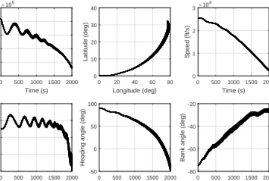
The optimal trajectories obtained without considering the no-fly zone constraint are firstly presented. Based on the ve-hicle dynamics, mission objectives and constraints illustrated in Section II, the results in the last population are shown in Fig.1 and Fig.2.
As can be observed from Fig.1 and Fig.2, the proposed multi-objective optimal control solver manages to generate state trajectories between the predetermined initial and final
conditions without violating path constraints. Therefore, the thermal and structural safety of the entry vehicle can be guaranteed, which is the prerequisite for the validity of an optimal control solver to spacecraft trajectory optimization problems. To effectively capture the true behaviour of the flight vehicle, a high density of mesh grids is required. However, the high density of nodes tends to have negative influences in terms of the evolution and convergence processes. One way to handle this problem is to introduce the lag equation as described in Eq.(8). The function of the lag equation is similar to a first-order filter, that can filter the control input signal and make the trend in the actual control history smoother. This is apparent in Fig.1 (see the bank angle profile).
Since all the trajectory in the final population are feasible solutions, the next step is to verify the pareto-optimality and improvement of the proposed algorithm over other multi-objective solvers. An attempt is made to compare the so-lutions obtained using the proposed method, MOPSO [41] and MOEA/D [21] approaches on maximizing final latitude versus minimizing heating pane. Non-optimal results may produce higher heat loads than necessary for a desired cross range. Fig.3 shows the Pareto fronts obtained by different evolutionary approaches investigated in this paper. As illus-trated in Fig.3, the improved NSGA-III algorithm generally preforms better than other multi-objective heuristic solvers for solving the multi-criteria trajectory planning problem, since the pareto set calculated by applying the proposed technique can cover the pareto front calculated using other heuristic algorithms. More precisely, the first front set (rank 1) obtained by the proposed algorithm contains 49 pareto-optimal solutions, whereas there are only 39 and 23 pareto-optimal solutions calculated using MOEA/D and MOPSO lying on the first front, respectively. In addition, the distribution of pareto fronts obtained using the extended NSGA-III is more uniform in the objective space. This is because the supply of a set of well-distributed reference points and the niching methodology in searching pareto-optimal solutions associated with every reference point have made the diversity preservation of obtained solutions more efficient and reliable.
J1 (Maximize cross range, deg)
29.5 30 30.5 31 31.5 32 32.5 33 J2
(Minimize total aerodynamic heating, KBtu)
105 110 115 120 125 130 135 Extended NSGA-III MOEA/D MOPSO
Fig. 3: Pareto front obtained via three solvers (Case 1)
Due to the randomness of evolutionary-based optimiza-tion methods in initializaoptimiza-tion, it is not enough to analyze the simulation results in only one trial. In order to eliminate the influences of randomness, this study has implemented three
TABLE III: Statistical boundary results (mission case 1)
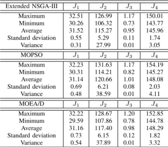
Extended NSGA-III 𝑒𝑟(𝑓 𝑡) 𝑒𝑉(𝑓 𝑡/𝑠) 𝑒𝛾(𝑑𝑒𝑔) Maximum 2773.92 240.88 0.95 Minimum 16.60 5.27 0.00 Average 1047.74 106.50 0.34 Standard deviation 786.57 64.43 0.26 MOPSO 𝑒𝑟(𝑓 𝑡) 𝑒𝑉(𝑓 𝑡/𝑠) 𝑒𝛾(𝑑𝑒𝑔) Maximum 2977.40 316.04 1.00 Minimum 24.18 19.49 0.00 Average 1313.51 127.52 0.50 Standard deviation 979.56 85.45 0.29 MOEA/D 𝑒𝑟(𝑓 𝑡) 𝑒𝑉(𝑓 𝑡/𝑠) 𝑒𝛾(𝑑𝑒𝑔) Maximum 2943.56 267.81 0.99 Minimum 29.27 12.03 0.00 Average 1169.23 162.53 0.39 Standard deviation 866.93 85.71 0.29 TABLE IV: Statistical objective results (mission case 1)
Extended NSGA-III 𝐽1 𝐽2 𝐽3 𝐽4 Maximum 32.51 126.99 1.17 150.01 Minimum 30.26 106.32 0.73 143.77 Average 31.52 115.27 0.95 145.96 Standard deviation 0.55 5.29 0.11 1.74 Variance 0.31 27.99 0.01 3.05 MOPSO 𝐽1 𝐽2 𝐽3 𝐽4 Maximum 32.23 131.63 1.17 154.19 Minimum 30.31 114.21 0.82 145.27 Average 31.14 120.66 1.01 148.08 Standard deviation 0.69 6.21 0.08 2.03 Variance 0.48 38.59 0.01 4.11 MOEA/D 𝐽1 𝐽2 𝐽3 𝐽4 Maximum 32.22 128.67 1.20 152.85 Minimum 29.59 107.86 0.78 144.78 Average 31.16 117.40 0.98 148.29 Standard deviation 0.73 6.15 0.12 1.82 Variance 0.54 37.89 0.01 3.32
evolutionary-based solvers to run each mission scenario in 20 trials independently. The statistical comparison of the solutions obtained in 20 trials is tabulated in Table.III and Table.IV. Specifically, the final boundary results are shown in Table.III, whereas the objective results are shown in Table.IV. It can be observed from Table.III that compared with other MOEA solvers, the proposed strategy tends to have a robust and stable behaviour in terms of achieving the final boundary conditions. Regarding the specific efficiency of the calculation, the average processing time for the optimization procedure is about 1h 12m (4331.2s). It is important to remark that for practical spacecraft guidance and control systems, the design of optimal flight trajectories is usually carried out offline. In addition, if parallel computing or high-performance computers can be implemented to optimize the flight path, this processing time can be further decreased.
D. Flight trajectory results with tighter path constraints
To further test the performance of the solver and con-straint handling strategy, another mission scenario (Case 2) which sets tighter requirements on the path constraints was carried out using the improved NSGA-III algorithm. In this case, the aerodynamic heating, dynamic pressure and load factor constraints are restricted to [ ˙𝑄𝑚𝑎𝑥, 𝑃𝑑𝑚𝑎𝑥, 𝑛𝑚𝑎𝑥𝐿 ] = [150,250,1.25], respectively. The time history of the optimiza-tion variable is plotted in Fig.4. Detailed results in terms of terminal error values and different objective function values are given in Table.V and Table.VI, respectively.
Time (s) 0 500 10001500 2000 Altitude (ft) ×105 0.5 1 1.5 2 2.5 3 Longitude (deg) 0 20 40 60 80 Latitude (deg) 0 10 20 30 40 Time (s) 0 500 100015002000 Speed (ft/s) ×104 0 1 2 3 Time(s) 0 500 10001500 2000
Flight path angle (deg)
-6 -4 -2 0 2 Time (s) 0 500 1000 15002000
Heading angle (deg)
-100 -50 0 50 100 Time (s) 0 500 100015002000
Bank angle (deg)
-80 -60 -40 -20
Fig. 4: Time history of states and controls (case 2)
Time (s) 0 500 1000 1500 2000 Q (BTU) 0 50 100 150 Time(s) 0 500 1000 1500 2000 Dynamic pressure (lb) 0 100 200 300 Time (s) 0 500 1000 1500 2000 Load factor -0.5 0 0.5 1 1.5 time (s) 0 500 1000 1500 2000 Atmosphre ρ ×10-4 0 0.5 1
Fig. 5: Time history of path constraints (case 2)
J1 (Maximize cross range, deg)
29.8 30 30.2 30.4 30.6 30.8 31 31.2 31.4 31.6 31.8 J2
(Minimize total aerodynamic heating, KBtu)
108 110 112 114 116 118 120 122 124 126 Extended NSGA-III MOEA/D MOPSO
Fig. 6: Pareto front obtained via three solvers (case 2)
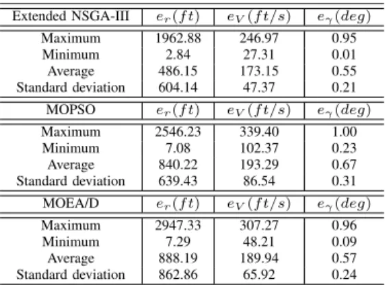
TABLE V: Statistical boundary results (mission case 2)
Extended NSGA-III 𝑒𝑟(𝑓 𝑡) 𝑒𝑉(𝑓 𝑡/𝑠) 𝑒𝛾(𝑑𝑒𝑔) Maximum 1962.88 246.97 0.95 Minimum 2.84 27.31 0.01 Average 486.15 173.15 0.55 Standard deviation 604.14 47.37 0.21 MOPSO 𝑒𝑟(𝑓 𝑡) 𝑒𝑉(𝑓 𝑡/𝑠) 𝑒𝛾(𝑑𝑒𝑔) Maximum 2546.23 339.40 1.00 Minimum 7.08 102.37 0.23 Average 840.22 193.29 0.67 Standard deviation 639.43 86.54 0.31 MOEA/D 𝑒𝑟(𝑓 𝑡) 𝑒𝑉(𝑓 𝑡/𝑠) 𝑒𝛾(𝑑𝑒𝑔) Maximum 2947.33 307.27 0.96 Minimum 7.29 48.21 0.09 Average 888.19 189.94 0.57 Standard deviation 862.86 65.92 0.24
TABLE VI: Statistical objective results (mission case 2)
Extended NSGA-III 𝐽1 𝐽2 𝐽3 𝐽4 Maximum 31.78 121.83 1.19 146.46 Minimum 30.61 110.70 0.84 142.23 Average 31.16 114.58 1.04 143.65 Standard deviation 0.35 3.31 0.07 0.93 Variance 0.12 10.98 0.01 0.86 MOPSO 𝐽1 𝐽2 𝐽3 𝐽4 Maximum 31.53 124.82 1.20 148.44 Minimum 29.81 109.88 0.92 142.01 Average 30.91 117.02 1.10 144.73 Standard deviation 0.45 3.55 0.08 0.94 Variance 0.21 12.61 0.01 0.89 MOEA/D 𝐽1 𝐽2 𝐽3 𝐽4 Maximum 31.71 125.20 1.25 148.32 Minimum 29.81 109.87 0.91 142.02 Average 30.95 115.25 1.05 144.60 Standard deviation 0.44 3.69 0.07 1.17 Variance 0.19 13.64 0.01 1.37
From Fig.4, the obtained state and control profiles are smooth enough and can vary in their tolerant set during the entire time history. It should be noted that one important factor that can have significant influences in the results is the atmospheric model 𝜌. Similarly with the result presented in Fig.2, the path constraint profiles, together with the 𝜌
profile, are displayed in Fig.5. From Fig.5, it is obvious that the dynamic pressure and load factor constraint values increase significantly as𝜌 increases. This phenomena affects the characteristic of the altitude, flight path angle and bank angle trajectories shown in Fig.1 and Fig.4. For example, after around 1500s, the altitude profile tends to be much smoother, which is mainly influenced by the flight path angle. This can be explained by the fact that the oscillations in the trajectory tend to make the dynamic pressure and load constraints becoming active. In order to decrease these two constraint values, the variance of the flight path angle should be decreased and this is mainly achieved by increasing the bank angle gradually.
According to the results shown in Table.V and Table.VI, the proposed solver can again achieve smaller final state errors and better objective results than other multi-objective algo-rithms. In addition, Fig.6 gives the Pareto fronts obtained by the three approaches on maximizing final latitude versus mini-mizing heating pane. Again, the improved NSGA-III performs better than its counterparts since the pareto front obtained using improved NSGA-III can cover fronts calculated using other methods and tends to be well-distributed. Specifically, for this case study, the improved NSGA-III algorithm obtains 37 pareto-optimal solutions in the first front set, while the first front set calculated using MOEA/D and MOPSO approaches only contains 34 and 18 elements, respectively. Therefore, although all the evolutionary-based solvers considered in this paper can be applied to generate feasible solutions for solving multi-objective trajectory optimization problems, the improved NSGA-III approach has quicker convergence speed and better global search ability under limited computational power. This further confirms that the designed method can have the ad-vantage over other evolutionary-based multi-discipline solvers considered in this paper.