This is a repository copy of
CME arrival time prediction using convolutional neural network
.
White Rose Research Online URL for this paper:
http://eprints.whiterose.ac.uk/149545/
Version: Accepted Version
Article:
Wang, Y., Liu, J. orcid.org/0000-0003-2569-1840, Jiang, Y. et al. (1 more author) (2019)
CME arrival time prediction using convolutional neural network. The Astrophysical Journal,
881 (1). 15. ISSN 0004-637X
https://doi.org/10.3847/1538-4357/ab2b3e
© 2019. The American Astronomical Society. This is an author-produced version of a paper
subsequently published in The Astrophysical Journal. Uploaded in accordance with the
publisher's self-archiving policy.
[email protected] https://eprints.whiterose.ac.uk/ Reuse
Items deposited in White Rose Research Online are protected by copyright, with all rights reserved unless indicated otherwise. They may be downloaded and/or printed for private study, or other acts as permitted by national copyright laws. The publisher or other rights holders may allow further reproduction and re-use of the full text version. This is indicated by the licence information on the White Rose Research Online record for the item.
Takedown
If you consider content in White Rose Research Online to be in breach of UK law, please notify us by
CME Arrival Time Prediction Using Convolutional Neural Network Yimin Wang,1, 2 Jiajia Liu,1 Ye Jiang,3 andRobert Erd´elyi1, 4
1Solar Physics and Space Plasma Research Center (SP2RC), School of Mathematics and Statistics The University of Sheffield, Sheffield S3 7RH, UK
2
School of Electrical Engineering, University of Jinan, Jinan 250022, China 3
Department of Computer Science, The University of Sheffield, Sheffield S1 4DP, UK 4
Department of Astronomy, E¨otv¨os Lor´and University, Budapest, P´azm´any P. s´et´any 1/A, H-1117, Hungary ABSTRACT
Fast and accurate prediction of the arrival time of Coronal Mass Ejections (CMEs) at the Earth is vital to minimize hazards caused by CMEs. In this paper, we use a deep learning framework, i.e. a convolutional neural network (CNN) regression model, to analyze transit times from the Sun to the Earth of 223 geo-effective CME events observed in the past 30 years. 90% of them were used to build the prediction model, and the rest 10% have been used for test purpose. Unlike previous studies on this topic, our proposed CNN regression model does not require manually selected features for model training, does not need time spent on feature collection, and can deliver predictions without deeper expert knowledge. The only input to our CNN regression model is the instances of the white-light observations of CMEs. The mean absolute error of the constructed CNN regression model is about 12.4 hours, which is comparable to the average performance of the previous studies on this subject. As more CME data are available, we expect the CNN regression model will reveal better results.
Keywords: Sun: coronal mass ejections (CMEs) — solar–terrestrial relations — Convolution Neural Network
1. INTRODUCTION
Coronal Mass Ejections (CMEs) are ejects of mass and magnetic flux from the Sun into the interplane-tary space (Lin and Forbes 2000). Generally, it takes CMEs one to five days to propagate from the Sun onto the Earth, which enables the prediction of their arrival times in advance become theoretically feasible. Once ar-riving at Earth, CMEs could cause severe disturbances to the terrestrial upper atmosphere, such as the magne-tosphere, and lead to violent geomagnetic storms (e.g., Gosling et al. (1991); Webb et al. (2000); Wang et al. (2002); Zhang et al. (2007); Chi et al. (2016)). These magnetic storms could cause potentially serious dam-ages to spacecrafts, modern communication systems, high-voltage power grids and oil or gas pipelines. Thus, fast, accurate and reliable prediction of CME arrival time at Earth is highly demanded by a range of indus-tries and other stakeholders, e.g. in security and defense sectors.
Corresponding author: Jiajia Liu
Zhao and Dryer (2014) reviewed the CME tran-sit time prediction models including empirical mod-els (Vandas et al. (1996); Brueckner et al. (1998); Gopalswamy et al. (2000); Gopalswamy et al. (2001); Wang et al.(2002);Zhang et al.(2003);Manoharan et al. (2004); Kim et al. (2007); Michalek et al. (2008)), ex-pansion speed model (Schwenn et al. 2005), drag-based models (Vrˇsnak(2001);Song(2010);Subramanian et al. (2012); Vrˇsnak et al. (2013)), physics-based models (Moon et al. (2002); Feng et al. (2009); Qin et al. (2009);Liu and Qin(2012)), and time-dependent MHD models (T´oth et al. (2012); Riley et al. (2013)), and claimed that no great gaps are found between their prediction capabilities and accuracies. The predictions yield in general about 10 hours of mean absolute error (MAE) for a large number of events.
In the past few years, machine learning meth-ods such as the Support Vector Machine (SVM) (Cortes and Vapnik 1995), fully-connected neural net-work (FCNN) (Hinton et al. 2006) and convolutional neural network (CNN) (Lecun et al. 1998) have been successfully applied to the analyses of several space weather forecasting problems. Li and Zhu (2013) used
FCNN for solar flare forecasting. Bobra and Ilonidis (2016) employed features derived from photospheric vector magnetic field data and X-ray flux data as the input to a SVM machine learning model to forecast whether an active region that produces large solar flares will also produce a CME, without considering CME transit times. McGregor et al. (2017) applied CNN to solar flare predictions. Yang et al.(2018) used FCNN to predict solar wind speeds at 1 AU.Huang et al. (2018) applied CNN to automatically extract forecasting pat-terns from magnetograms of active regions to predict C-, M- and X-class flares.
Despite applying machine learning techniques to solar flare predictions, not much effort has been devoted to applying machine learning to CME arrival/transit time predictions. Sudar et al.(2016) used a FCNN to analyze the CME transit time as a function of CME initial speed and central meridian distance that resulted in the MAE of about 11.6 hours. This 11.6-hour MAE is the average over ten MAEs with each MAE calculated from a ran-domly sampled testing dataset. Further, as the first step of our series of efforts in making space weather predic-tions, Liu et al. (2018) used 182 geo-effective (partial-)halo CMEs and built an SVM model to predict the CME arrival time, and obtained the MAE of 5.9 hours. This 5.9 hours is the best MAE of 100,000 MAEs with each MAE computed from a randomly sampled testing dataset. The above models used manually selected pa-rameters to form the input to the models, which: 1) usually is quite time-consuming to obtain from original observations, 2) could be biased because of the possi-bility of missed important parameters, and 3) requires specific CME-related expert knowledge for manual fea-ture selection. It is also worth noting that, here in this work, we will use k-fold cross validation approach (Mosteller and Tukey 1968) to examine the model per-formance, that obtains the average MAE of the predic-tion around 12.4 hours, which is the most popular way to be used in data mining. Compared with the validation methods inSudar et al.(2016) andLiu et al.(2018), the k-fold cross validation can result in a less optimistic or less biased estimate of the model performance, espe-cially when there is a limited number of samples (Kohavi (1995);Zhang and Yang(2015)). Further details about thek-fold cross validation are given in Section2.2
To this end, we use a CNN regression model to pre-dict the CME transit times. Our main contributions are that:
• This is the first time that the CNN method is ap-plied to the problem of CME arrival time predic-tion.
• The only input to train the model and deliver pre-dictions are directly observed images.
• Our proposed model eases the laborious dealing of manual features selection.
• The proposed model allows the lack of a deeper specific expert knowledge to perform the predic-tions.
• No matter what stage the evolution of a CME event is observed by the LASCO C2 coronagraph, once a new CME image is taken, its transit time to the Earth can be predicted immediately, and the prediction result can be obtained within a second. The rest of the paper is organized as follows. In Sec-tion2, we introduce the data source used in this study, and discuss the dataset prepared for the training and validation of our model. In Section 3, we describe the CNN algorithm, the configurations of our proposed CNN regression model, and the details of the model train-ing and validation. The validation results are then pre-sented in Section4, and the configurations of our model are compared with a baseline model and the pretrained Inception-ResNet-v2 model. Section5concludes the pa-per.
2. DATA 2.1. Data source
We have employed an approach analogue to the one in CAT-PUMA (Liu et al. 2018) in order to construct the dataset to be used in this research. In this section, let us now briefly recap the data extraction process for the built-up of the database to be used here.
A catalogue of all observed geo-effective CMEs since the beginning of the SOHO era, i.e. from 1996 to early 2018 was established by combining the following four CME databases: the Richardson and Cane list1
(Richardson and Cane 2010), the full halo CME list pro-vided by the University of Science and Technology of China2
(Shen et al. 2013), the George Mason Univer-sity CME/ICME list3
(Hess and Zhang 2017), and the CME Scoreboard by NASA4
. After removing duplicates, 276 geo-effective events were obtained. Different from Liu et al.(2018), where CMEs with angular width less than 90◦were removed, in this research, all CMEs with
no matter what their angular widths are now kept.
1
http://www.srl.caltech. edu/ACE/ASC/DATA/level3/icmetable2.htm
2
http://space.ustc.edu.cn/dreams/fhcmes/ index.php
3
http://solar.gmu.edu/heliophysics/index.php/GMU CME/ICME List
After obtaining a combined catalogue of geo-effective CMEs observed in the past two decades, the SOHO LASCO (Brueckner et al. 1995b) C2 white-light corona observations, from 10 minutes before up to 2 hours after the onset times of the events, were acquired. The LASCO C2 coronagraph measures the white-light corona from 1.5 to 5 solar radii, usually allowing the detection of CMEs in their early stages before travel-ling into the interplanetary space. For each CME event, we used the“lasco readfits.pro” module of theSSWIDL
package to enquire the downloaded fits files. Next, from each image file, the first downloaded image of the cor-responding event was subtracted to generate a series of “base-difference” images to be rescaled to a range of 0 to 255 with a data range of -1000 to 1000 DN. All images were further manually checked and images with no or poor CME observations were then removed.
After carrying out all the above procedures, one ob-tains 1122 base-difference images of 223 geo-effective CMEs detected in the period of 1997 to 2017.
2.2. Data preprocessing
In the dataset described above, the number of images that are contained in one event ranges from one to ten. All the images from an event are categorized into one iso-lated folder, thus there are 223 folders. For each event, the CME arrival time to the Earth is saved as a text file. Each image file name is the time of its observation. Therefore, the transit time of a CME can be calculated by subtracting the arrival time by the time of observa-tion of its corresponding image file name. In order to alleviate the computational cost, the images, which are originally 1024 × 1024 pix2
, are re-scaled to a smaller resolution: 256× 256 pix2
. The image pixels are then scaled down by a factor of 255, i.e. they are transformed from the range [0, 255] to [0, 1]. This normalization step is to make the images contribute more evenly to the total loss function of the model. The CME images, although saved in a three-channel color mode, i.e. in RGB format, are actually grayscale images. Therefore, all the obtained images are then converted from RGB to grayscale.
Next, a validation method is used to estimate the per-formance of a model on unseen data. That is, we esti-mate how the model performs when used to make pre-dictions on a testing dataset that are not used during the training of the model. There are various ways to separate a dataset into training and testing sets. A com-mon way is to simply divide the dataset into two groups and assign a smaller portion, typically 20%, to the test-ing set, and use the remaintest-ing data for the traintest-ing set. Another popular approach is thek-fold cross-validation
(Mosteller and Tukey 1968). The general procedure is as follows: 1) shuffle the dataset randomly, 2) split the dataset into k groups, 3) for each unique group, take it as a hold out or a testing dataset, and take the remaining groups as a training dataset, and 4) fit a model with the training dataset and validate it with the testing dataset. Therefore, the validation method of dividing the entire dataset into two groups is simply an equivalent of one fold of thek-fold cross validation. In Section1, we have already mentioned thatk-fold cross validation can result in a less optimistic or less biased estimate of the model performance. This is because, with k-fold cross valida-tion, each sample of the entire dataset is used in the testing set, which avoids easily to be biased by lucky or unlucky selection or cherry-picked testing set as in an-other validation methods. Kohavi(1995) recommended that the 10-fold cross validation is better at reducing variance and bias, and is thus commonly used in ma-chine learning. For applying the 10-fold cross validation method in this work, we need to guarantee that images belonging to the same event are given to one group only, i.e. they must not be separated, otherwise there will be correlated images between the training and testing datasets. To this end, we shuffle all the 223 events ran-domly, which are then splitted into ten groups with each group containing approximately 22 events, i.e. 10% of all the 1122 images.
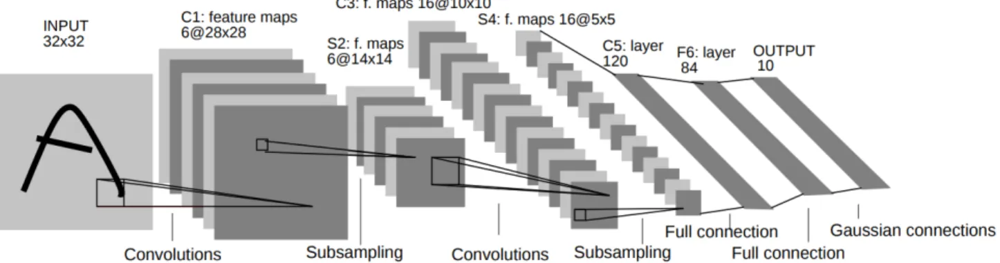
3. CONVOLUTIONAL NEURAL NETWORK The area of neural networks is inspired by the goal of modelling the connectivity of neurons in the human brain. These networks turn out to be well-suited to model high level abstractions across a wide range of dis-ciplines. Figure 1 shows the first standard CNN archi-tecture, namely the LeNet-5 (Lecun et al. 1998).
3.1. Basic CNN components
A simple CNN is a sequence of layers, where each layer transforms one volume of tensor or activation to another through a differentiable function. Different layer types used in a typical CNN primarily include:
• Convolutional Layer: The convolutional layer acts as a filter for feature extraction from images. Figure 1 shows the first CNN, LeNet-5, that consists of sev-eral feature maps, which are responses to the filters in the presence of certain kinds of features with each filter learning to look for different features from the input. As we go deeper through the network, i.e. go through more convolutional layers, we obtain feature maps that represent more and more abstract features.
• Pooling Layer: The extracted feature maps are then passed to the pooling layer, which sub-samples its
in-Figure 1. The architecture of LeNet-5. Each plane is a feature map, and a neuron is a set of units whose weights are constrained to be identical for a feature map (Lecun et al. 1998).
puts while preserving the most important information in them. The pooling layer can reduce the dimensions of the feature maps and increase robustness of the feature extraction. Two typical pooling schemes are average pooling (Wang et al. 2012) and max pooling (Boureau et al. 2010).
• Fully-connected Layer (also called dense layer): The fully-connected layer takes the high-level features from the previous layer and translates them into pre-dicted values in terms of regression problems. Since each input sample can only be formatted onto one-dimensional data for feeding into the fully-connected layer, there is no spatial information preserved in this layer.
Figure2 depicts the information flow through a neu-ron. The training dataset is given in pairs of (xi, yi).
CNN acquires an image (xi) through a small window,
e.g. 3 × 3 pix2
, which is a 3 × 3 weights matrix (W), called a filter or neuron or kernel. The weights W = (w0, w1, w2, ...) are initialized as random numbers
and are the learnable parameters. During forward prop-agation, a feature map or activation map, which is a matrix, is formed by sliding the filter (W) over an im-age (xi) for computing the dot product, adding the bias
(b), and applying the non-linearity or activation function f:
y=f(W x+b). (1) Here, xand y represent the input and output tensors, respectively. The input tensor could be an input image or a feature map from a previous layer. The activation function, f, enables the neurons to represent a com-plex non-linear dynamic system. Without the activation function, the result of a neural network is just linear combinations of input parameters. By a similar mecha-nism, the dense layer computes the predicted value ˆyi,
though its associated filter (W) is a one-dimensional vec-tor for each feature instead of a two-dimensional win-dow. The loss function L is the compatibility between
the predicted value ˆyi and the labelyi. The
regulariza-tion loss is just a funcregulariza-tion of the weights that is used to control over-fitting. At this point, the gradient descent optimization algorithm is used to minimize the loss via updating the NN weights and bias through backprop-agation based on the training dataset. This training process continues iteratively until it converges.
Figure 2. The information flow of a neuron (Li 2018)
3.2. The configuration of our proposed CNN regression model
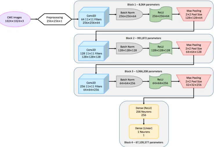
The schematic diagram of our proposed CNN regres-sion model is shown in Figure3. Parameters of the CNN can be learned automatically from the input data during the training process. However, some hyperparameters need to be set up before training (Bengio 2012). One type of such hyperparameters is called the model hy-perparameters, which specify the structure of the CNN model. The other type, the so-called training hyperpa-rameters, determine how the model is trained.
Observations show that, the expression ability of a NN is enhanced as the size of it increases, which includes the depth and width of the network. While as the size of a NN increases, more training data is required to optimize the parameters of the model, and the memory consump-tion increases as well. Therefore, in our experiments, we increase the model size until the performance of the model does not improve anymore, or the computational cost is too high to afford.
Figure 3. The schematic diagram of our CNN regression model. We determined the configurations through trial and error and tailored them to minimize the MSEs.
A number of experiments have been conducted for de-termining the structure of the CNN regression model. Several typical configurations of CNNs are introduced for aiding to explain how the proposed structure is de-veloped: 1) a convolutional layer is normally followed by a batch normalization (BN), an activation function and a max pooling; 2) the number of neurons in a layer is in powers of 2, starting from 32; 3) the typical numbers of window size are 3, 5, 7, 11. These typical config-urations are used mainly for effectively finding a good hyperparameter choice compared to try the sizes with a unit increment each time. In the 10-fold cross vali-dation, for each individual testing set, we evaluate the performance of the model by calculating the MAE of each CME image. For the testing set, with a total num-ber ofM images, the MAE is calculated as follows:
MAE = 1 M M X m=1 |ym−yˆm|. (2)
Here,ymis the true target value, and ˆymis the predicted
target value. The subscriptmrepresents themth
input sample.
Convolutional layers are used to automatically extract features from input data, of which the depth and width directly affect the prediction accuracy. For determin-ing the appropriate number of convolutional layers, five main steps are taken. At each step, the depth and width of dense layers are also experimented in a similar man-ner. The five steps are shown as follows:
1. Models are composed of only one convolutional layer, stacked by dense layers. The numbers of neurons for the convolutional layer are 32 or 64. Going beyond 64 neurons for the first layer costs too much computational resources. All the models from the first stage result in the MAEs 13.2-13.5 hours.
2. One more convolutional layer is added. Several combinations of numbers of neuron for these two convolutional layers are evaluated, e.g. 32 or 64 neurons for both convolutional layers, or 64 for the first convolutional layer and 128 for the sec-ond one. The MAEs of the two-convolutional-layer model decreased to 13.0-13.2 hours, with an
ex-ception when the window size is 11×11 pix2
, the MAE achieves 12.5 hours. It seems the 11×11 pix2
window size is more suitable for manipulating the CME images.
3. There are three convolutional layers followed by dense layers at this step. When the window size is 11×11 pix2
, the MAEs varied between 12.4-12.6 hours. The model structure that reaches the best performance is shown in Figure 3. For other win-dow sizes, the MAEs are between 12.5-12.8 hours. A larger window size of 15×15 pix2
is also ex-amined, and it produces the MAE of 12.8 hours, which is not as good as the 11×11 pix2
one. These experiments further confirm that 11×11 pix2
is more suitable for the CME dataset.
4. When the number of convolutional layers increases to four and five, the MAEs are always stuck at 12.7-13.1 hours, implying that noise may be intro-duced due to insufficient training data for these depths of the network.
5. After taking the best CNN model from step 3, CNN structures with/without BN and max pool-ing layers, and positions of BN before/after the activation functions are then evaluated. Training hyperparameters are also explored for the chosen model, which includes batch size, activation func-tion, and learning rate etc. Finally, the CNN re-gression model is determined as shown in Figure 3
The activation function employed in our CNN re-gression model is the rectified linear unit (ReLU) (Nair and Hinton 2010), and a linear function is ap-plied only to the last layer, which is able to output the full range of values of the target variable. For a better generalization, BN (Ioffe and Szegedy 2015) is applied after the convolutional layers, which is a regularization technique used to convert the distributions of all input features to have zero mean and one standard deviation. In this way, the later layer can treat all features equally, and thus reduce the oscillations of the optimizer when approaching the minimum point. The model is trained to minimize the mean-squared error (MSE) loss func-tion using Adam optimizer (Kingma and Ba 2014) with a learning rate of 0.001. For the training set with a total number of N images, MSE is calculated as follows:
MSE = 1 N N X n=1 (yn−yˆn) 2 , (3)
where yn is the true target value, and ˆyn is the
pre-dicted target value. The subscriptnrepresents the nth
input sample. MSE is commonly used in solving regres-sion problems because it can deliver better result than other loss functions tested while developing our CNN regression model. In the training process, each of the 10-fold is trained 500 epochs and the model weights of each fold is determined from the epoch that generates the minimal MSE. The model error is then obtained by averaging the 10-fold MSEs. We determined the con-figurations through trial and error and tailored them to minimize the MSEs. The batch size used in the training process is 64.
The number of trainable parameters of a two-dimensional convolutional layer (Conv2D) is calculated by the filter height times the filter width times num-ber of feature maps (or channels) from the previous layer as the number of weights of one filter, plus one bias for this filter, and then times the number of filters for all filters. For example, assuming that the input image has 256 pixels in height, 256 pixels in width and 1 channel since it has been converted to grayscale. The Conv2D in the first layer of our CNN regression model has 64 filters with each filter 11×11 weights. The number of trainable parameters of this Conv2D is (11×11×1 + 1)×64 = 7808. A BN computes two trainable parameters and two non-trainable parameters per feature map on the previous layer, which makes the BN in the first layer having 4×64 = 256 parameters with 128 trainable and 128 non-trainable parameters, respectively. ReLU and max pooling do not have any parameters. Therefore, in total, the first layer contains 7808 + 256 = 8064 parameters. The number of train-able parameters of a dense layer is computed by the number of input plus one bias, and then times the num-ber of neurons. For example, the first dense layer in our model has 256 neurons, and its number of input is 32×32×256 = 262,144, which makes its number of trainable parameters (262,144 + 1)×256 = 67,109,120.
The code is available at https://github.com/ yiminking/CME-CNN. The implementation of our CNN regression model is built using Keras (Chollet et al. 2015), which is a high-level API of TensorFlow (Abadi et al. 2015). TensorFlow is an open source software library developed by Google Brain team 5
, and it is one of the most popular infrastructure for running machine learning algorithms.
4. EXPERIMENTAL RESULT AND ANALYSIS
A deep learning approach is proposed for CME arrival time prediction, which is able to automat-ically extract predicting features from the
light observations of CMEs. The average MAE over ten testing sets is 12.4 hours varying between 10.1 hours and 16.2 hours.
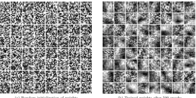
During the training process, weights in the convolu-tional layers are iteratively adjusted to minimize the er-ror between the predicted and the true arrival time of a CME. Taking the first convolutional layer in the CNN model for example, we aim to understand how the model comprehends the CME images, and how different model structures affect the prediction accuracy. The weights of 64 neurons are initialized by random numbers at the start of the training process as shown in Figure 4(a), and the averaged MAE of the 10-fold cross validation is 65.8 hours ranging from 55.2 to 80.5 hours before the training. In Figure4(b), the weights are adjusted to the patterns after the model is trained for 500 epochs, which look at a CME image from different aspects.
In order to understand how the model structures af-fect the prediction accuracy, the feature maps from four different models are compared as shown in Figure 5. The training hyperparameters and dense layer scheme are kept the same for these four models. Figure 5(a) is the original input CME image. This image contains at least 4 different features: the black disk as the Sun, the white structure as the CME, the black structure between the CME and the Sun as the CME when it ap-peared in the LASCO C2 FOV for the first time, and the vast black background with noises. Figure 5(b) is generated by a model with only one convolutional layer with 32 neurons and window size 3×3 pix2
. This model produced the worst performance across all of our ex-periments, of which the averaged 10-fold MAE is 13.5 hours. This could be expected as we can see from Fig-ure5(b) that, not a single filter successfully distinguish between the above four features. The Sun, the CME and the background were almost mixed together with similar brightness in all filters. Figure5(c) is generated by a two-convolutional-layer model with an improved MAE of around 13.0 hours. Filters in this model start to look at the desired locations, but with only one filter (at the second row and second column) makes the CME brighter enough than the solar disk and the background. Figure 5(d) is from a three-convolutional-layer model with halved number of neurons compared with the pro-posed model and the window size 3×3 pix2
. Com-pared to the two-convolutional-layer model, more filters in this three-convolutional-layer model successfully dis-tinguish the desired features. Figure 5(e) is generated by the proposed CNN regression model, which shows clear concentration on the CME. Interestingly, for fil-ters that successfully distinguish between the CME and the background, the contrasts between the CME and
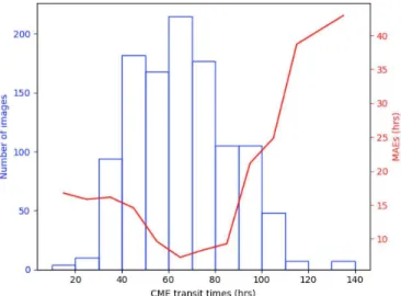
the background are higher in the proposed model than in the three-convolutional-layer model. Meanwhile, the background is also less noisy. These findings mean that proposed model performs better in separating the CME from the background and ignoring the background noise. Figure6depicts the distribution of CME transit times against their corresponding MAEs for all the testing data. The bins are ten-hour wide. We can see that the more the image samples fall in a transit time range, the smaller the MAE, i.e. the more accurate its pre-diction. When the transit times are in the range of 60 to 70 hours, there are the most numbers of images, i.e. 215, and its MAE is just 7.3 hours. It needs to be noted that, 1122 images are considered to be a small dataset for deep learning methods. Due to their intrinsic prop-erties, deep learning approaches can learn the features of training data better when there is a sufficient amount of them. If more training data are available, the CNN regression model would yield much better results.
Figure 7 depicts the distribution of the MAEs for all the testing samples. The bins are four-hour wide. The figure shows that 60% of the images are contained in the first three bins, i.e. of which the predicted transit times are smaller than 12 hours.
In the ideal case, the correlation coefficients between the predicted and the actual transit times should be equal to 1, i.e. as marked by the blue dashed line in Figure8. The black dots demonstrate the transit times from all the testing samples. Despite several outliers, the agreement with the mean correlation coefficient (cor-rcoef) over the ten folds of 0.58 ranging between 0.35 to 0.83 looks satisfactory for the majority of the dots.
Out of the studied 223 events, the arrival times of 59 events have been predicted by various earlier mod-els available via the NASA CME Scoreboard. Figure9 shows a comparison of the prediction error between our model and these alternative models on these 59 events. The prediction error of our model on an event is the MAE of predictions made on all images used for one event, and the prediction error of the earlier models is the MAE of all available predictions at the NASA CME Scoreboard on the same event. It turns out that, in 38 (∼64.4%) events, our model gives a smaller prediction error than that of the average of the traditional models. For all these 59 events, the average prediction error of our model is about 12.6 hours, while the average pre-diction error of the studied traditional models is about 15.4 hours.
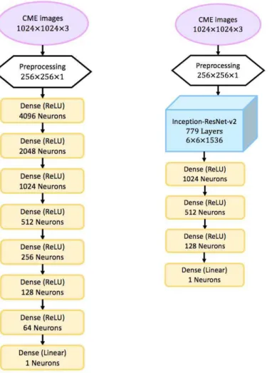
In our experiments, we also compared the proposed CNN regression model with an FCNN and the state-of-the-arts Inception-ResNet-v2 (Szegedy et al. 2016) models as shown in Figure10. We trained and validated
(a) Random initialization of weights (b) Trained weights after 500 epochs
Figure 4. Variation of the weights of the first convolutional layer before and after training.
Figure 5. Feature maps of the first convolutional layer of four model architectures. the CME dataset using an FCNN model with eight
layers as a baseline. The pretrained Inception-ResNet-v2 model was trained using the well-known ImageNet
dataset6
, meaning a reasonable number of features be-ing extracted from the ImageNet dataset that are then
Figure 6. The distribution of CME transit times and their corresponding MAEs for all the testing samples.
Figure 7. The distribution of MAEs for all the testing sam-ples.
Methods MAE corrcoef TP
FCNN 26.03 -0.01 279,625,729
Inception-ResNet-v2 13.10 0.55 56,440,673 CNN regression 12.42 0.58 72,074,652 Table 1. Comparison of the proposed CNN regression model with other commonly used approaches. MAE - Mean Abso-lute Error, corrcoef - correlation coefficient, TP - number of Trainable Parameters.
saved in the kernels of the Inception-ResNet-v2 model. In order to use the Inception-ResNet-v2 model in regres-sion tasks, we removed its top fully-connect layer which is used for classification problems, and attached another four fully-connected layers tailored for regression tasks.
Figure 8. Observed and predicted transit times of each image in the testing set. The blue dashed line depicts the case when the predicted transit hours equal the real ones, and the red dashed lines show the deviation from the blue line.
0 10 20 30 40 50 60
Average Prediction Error by Other Models (hrs) 0 10 20 30 40 50 60 Pr ed ic ti on E rr or b y O ur M od el ( hr s) 64.4% 35.6%
Figure 9. The prediction error calculated by our CNN re-gression model versus the average of the traditional methods. The blue dashed line indicates when the prediction error from our model is the same with that of the average of the tradi-tional models.
The comparison of the results is demonstrated in Ta-ble 1. The FCNN model has a testing MAE of 26.0 hours varying between 20.0-34.4 hours, and its correla-tion coefficient is only -0.01. This much worse result
Figure 10. The structure of the FCNN model (left) and the Inception-ResNet-v2 regression model (right). We determined the configurations of these two models through trial and error and tailored them to minimize the MSEs.
of FCNN compared with the CNN regression model is expected, because FCNN is not capable of extracting features from images. We have already mentioned in Section 3.1 that any dimension of input data has to be flattened to one-dimension before feeding to a fully-connected layer, therefore, no spatial information can be preserved. FCNN has trainable parameters about 4 times of the CNN regression model. The ImageNet dataset is composed of 1000 classes that are commonly seen in human life, e.g. animals and electronics, but it does not contain images similar to that of the CMEs. Therefore, even though the Inception-ResNet-v2 model has been pretrained, it does not defeat the CNN regres-sion model.
5. CONCLUSION
In this work, we have applied a CNN regression model to predict CME transit times using 1122 CME images observed by the SOHO LASCO C2 corograph (Brueckner et al. 1995a) from 223 events as the input data. The output is their corresponding transit times
estimated to be needed to propagate from the Sun to the Earth. The MAE over the entire sample is about 12.4 hours, which is very similar to that of the average performance of previous studies on the same subject. Due to the intrinsic properties of CNNs, more training samples can result in much better results, whereas 1122 images are considered to be a small size of dataset for the method of deep learning.
The most important benefit of our proposed CNN model is that it is not necessary to select features man-ually, which is usually rather time consuming, requires specific expertise, and can lead to failure of tasks if in-appropriate features are selected. Secondly, feature data collection, which is a redundant work and normally costs tens of hours of running time, is not necessary in our work. On the contrary, the only input to our CNN re-gression model is the instances of the white-light obser-vations of CMEs. Another benefit is, similar to FCNNs, that in our model it is not necessary to specify the empir-ical function or hyper-surface of mapping between input and output data.
The employed CNN regression model, as demon-strated in this work, only predicts the transit time for a CME that can finally arrive at the Earth, and it does not predict whether a CME will actually hit the Earth or not. The latter is another very important research task in space weather prediction. Therefore, the first follow-up step of our future work, would be to predict whether a CME can indeed arrive at the Earth using a much wider range of CME dataset, i.e. using all the CME events listed in the SOHO LASCO CME Catalog (Gopalswamy et al. 2009). Next, one needs to be reminded that, although CNN models are good at extracting features from images, they are not capable of dealing with time sequence data, i.e. CNN models treat images as isolated individuals without considering inter-relationships of the images. As the second step of our future work, we will therefore apply the deep learning approaches that can take evolutionary properties of the
CMEs image sequences into account, which may further improve the accuracy of CME arrival predictions.
ACKNOWLEDGEMENT
The SOHO LASCO CME catalog is generated and maintained at the CDAW Data Center by NASA and The Catholic University of America in cooperation with the Naval Research Laboratory. SOHO is a project of international cooperation between ESA and NASA. YW thanks for the warm hospitality and support re-ceived as an MSRC Visiting Research Fellow while car-rying out this research at the Solar Physics and Space Plasma Research Centre (SP2RC), School of Mathemat-ics and StatistMathemat-ics (SoMaS), The University of Sheffield. JL and RE are grateful to STFC (UK), grant number ST/M000826/1, and The Royal Society for their sup-port. We also acknowledge the use of a Titan Xp GPU kindly donated by the NVIDIA Corporation.
REFERENCES Abadi, M., Agarwal, A., Barham, P., Brevdo, E., Chen, Z.,
Citro, C., Corrado, G. S., Davis, A., Dean, J., Devin, M., Ghemawat, S., Goodfellow, I., Harp, A., Irving, G., Isard, M., Jia, Y., Jozefowicz, R., Kaiser, L., Kudlur, M., Levenberg, J., Man´e, D., Monga, R., Moore, S., Murray, D., Olah, C., Schuster, M., Shlens, J., Steiner, B., Sutskever, I., Talwar, K., Tucker, P., Vanhoucke, V., Vasudevan, V., Vi´egas, F., Vinyals, O., Warden, P., Wattenberg, M., Wicke, M., Yu, Y., and Zheng, X. (2015). TensorFlow: Large-scale machine learning on heterogeneous systems. Software available from tensorflow.org.
Bengio, Y. (2012). Practical recommendations for gradient-based training of deep architectures. CoRR, abs/1206.5533.
Bobra, M. G. and Ilonidis, S. (2016). Predicting coronal mass ejections using machine learning methods. The Astrophysical Journal, 821(2):127.
Boureau, Y.-L., Ponce, J., and LeCun, Y. (2010). A theoretical analysis of feature pooling in visual recognition. InProceedings of the 27th International Conference on International Conference on Machine Learning, ICML’10, pages 111–118, USA. Omnipress. Brueckner, G. E., Delaboudiniere, J.-P., Howard, R. A.,
Paswaters, S. E., St. Cyr, O. C., Schwenn, R., Lamy, P., Simnett, G. M., Thompson, B., and Wang, D. (1998). Geomagnetic storms caused by coronal mass ejections (CMEs): March 1996 through June 1997.
Geophys. Res. Lett., 25:3019–3022.
Brueckner, G. E., Howard, R. A., Koomen, M. J., Korendyke, C. M., Michels, D. J., Moses, J. D., Socker, D. G., Dere, K. P., Lamy, P. L., Llebaria, A., Bout, M. V., Schwenn, R., Simnett, G. M., Bedford, D. K., and Eyles, C. J. (1995a). The large angle spectroscopic coronagraph (lasco). Solar Physics, 162(1):357–402. Brueckner, G. E., Howard, R. A., Koomen, M. J.,
Korendyke, C. M., Michels, D. J., Moses, J. D., Socker, D. G., Dere, K. P., Lamy, P. L., Llebaria, A., Bout, M. V., Schwenn, R., Simnett, G. M., Bedford, D. K., and Eyles, C. J. (1995b). The Large Angle Spectroscopic Coronagraph (LASCO). Sol. Phys., 162(1-2):357–402. Chi, Y., Shen, C., Wang, Y., Xu, M., Ye, P., and Wang, S.
(2016). Statistical Study of the Interplanetary Coronal Mass Ejections from 1995 to 2015. SoPh, 291:2419–2439. Chollet, F. et al. (2015). Keras. https://github.com/
fchollet/keras.
Cortes, C. and Vapnik, V. (1995). Support-vector networks. Machine Learning, 20(3):273–297.
Feng, X. S., Zhang, Y., Sun, W., Dryer, M., Fry, C. D., and Deehr, C. S. (2009). A practical database method for predicting arrivals of “average” interplanetary shocks at earth. Journal of Geophysical Research: Space Physics, 114(A1).
Gopalswamy, N., Lara, A., Lepping, R. P., Kaiser, M. L., Berdichevsky, D., and St. Cyr, O. C. (2000).
Interplanetary acceleration of coronal mass ejections.
Gopalswamy, N., Lara, A., Yashiro, S., Kaiser, M. L., and Howard, R. A. (2001). Predicting the 1-au arrival times of coronal mass ejections. Journal of Geophysical Research: Space Physics, 106(A12):29207–29217. Gopalswamy, N., Yashiro, S., Michalek, G., Stenborg, G.,
Vourlidas, A., Freeland, S., and Howard, R. (2009). The SOHO/LASCO CME Catalog. Earth Moon and Planets, 104:295–313.
Gosling, J. T., McComas, D. J., Phillips, J. L., and Bame, S. J. (1991). Geomagnetic activity associated with earth passage of interplanetary shock disturbances and coronal mass ejections. Journal of Geophysical Research: Space Physics, 96(A5):7831–7839.
Hess, P. and Zhang, J. (2017). A Study of the
Earth-Affecting CMEs of Solar Cycle 24. SoPh, 292:80. Hinton, G. E., Osindero, S., and Teh, Y.-W. (2006). A fast
learning algorithm for deep belief nets. Neural Comput., 18(7):1527–1554.
Huang, X., Wang, H., Xu, L., Liu, J., Li, R., and Dai, X. (2018). Deep learning based solar flare forecasting model. i. results for line-of-sight magnetograms. The Astrophysical Journal, 856(1):7.
Ioffe, S. and Szegedy, C. (2015). Batch normalization: Accelerating deep network training by reducing internal covariate shift. CoRR, abs/1502.03167.
Kim, K.-H., Moon, Y.-J., and Cho, K.-S. (2007). Prediction of the 1-au arrival times of cme-associated interplanetary shocks: Evaluation of an empirical interplanetary shock propagation model. Journal of Geophysical Research: Space Physics, 112(A5). Kingma, D. P. and Ba, J. (2014). Adam: A method for
stochastic optimization. CoRR, abs/1412.6980. Kohavi, R. (1995). A study of cross-validation and
bootstrap for accuracy estimation and model selection. InProceedings of the 14th International Joint Conference on Artificial Intelligence - Volume 2, IJCAI’95, pages 1137–1143, San Francisco, CA, USA. Morgan Kaufmann Publishers Inc.
Lecun, Y., Bottou, L., Bengio, Y., and Haffner, P. (1998). Gradient-based learning applied to document recognition.
Proceedings of the IEEE, 86(11):2278–2324.
Li, F. (2018). Optimization: Stochastic gradient descent.
https://cs231n.github.io/optimization-1/#opt3. Li, R. and Zhu, J. (2013). Solar flare forecasting based on
sequential sunspot data. Research in Astronomy and Astrophysics, 13(9):1118.
Lin, J. and Forbes, T. G. (2000). Effects of reconnection on the coronal mass ejection process. Journal of
Geophysical Research, 105(A2):2375–2392.
Liu, H.-L. and Qin, G. (2012). Using soft x-ray observations to help the prediction of flare related interplanetary shocks arrival times at the earth. Journal of Geophysical Research: Space Physics, 117.
Liu, J., Ye, Y., Shen, C., Wang, Y., and Erd´elyi, R. (2018). A new tool for cme arrival time prediction using machine learning algorithms: Cat-puma. The Astrophysical Journal, 855(2):109–118.
Manoharan, P. K., Gopalswamy, N., Yashiro, S., Lara, A., Michalek, G., and Howard, R. A. (2004). Influence of coronal mass ejection interaction on propagation of interplanetary shocks. Journal of Geophysical Research (Space Physics), 109:A06109.
McGregor, S., Dhuri, D., Berea, A., and Munoz-Jaramillo, A. (2017). FlareNet: A Deep Learning Framework for Solar Phenomena Prediction. InNIPS Workshop on Deep Learning for Physical Sciences, Long Beach. Michalek, G., Gopalswamy, N., and Yashiro, S. (2008).
Space weather application using projected velocity asymmetry of halo cmes. Solar Physics, 248(1):113–123. Moon, Y.-J., Dryer, M., Smith, Z., Park, Y. D., and Cho,
K. S. (2002). A revised shock time of arrival (stoa) model for interplanetary shock propagation: Stoa-2.
Geophysical Research Letters, 29(10):28–1–28–4. Mosteller, F. and Tukey, J. W. (1968). Data analysis,
including statistics. In Lindzey, G. and Aronson, E., editors,Handbook of Social Psychology, Vol. 2. Addison-Wesley.
Nair, V. and Hinton, G. E. (2010). Rectified linear units improve restricted boltzmann machines. InProceedings of the 27th International Conference on International Conference on Machine Learning, ICML’10, pages 807–814, USA. Omnipress.
Qin, G., Zhang, M., and Rassoul, H. K. (2009). Prediction of the shock arrival time with SEP observations. Journal of Geophysical Research (Space Physics), 114:A09104. Richardson, I. G. and Cane, H. V. (2010). Near-Earth
Interplanetary Coronal Mass Ejections During Solar Cycle 23 (1996 – 2009): Catalog and Summary of Properties. Sol. Phys., 264(1):189–237.
Riley, P., Linker, J. A., and Miki´c, Z. (2013). On the application of ensemble modeling techniques to improve ambient solar wind models. Journal of Geophysical Research: Space Physics, 118(2):600–607.
Schwenn, R., Dal Lago, A., Huttunen, E., and Gonzalez, W. D. (2005). The association of coronal mass ejections with their effects near the earth. Annales Geophysicae, 23(3):1033–1059.
Shen, C., Liao, C., Wang, Y., Ye, P., and Wang, S. (2013). Source Region of the Decameter-Hectometric Type II Radio Burst: Shock-Streamer Interaction Region. SoPh, 282:543–552.
Song, W. B. (2010). An analytical model to predict the arrival time of interplanetary cmes. Solar Physics, 261(2):311–320.
Subramanian, P., Lara, A., and Borgazzi, A. (2012). Can solar wind viscous drag account for coronal mass ejection deceleration? Geophysical Research Letters, 39(19). Sudar, D., Vrˇsnak, B., and Dumbovi´c, M. (2016).
Predicting coronal mass ejections transit times to earth with neural network. Monthly Notices of the Royal Astronomical Society, 456(2):1542–1548.
Szegedy, C., Ioffe, S., and Vanhoucke, V. (2016).
Inception-v4, inception-resnet and the impact of residual connections on learning. CoRR, abs/1602.07261. T´oth, G., van der Holst, B., Sokolov, I. V., De Zeeuw,
D. L., Gombosi, T. I., Fang, F., Manchester, W. B., Meng, X., Najib, D., Powell, K. G., Stout, Q. F., Glocer, A., Ma, Y.-J., and Opher, M. (2012). Adaptive
numerical algorithms in space weather modeling.
Journal of Computational Physics, 231:870–903.
Vandas, M., Fischer, S., Dryer, M., Smith, Z., and Detman, T. (1996). Parametric study of loop-like magnetic cloud propagation. Journal of Geophysical Research: Space Physics, 101(A7):15645–15652.
Vrˇsnak, B. (2001). Deceleration of coronal mass ejections.
Solar Physics, 202(1):173–189.
Vrˇsnak, B., ˇZic, T., Vrbanec, D., Temmer, M., Rollett, T., M¨ostl, C., Veronig, A., ˇCalogovi´c, J., Dumbovi´c, M., Luli´c, S., Moon, Y.-J., and Shanmugaraju, A. (2013). Propagation of Interplanetary Coronal Mass Ejections: The Drag-Based Model. SoPh, 285:295–315.
Wang, T., Wu, D. J., Coates, A., and Ng, A. Y. (2012). End-to-end text recognition with convolutional neural networks. InProceedings of the 21st International Conference on Pattern Recognition (ICPR2012), pages 3304–3308.
Wang, Y. M., Ye, P. Z., Wang, S., Zhou, G. P., and Wang, J. X. (2002). A statistical study on the geoeffectiveness of Earth-directed coronal mass ejections from March 1997 to December 2000. Journal of Geophysical Research (Space Physics), 107:1340.
Webb, D. F., Cliver, E. W., Crooker, N. U., Cry, O. C. S., and Thompson, B. J. (2000). Relationship of halo coronal mass ejections, magnetic clouds, and magnetic storms. J. Geophys. Res., 105:7491–7508.
Yang, Y., Shen, F., Yang, Z., and Feng, X. (2018). Prediction of solar wind speed at 1 au using an artificial neural network. Space Weather, 16.
Zhang, J., Dere, K. P., Howard, R. A., and Bothmer, V. (2003). Identification of solar sources of major geomagnetic storms between 1996 and 2000. The Astrophysical Journal, 582(1):520.
Zhang, J., Richardson, I. G., Webb, D. F., Gopalswamy, N., Huttunen, E., Kasper, J. C., Nitta, N. V., Poomvises, W., Thompson, B. J., Wu, C.-C., Yashiro, S., and Zhukov, A. N. (2007). Solar and interplanetary sources of major geomagnetic storms (dst≤-100 nt) during 1996–2005. Journal of Geophysical Research: Space Physics, 112(A10).
Zhang, Y. and Yang, Y. (2015). Cross-validation for selecting a model selection procedure. Journal of Econometrics, 187(1):95 – 112.
Zhao, X. and Dryer, M. (2014). Current status of cme/shock arrival time prediction. Space Weather, 12(7):448–469.