Is there a housing wealth effect in European countries?

(1)

30

Is there a housing wealth effect in European

countries?

Anita Čeh Časni

Faculty of Economics and Business, University of Zagreb, Croatia

Abstract

In this study, a housing wealth effect on personal consumption is assumed and tested on 16 selected European countries using an estimator developed for dynamic heterogeneous panel data analysis. Empirical estimates have shown that there is a long-run and a short-run housing wealth effect in analysed countries. The elasticity of real private consumption to changes in real disposable income has shown to be positive and statistically significant as well as the elasticity of consumption to changes in real housing wealth. Therefore, the research hypothesis of this paper of a statistically significant and positive long-term relationship between housing wealth and private consumption in the analysed countries was confirmed.

Keywords: European countries, housing wealth effect, personal consumption, pooled mean group estimator.

JEL classification: E21, C33, C51. DOI: 10.1515/crebss-2016-0011 Received: August 25, 2016 Accepted: December 02, 2016

Acknowledgment: This work has been partially supported by Croatian Science Foundation under the project Statistical Modelling for Response to Crisis and Economic Growth in Western Balkan Countries - STRENGTHS (No.: IP-2013-9402).

Introduction

Housing wealth is an important component of total household wealth. Households can spend or choose to save resources gained from moving from a bigger into a smaller house. Empirically, housing wealth and consumption are following the common trend, which happens for two reasons. Namely, the first reason is that some third factor drives both variables, and the second reason is that there is a direct effect from one variable to another (Iacoviello, 2011). In this paper, the latter approach is used, so it is assumed that there is a direct housing wealth effect on consumer spending. Studies based on time series data, panel data or household level data confirm that borrowing from housing wealth reflects on consumption (Iacoviello, 2011).

The connection between housing wealth and consumer spending is a key link between the household sector and economic activity. Namely, existing empirical literature (Paiella, 2009 gives an overview of comprehensive wealth studies) advocates that the housing wealth only moderately affects the consumption in the

(2)

31

European countries in comparison to SAD or UK, and the reason is partly the fact that households in the euro area cannot borrow from housing wealth to finance personal consumption. More specifically, the strong increase in real estate prices in the euro area over the past decade has not resulted in a large increase in consumption. Anyhow in the euro zone the aforementioned effect is heterogeneous in real estate prices, as well as in private consumption reaction to shocks in real estate prices (ECB, 2009).

According to Iacoviello (2011) the housing wealth (aggregately) measures the market value of all residential property located in a particular state. As defined by Eurostat (IFC Bulletin, 2009), the housing wealth of households applies to all residential buildings/houses owned by each household, no matter if it is a primary or secondary residence including the value of underlying or residential land. Housing wealth is particularly important for the analysis carried out by the European Central Bank (ECB, 2009) because it makes up a large part of the total wealth of households (about 60%) and can have a significant impact on household consumption, their investments, savings and portfolio decisions. Since there are no official aggregates for the euro zone, the ECB has compiled estimates of the capital stock of the euro zone as well as a breakdown by category of assets, including housing wealth of households. First estimates are published in 2005 and 2006. They are based on the available estimates of national statistical institutes and national central banks (which cover 80% of the euro zone) and estimates of missing data from the European Central Bank. These indicators (as opposed to data on residential property prices and the structural housing indicators) are not yet completely broken down by countries. A household is defined as an institutional sector of the European System of Accounts 1995 (ESA 95). It denotes individuals or groups of individuals as consumers and as entrepreneurs (and also private businesses, sole proprietorships and partnerships). The net value of household sector (household net worth) is equal to total assets less the value of total liabilities, where total assets are financial assets and real estate (assets whose main component is housing wealth). Problems that occur with data on housing wealth due to measurement errors of that wealth by country may reduce the accuracy of econometric estimates that housing wealth has on consumer spending.

Furthermore, any simulation of the wealth effects depends on the accuracy of measurement of the ratio between wealth and consumption. Also, measurement errors in this ratio lead to problems in both calibrated and in the estimated models (Labhard, Sterne, Young, 2005). The statistical discrepancy in measuring wealth will directly affect the properties of the macro model. Differences in the measurement of wealth between countries could occur for several reasons. According to a study conducted by Babeau and Sbano (2002) there are three possible sources of inconsistencies in measurement: the first lies in the concept of wealth, which in different countries is not the same, the other source of discrepancies are errors in the measurement of wealth in different countries and the third source is that in some countries there is no information necessary for the implementation of general guidelines on the measurement of wealth. In fact, in some countries there are considerable differences in the practical implementation of the recommendations of the ESA 95, which of course affects the published data. It follows that the differences in the criteria used to obtain the value of household assets significantly affect the estimates of the wealth of households. In addition, specific evaluation methods applied in each country depend largely on the available statistical data.

Furthermore, housing wealth has several special features that complicate its measurement and greatly affect the implementation of the research about that

(3)

32

wealth, since houses are both assets and durable goods. In addition, housing wealth is often used as collateral in financial transactions. Moreover, favourable taxation policies allow that households in many countries replace a mortgage loan with consumer loan or to invest in real estate instead of some other form of property. Additionally, transaction costs and penalties for early repayment of mortgages make the housing wealth much less liquid than some other forms of wealth. Partly because of that, real estate generally has the largest share in the portfolio of household and mortgage loans are the largest item of their debts. Since real estate is often used as collateral, relatively small changes in the price of real estate can have a huge impact on the net worth of the household sector and encourage non-repayment of mortgage loans. Besides, large amounts of mortgage loans entail sensitivity of households to changes in interest rates (Bucks, Pence, 2005).

When looking at the relative value of the marginal propensity to consume out of housing wealth, it can be concluded that the main source of variation in its value are actually house prices. Thus, the sensitivity of consumption to changes in real estate prices may depend on how much the property is liquid and what permanent changes in prices are expected. Furthermore, buying real estate is typically financed with borrowed money, so an increase in property prices results in higher net return on this investment when compared to other investments. This implies that the marginal propensity to consume out of housing wealth may be greater than for the assets with lower expected return. Also, in most countries housing wealth is more evenly distributed than financial wealth. According to presented research, at the aggregate level, the effect of housing wealth could be more significant than the effect of financial wealth. Therefore, in this paper, only direct housing wealth effect on consumption is estimated.

The contribution of this paper to the existing empirical literature is twofold. Namely, the research hypothesis that there is statistically significant and positive long-term relationship between housing wealth and private consumption in the analysed group of European countries is empirically tested and relatively new methodology for heterogeneous dynamic panels that gives more robust estimates in comparison to traditional panel methods (Pooled Mean Group estimator) is used.

The reminder of the paper is as follows. After the introduction, in section two the data and estimation method are presented. In section three results of the empirical analysis are given. Finally, section four concludes.

Data and methods

The theoretical framework for studying the effect of housing wealth on consumer spending in this paper is based on macroeconomic theories of personal consumption. Friedman (1957) observes an aggregate consumption function model where the only determinants are household income and wealth. However, a potential econometric problem in assessing the consumption function is the presence of correlation between consumption and wealth. In his research, Galì (1990) provided a theoretical approach how to test a common trend between consumption, income and wealth. Namely, when assessing the impact of the increase in wealth on consumption, estimated conditional correlations can actually to some extent reflect the effect of the increase in spending on wealth, which may result in inconsistent estimates (endogeneity bias).

That is the reason for testing whether there is a co-integrating relationship between consumption, income and housing wealth for unbalanced dynamic heterogeneous panel. The sample of countries consists of 11 countries which belong to the group of developed European countries and 5 countries that belong to the

(4)

33

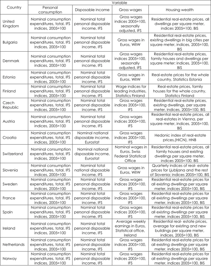
group of post-transition European countries. In order to classify the countries of interest according to the level of national income, the World Bank country classification was employed. Therefore, 11 countries were grouped into developed European countries: Austria, Denmark, France, Finland, Ireland, Netherlands, Norway, Sweden, Switzerland, Spain and United Kingdom. Also, there were 5 countries grouped in post-transition European countries: Bulgaria, Croatia, Czech Republic, Estonia and Slovenia. Detailed description of analysed variables and data sources are given in table A1 in appendix.

In the last fifteen years, the literature on dynamic and co-integrated panels significantly evolved, proposing a number of methods that are designed to handle econometric problems such as the problem of endogeneity and serial correlation of error terms, as well as nuisance parameters, which may occur when assessing the consumption function. Some of these procedures are based on Vector Error Correction Model (VEC), while others are based on individual equations (single-equation models). In this paper, when estimating the effect of housing wealth on consumption, a single equation model and an estimator developed by Pesaran, Shin and Smith (1999) is used. Specifically, this estimator (i.e. Pooled Mean Group, PMG estimator) enables very flexible assumptions in the panel framework, in particular for joint assessment of elasticity of consumption with respect to income and housing wealth, which is achieved by restricting the long-term parameters, and at the same time, short-term parameters, the speed of adjustment and variances are not restricted among countries. Thus, using Auto-regressive distributed lag (ARDL) modelling approach developed by Pesaran, Shin and Smith (1999), PMG estimator can jointly correct for serial correlation between the residuals and the endogeneity of regressors based on the selection of a specific number of lags for both dependent and independent variables.

Data were collected for 16 European countries, and the longest time-span for some countries and variables in the panel is from 1990Q1 to 2012Q1. With regard to the scope of this paper, there are few restrictions concerning the data availability. Specifically, for the implementation of the empirical part of the analysis quarterly data on personal consumption, income and housing wealth were used. Given that in this paper the housing wealth effect on personal consumption is modelled, no distinction between durable and non-durable consumption is made. Namely, according to a research conducted by Mehra (2001), the variable of interest when investigating the wealth effect is the total consumption.

Furthermore, variables for income used in this paper is the total disposable income, since the use of total disposable income instead of just income from work (wages) is proposed in a number of economic theories, such as an extended version of the life cycle theory (see Attanasio et al., 2009).

As a proxy variable for housing wealth the real estate prices are used, since the housing wealth series are not available for some of the developed countries and for most of the post-transition countries in the sample. Real estate prices as a proxy variable for housing wealth are used in a number of research for instance: Aoki, Proudman, Vlieghe (2003), Ludwig, Sløk (2004), Ciarlone (2011), Ahec Šonje, Čeh Časni, Vizek (2012), Čeh Časni (2014), Čeh Časni, Vizek (2014), to name a few.

Data on personal consumption and disposable income are taken from the International Monetary Fund (IFS) database, and data on real estate prices are taken from the Bank for International Settlements (BIS) house price database and national statistics of chosen post-transition countries.

Notwithstanding the unquestionable limitations in the data, the great effort is made in order to make the series of interest as comparable as possible. The property

(5)

34

prices in national currencies are recalculated into base indices (2005 = 100). Finally, all indices are deflated using CPI (consumer price index). In addition, data on personal consumption and disposable income taken from the analytical database of the International Monetary Fund (IFS) offer a certain degree of homogeneity among the countries and therefore are preferred in the analysis, compared to the same data from national statistics.

The variables used in the empirical analysis are expressed in logarithms (i.e. base indices (2005=100) are recalculated to logarithms), so the parameter estimates are interpreted as the elasticity of consumption to changes in the independent variables. Also, variables are seasonally adjusted using the X-12-ARIMA method.

The analysis starts from the equation of personal consumption defined by the following expression: it it i 2 it i 1 i 0 it Y HW C 















,

i



1

,

2

,...,

N

,

t



1

,

2

,...,

T

_i. (1) Namely,

C

_it denotes the logarithm of real private consumption,

Y

_it stands for the logarithm of real disposable income,

HW

_it is logarithm of real housing wealth, and indices i and t indicate the country and time period, respectively. Error term (



_it) denotes the effects of unanticipated tremors in consumption and



₀_i is the constant term.

The equation (1) is resulting from the intertemporal budget constraint, so the coefficients (



₁_iand



₂_i) represent the effects of permanent changes in consumption that have the property of elasticity and are maintainable in the long-run. Furthermore, in the short-run there can be some deviations from long-term relationship given in equation (1) which can happen for various reasons like the adjustment costs, habit persistence or liquidity constraints. Therefore, the typical ARDL consumption pattern as a function of income and wealth includes lags in order to model the response of consumption to changes in income and wealth.

Accordingly, in this paper, econometric specification allows for different functions of consumption by country, simply by means of specifying the lag length for each variable using standard statistical criterion. For simplicity, here is assumed that only the first lag of each variable is relevant in short-term in each country. Consequently, the unrestricted autoregressive distributed lag model, panel ARDL (1,1,1) is given by equation (2): it 1 t , i i 1 t , i i 21 it i 20 1 t , i i 11 it i 10 i it

Y

HW

C



































. (2)

Error term is by the model assumption independently distributed through i and t, but the variance can be heterogeneous across countries. The model assumption of independence through spatial units (cross-section independence) is quite strong and restrictive, since the macroeconomic time series can, in certain cases, reflect a significant degree of correlation among the countries in the panel. Such dependence in the spatial components is the area of panel analyses that is rapidly growing and primarily studies the solution of negative impacts that such dependence causes in existing research instruments. Furthermore, by assumption, the error term in the equation (2) is independent of all other variables. It is also necessary to point out another problem that may arise from the equation (2). Namely, Pesaran, Shin and Smith (1999) showed that the ARDL approach to modelling consumption function is not acceptable in the cases where the variables are not integrated of first order. Thus, reparametrisation of the equality given by expression (2) in order to take into account the possibility of a long-term relationship between the variables obtained by equation (2) in the form of a panel error correction model is given by:

(6)

35



i,t 1 0i 1i it 2i it



11i it 21i it it i it

C

Y

HW

Y

HW

C



















_





, (3)

where Δ is the first difference operator and:

i i 21 i 20 i 2 i i 11 i 10 i 1 i i i 0 i i 1 , 1 , 1 ), 1 (

















           . ₍₄₎

Equation (3) allows for an ARDL (1,0,0) as a exceptional case. Namely, consumption comes in level and with a lag, whereas income and housing wealth only come in level.

Engle and Granger (1987) highlight in their theorem, that there is a connection between the co-integration mechanism and the error-correction mechanism. Thus, equation (3) is the basis for evaluating long-term connection between consumption, income and housing wealth.

Within the defined framework, Pesaran, Shin and Smith (1999) suggest that long-term coefficients in the equation (3) are equal across countries (i.e. long-long-term homogeneity), while the constant, the speed of adjustment, short-term coefficients and error variance may vary by country. In other words, there is a (N-1)* k restrictions on the model given by the expression (3) for each i.

Empirical analysis and results

With the aim of testing the research hypothesis that there is statistically significant and positive long-term relationship between housing wealth and private consumption in the analysed group of European countries, PMG estimator of Pesaran, Shin and Smith (1999) is applied. According to PMG procedure, statistical properties of the variables of interest are tested. In that sense, panel unit root tests with common unit root processes (Levin, Chien-Fu, Chia-Shang, 2002; Breitung, Pesaran, 2005; Hadri, 2000) and with individual unit root processes (Im, Peseran, Shin, 2003; Maddala, Wu, 1999; Choi, 2001) are conducted and summarized in Table 1.

Table 1 Panel unit root tests results

Test _hypothesisNull Alternative _hypothesis

p-values Personal

consumption Disposable income wages Gross Housing wealth Im- Pesaran-Shin All panels contain unit roots Some panels are stationary 0.99 0.99 0.25 1.00 PP-Fischer All panels contain unit roots At least one panel is stationary 0.18 0.00 0.04 0.99 ADF-Fischer All panels contain unit roots At least one panel is stationary 0.74 0.36 0.25 0.84 Levin-Lin-Chu All panels contain unit roots All panels are stationary 0.98 0.99 0.98 0.49

Breitung All panels contain unit roots All panels are stationary 0.99 1.00 1.00 1.00 Hadri All panels are stationary Some panels contain unit roots 0.00 0.00 0.00 0.00

Note: Levin-Lin-Chu, Breitung and Hadri tests require a balanced panel and were therefore applied to a truncated version of the dataset.

(7)

36

In the case of all analysed series, the null hypothesis of a unit root cannot be rejected (and in the case of Hadri test, the null hypothesis of stationarity is strongly rejected). Subsequently, it is confirmed that the series are non-stationary, so panel co-integration tests are carried out.

In the empirical analysis both residual-based (Pedroni, 1999; Kao, 1999), and likelihood-based (Maddala, Wu, 1999) tests for panel co-integration were conducted. In addition, panel co-integration tests based on structural dynamic (Westerlund, 2007), are carried out. The results are presented in table 2.

Table 2 Panel co-integration tests results

Test Null hypothesis Alternative hypothesis Statistics p-value

Westerlund No ECM

All panels contain ECM Gt _Ga 0.085 _0.002 Some panels contain ECM Pt _Pa 0.025 _0.000 Pedroni No cointegration Homogenous cointegration Panel ADF 0.000 Heterogeneous cointegration Group ADF 0.000 Source: calculation of the author.

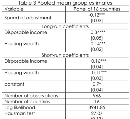
According to table 2, the null hypothesis of no co-integration (or no error correction in case of Westerlund tests) is strongly rejected for all analysed variables. Accordingly, the model given in equation (3) can be estimated and it will offer consistent estimation of the long-run and short-run impact of disposable income and housing wealth on personal consumption. Table 3 summarizes the results of the baseline model.

Table 3 Pooled mean group estimates

Variable Panel of 16 countries

Speed of adjustment -0.12*** [0.03] Long-run coefficients Disposable income 0.34*** [0.05] Housing wealth 0.14*** [0.02] Short-run coefficients Disposable income 0.16*** [0.04] Housing wealth 0.11*** [0.03] constant 0.7* [0.04] Number of observations 966 Number of countries 16 Log likelihood 3941.85 Hausman test 27.07 (0.13)

Note: Estimates are performed using the PMG estimator; the presented short-run coefficients and the speed of adjustment are simple averages of country-specific coefficients; all equations include a constant term; standard errors are given in brackets, p values are given in parenthesis; ***, **, * indicate significance at 1, 5 and 10 percent confidence level, respectively.

(8)

37

The results from Table 3, propose that the error correction mechanism is in position. Thus, the adjustment coefficient has the expected negative sign and is statistically significant at 1% significance level. Therefore, the long-run relationship between personal consumption, disposable income and housing wealth is reached in approximately eight quarters. Furthermore, in the long-run, there is a positive direct housing wealth effect on personal consumption, statistically significant on 1% with the elasticity coefficient of consumption to changes in housing wealth of 0.14. This confirms the research hypothesis of the paper of statistically significant and positive long-term relationship between housing wealth and private consumption in the analysed countries. Also, the housing wealth effect is present in the short-run, with somewhat smaller, but statistically significant coefficient. Furthermore, according to estimated model, disposable income has a significant impact on personal consumption with a positive elasticity coefficient of 0.34. In the short run, disposable income also has a statistically significant positive influence on personal consumption with somewhat smaller coefficient.

In the lower part of Table 3 a test of long-run homogeneity restriction and test of endogeneity bias, which are both Hausman type tests are presented. Nevertheless, homogeneity of long-run coefficients conditional by PMG estimating procedure cannot be assumed in advance. Therefore, two estimators Mean Group (MG) and PMG were compared. In the case when long-run homogeneity restriction is true, PMG gives more efficient estimates compared to MG, but if the true model is heterogeneous, than PMG estimates would be inconsistent. The test result suggests that the null hypothesis of long-run homogeneity restriction cannot be rejected, so the PMG estimator is appropriate in this case.

Conclusions

Given the fact that housing wealth is an important component of total household wealth and it represents the key link between households and the macro economy, in this paper the long-run as well as the short-run link among private consumption, housing wealth, and income was examined. In the empirical analysis of direct housing wealth effect, the pooled mean group estimator for dynamic panel data on the sample of 16 selected European countries was used. The research hypothesis of statistically significant and positive long-term relationship between housing wealth and private consumption in the analysed countries was confirmed. According to the estimated model, the long-run and the short-run housing wealth effect in analysed countries does exist. Furthermore, consumption adjusts to its long-term equilibrium with lags and there is a significant short-term adjustment of endogenous variables (real disposable income and housing wealth) to their long-term relationship with consumption.

In further research, the sample of countries could be enlarged and, also, the different methodology might be used in order to see which variable adjusts the best to the shocks in the real estate prices.

References

1. Ahec Šonje A, Čeh Časni A., Vizek M. (2012). Does housing wealth affect private consumption in European post transition countries? Evidence from linear and threshold models. Post-communist Economies, Vol. 24, No. 1, pp. 73-85.

2. Aoki, K., Proudman, J., Vlieghe, G. (2003). House prices, consumption, and monetary policy: a financial accelerator approach. Bank of England Working Paper Series, No. 169, pp. 1-38.

(9)

38

3. Attanasio, O., Blow, L., Hamilton, R., Leicester, A. (2009). Booms and busts: consumption, house prices and expectations. Economica, Vol. 76, No. 301, pp. 20-50.

4. Babeau, A., Sbano, T. (2002). Household wealth in the national accounts of Europe, the United States and Japan. OECD Statistics Working Papers, No. 2003/02, pp. 1-39.

5. Breitung, J., Pesaran, M. H. (2005). Unit rots and cointegration in panels. In L. Matyas and P. Sevestre (eds.) The Econometrics of Panel data: Fundamentals and recent developments in theory and practice, Springer, pp. 279-322.

6. Bucks, B., Pence, K. (2005). Measuring Housing Wealth, Federal Reserve Board of

Governors, Preliminary draft, January 2005.

7. Choi, I. (2001). Unit root tests for panel data. Journal of International Money and Finance, Vol. 20, No. 2, pp. 249-272.

8. Ciarlone, A. (2011). Housing wealth effect in emerging economies. Emerging Markets

Review, Vol. 12, No. 4, pp. 399-417.

9. Čeh Časni, A. (2014). Housing Wealth Effect on Personal Consumption: Empirical Evidence from European Post-Transition Economies. Czech Journal of Economics and Finance, Vol. 64, No. 5, pp. 392-406.

10.Čeh Časni, A., Vizek, M. (2014). Interactions between Real Estate and Equity markets: an Investigation of Linkages in Developed and Emerging Countries. Czech Journal of

Economics and Finance, Vol. 64, No. 2, pp. 100-119.

11.ECB (2009). Housing Wealth and Private Consumption in the Euro Area. Available at https://www.ecb.europa.eu/pub/pdf/other/mb200901_pp59-71en.pdf [13 December 2016].

12.Engle, R. F., Granger, C. W. J. (1987). Co-Integration and Error Correction: Representation, Estimation, and Testing. Econometrica, Vol. 55, No. 2, pp. 251-276.

13.Friedman, M. (1957). A theory of the Consumption function. Princeton University Press, Princeton.

14.Galì, J. (1990). Finite horizons, life-cycle savings and time-series evidence on consumption.

Journal of Monetary Economics, Vol. 26, No. 3, pp. 433-452.

15.Hadri, K. (2000). Testing for stationarity in heterogeneous panel data. Econometrics

Journal, Vol. 3, No. 2, pp. 148-161.

16.Iacoviello, M. (2011). Housing wealth and consumption, Bord of Governors of the Federal

Reserve System. Available at

https://www.federalreserve.gov/pubs/ifdp/2011/1027/ifdp1027.pdf [13 December 2016]. 17.IFC Bulletin (2009). Measuring financial innovation and its impact. Available at

http://www.bis.org/ifc/publ/ifcb31.pdf [13 December 2016].

18.Im, K. S., Pesaran, M., Shin, Y. (2003). Testing for unit roots in heterogeneous panels. Journal

of Econometrics, Vol. 115, No. 1, pp. 53-74.

19.Kao, C. (1999). Spurious regression and residual-based tests for cointegration in panel data. Journal of Econometrics, Vol. 90, No. 1, pp. 1-44.

20.Labhard, V., Sterne, G., Young, C. (2005). Wealth and consumption: an assessment of the international evidence, Bank of England Working Paper Series, No. 275, pp. 1-51.

21.Levin A., Chien-Fu, L., Chia-Shang, J. C. (2002). Unit root tests in panel data: asymptotic and fnite-sample properties. Journal of Econometrics, Vol. 108, No. 1, pp. 1-24.

22.Ludwig, A., Sløk, T. (2004). The Relationship between Stock Prices, House Prices and Consumption in OECD Countries. The B. E. Journal of Macroeconomics, Vol. 4, No. 1, pp. 1-28.

23.Maddala, G. S., Wu, S. (1999). A comparative study of unit root tests with panel data and a new simple test. Oxford Bulletin of Economics and statistics, Vol. 61, No. 51, pp. 631-652. 24.Mehra, Y. P. (2001). The wealth effect in empirical life-cycle aggregate consumption

equations. Federal Reserve Bank of Richmond Economic Quarterly, Vol. 87, No. 2, pp. 45-68.

25.Paiella, M. (2009). The Stock Market, Housing and Consumer Spending: A Survey of the Evidence on Wealth Effects. Journal of Economic Surveys, Vol. 23, No. 5, pp. 947-973. 26.Pedroni, P. (1999). Critical values for cointegration tests in heterogeneous panels with

(10)

39

27.Pesaran, H., Shin, Y., Smith, R. P. (1999). Pooled Mean Group Estimation of Dynamic Heterogeneous Panels. Journal of the American Statistical Association, Vol. 94, No. 446, pp. 621-634.

28.Westerlund, J. (2007). Testing for error correction in panel data. Oxford Bulletin of

Economics and Statistic, Vol. 69, No. 6, pp. 709-748.

About the author

Anita Čeh Časni is an Assistant Professor at Department of Statistics, Faculty of Economics

and Business, University of Zagreb. Her fields of interest are statistics, econometric modelling of macroeconomic data, panel data linear analysis and housing wealth. She has taken part in several scientific projects and published more than 40 research papers in international scientific journals. She can be contacted at [email protected]

(11)

40

Appendix

Table A1 Data description and sources

Country Personal Variable

consumption Disposable income Gross wages Housing wealth

United Kingdom

Nominal consumption expenditures, total, IFS

indices, 2005=100 Nominal total personal disposable income, IFS Gross wages indices 2005=100, seasonally adjusted, IFS

Residential real-estate prices, all dwellings per square meter,

indices 2005=100, BIS Bulgaria expenditures, total, IFS Nominal consumption

indices, 2005=100 Nominal total personal disposable income, IFS Gross wages in Euros, WIIW

Residential real-estate prices, existing dwellings in big cities per square meter, indices, 2005=100,

BIS Denmark expenditures, total, IFS Nominal consumption

indices, 2005=100 Nominal total personal disposable income, IFS Gross wages indices 2005=100, seasonally adjusted, IFS

Residential real-estate prices, family houses and dwellings per square meter; indices, 2005=100,

BIS Estonia expenditures, total, IFS Nominal consumption

indices, 2005=100

Nominal total personal disposable

income, IFS

Gross wages in

Euros, WIIW Real-estate prices for the whole country, Statistics Estonia Finland expenditures, total, IFS Nominal consumption

indices, 2005=100

Nominal total personal disposable

income, IFS

Wage indices for leading industries, Statistics Finland

Real-estate prices, family houses for the whole country,

Statistics Finland Czech

Republic

Nominal consumption expenditures, total, IFS indices, 2005=100 Nominal total personal disposable income, IFS Gross wages indices 2005=100, IFS

Residential real-estate prices, existing dwellings, per square

meter, indices, 2005=100, BIS Austria expenditures, total, IFS Nominal consumption

indices, 2005=100 Nominal total personal disposable income, IFS Gross wages indices 2005=100, IFS

Residential real-estate prices, all real-estates in Vienna, per square meter, indices, 2005=100,

BIS Croatia expenditures, total, IFS Nominal consumption

indices, 2005=100 Nominal national disposable income, Eurostat Gross wages indices 2005=100, IFS

Hedonic index of real-estate prices,(HICN), HNB Switzerland expenditures, total, IFS Nominal consumption

indices, 2005=100 Nominal national disposable income, Eurostat Nominal wages in Euros, Swiss Federal Statistical Office

Residential real-estate prices, all family houses and existing dwellings per square meter,

indices 2005=100, BIS Slovenia expenditures, total, IFS Nominal consumption

indices, 2005=100 Nominal total national disposable income, IFS Gross wages in Euros, WIIW

Quarterly indices of real- estate prices for Ljubljana and the rest of Slovenia; indices 2005=100, BIS Sweden expenditures, total, IFS Nominal consumption

Residential real-estate prices for all existing dwellings per square

meter, indices 2005=100, BIS France expenditures, total, IFS Nominal consumption

meter, indices 2005=100, BIS Spain expenditures, total, IFS Nominal consumption

meter, indices 2005=100, BIS Ireland expenditures, total, IFS Nominal consumption

indices, 2005=100 Nominal total personal disposable income, IFS Average weekly earnings in Euros, Statistical office, Ireland

Residential real- estate prices, average for existing and new

buildings per square meter, indices, 2005=100, BIS Netherlands expenditures, total, IFS Nominal consumption

meter, indices 2005=100, BIS Norway expenditures, total, IFS Nominal consumption