11-1-2007
Identifiability and Estimation of Causal Effects in
Randomized Trials with Noncompliance and
Completely Non-ignorable Missing-Data
Hua Chen
Peking University, [email protected]
Zhi Geng
Peking University, [email protected]
Xiao-Hua Zhou
University of Washington, [email protected]
This working paper is hosted by The Berkeley Electronic Press (bepress) and may not be commercially reproduced without the permission of the copyright holder.
Suggested Citation
Chen, Hua; Geng, Zhi; and Zhou, Xiao-Hua , "Identifiability and Estimation of Causal Effects in Randomized Trials with Noncompliance and Completely Non-ignorable Missing-Data" (November 2007).UW Biostatistics Working Paper Series.Working Paper 317.
1. Introduction
Two common problems in clinical trials are noncompliance and missing outcome data. Noncompliance occurs when some subjects fail to comply with their assigned treatments; missing data occurs when study investigators cannot collect outcome information on some subjects. Ignoring the noncompliance or missing data may result in biased estimates of causal effects. Moreover, the assumed mechanism of missing-data also has an impact on the estimated causal effects. Many methods have been developed for handling either missing data or noncompliance, but researchers have only recently started to develop methods for handling both missing outcome data and noncompliance in the same study (Frangakis and Rubin, 1999; Zhou and Li, 2006; Yau and Little, 2001; O’Malley and Normand, 2005).
Frangakis and Rubin (1999) proposed a moment estimator for the complier average causal effect (CACE) parameter under the binary compliance status and latent ignorable (LI) missing outcome assumption. The LI assumption means the missing data mechanism has no residual dependence with the outcome, given the observed data and latent compliance class. Under the same LI assumption, Zhou and Li (2006) derived maximum likelihood (ML) estimates as well as moment estimates of the CACE when the compliance status is a discrete variable with three categories and when the outcome variable is binary. O’Malley and Normand (2005) gave the moment and ML estimators of the CACE for a continuous outcome variable.
The above mentioned methods may yield biased estimators of the CACE if the missing data mechanism is a different type of the non-ignorable missing mechanism from latent
ignorability. The mechanism of missing outcome Y may depend on missing values of Y. For
example, some subjects may drop out of a study because of a patient’s declining health
condition, which is related to Y given the observed data and latent compliance class. As
in reducing morbidity in high-risk adults (McDonald et al., 1992). This study began in 1978 and lasted for three years. There were about two thousand patients enrolled in the study. Physicians were randomly assigned to the treatment group of the control group at the beginning of the study. The physicians assigned to the treatment group would encourage their eligible patients to get a flu shot. But the patients themselves decided whether or not to take flu shots. One of the main outcomes in the study was the flu-related hospitalization. Some patients’ outcomes were not observed, and the reason for missing outcomes may depend on the missing values. For example, some subjects were missing their outcomes because they had flu but went to different hospitals than the study hospital, and as a result their outcomes were not recorded. Or, some patients were missing their outcomes because the reason for their hospitalizations was unknown. When the missing data mechanism depends on the outcome, we define this situation as completely non-ignorable (CN). The LI missing data mechanism assumed that subjects dropped out because of subjects’ latent compliance statuses.
Analysis of CN missing data is more difficult than analysis of LI data. One major difficulty under the CN missing data mechanism is the issue of parameter identifiability. Here we
say that a parametric model Pθ is identifiable if there is a unique value of the parameter
vector θ that can generate a given observed distribution Fθ, that is if Fθ = Fθ, then
θ = θ. When the missing-data mechanism is non-ignorable, some of parameters may not
be identifiable even if data provide enough degrees of freedom (Little and Rubin, 2004). Several authors have proposed methods for dealing with CN. For example, Brown (1990) developed an estimation method for missing normal outcome variables in longitudinal studies under the CN missing mechanism. Robins and Rotnitzky (2004) discussed the parameter identifiability in randomized trials with non-compliance. Vansteelandt and Goetghebeur (2005) discussed the parameter identifiability in randomized trials with non-compliance and
missing data. However, no methods are available for dealing with the CN missing mechanism and noncompliance in the same study.
In this paper we fill the gap by first studying identifiability of the model parameters under the CN assumption. We show that the parameters are identifiable under two different conditions. The first condition assumes that the missing data mechanism depends only on the missing outcome variable. If this assumption does not hold, the parameters are not identifiable. However, we can show that the parameters are also identifiable if we can find
an observed discrete covariateX before the treatment assignment, which associated withY
in each subpopulation of the compliance and treatment level. Then we derive both moment and ML estimators.
The paper is organized as follows. We describe notation and assumptions in Section 2. In Section 3, we give the theoretical results on identifiability of the parameters. In Section 4, we conduct simulation studies to assess the finite-sample properties of the derived estimators and sensitivity of the proposed estimators to the departure from the assumed conditions. Then we illustrate the application of the proposed methods in a real study. We give some concluding remarks in Section 5. The proofs of theorems are presented in Appendix.
2. Notation and Assumptions
For the sake of notational simplicity, we suppress the index i, which represents the ith
patient. Let Z represent the randomized treatment assignment (1 =new, 0 = control) and
let ξ = P(Z = 1). Let the binary variable D denote which treatment the patient receives
(1 =new treatment received, 0 =control received). Let D(Z) represent which treatment
received if the patient’s physician is assigned to the treatmentZ, andY be a binary outcome
variable. Y = 0 if the patient goes to the hospital due to the flu andY = 1 otherwise. Ris
the binary response indicator ofY, that is, R= 1 ifY is observed andR= 0 ifY is missing. We define Y{Z, D(Z)} or Y(Z) as the potential outcome of the patient if the patient is
assigned the treatmentZ.R(Z) is the potential binary response indicator of a patient if the patient is assigned to the treatmentZ. In our notation, Z, R,D, and Y are observed data of a patient, and D(Z),Y(Z), andR(Z) are potential outcomes of a patient.
Following Imbens and Rubin (1997), we letU be the compliance status of a patient, defined
as follows: U = ⎧ ⎪ ⎪ ⎪ ⎪ ⎪ ⎪ ⎪ ⎪ ⎨ ⎪ ⎪ ⎪ ⎪ ⎪ ⎪ ⎪ ⎪ ⎩ c, if D(0) = 0 and D(1) = 1 n, if D(0) = 0 and D(1) = 0 a, if D(0) = 1 and D(1) = 1 d, if D(0) = 1 and D(1) = 0,
wherec,n,aanddrepresent complier, never-taker, always-taker and defier, respectively. Here
U is an unobserved variable, representing compliance behavioral patterns of the patient. Let
ωu = P(U = u). For simplicity, we also denote ρyzu = P(R = 1|Y = y, Z = z, U = u)
and θyzu = P(Y = y|Z = z, U = u). As in Imbens and Rubin (1997) and Frangakis and
Rubin (1999), in this paper we consider CACE as the parameter of interest, defined as
CACE=E{Y(1)−Y(0)|U =c}.
Since the joint distribution of the potential outcomes Y(z), R(z) and U conditional on
Z =z can be expressed by parametersωu,ρyzu andθyzu, causal effects are identifiable if we
can show these parameters are identifiable. Next, we will give the necessary assumptions to make these parameters identifiable under the CN missing mechanism.
Assumption 1: Stable unit treatment value assumption (SUTVA) (Rubin, 1978; Angrist et al., 1996; Imbens and Rubin, 1997).
SUTVA implies that potential outcomes do not depend on the treatment status of other individuals.
We can express the CACE asCACE =θ11c−θ10c under the randomization assumption.
Assumption 3: Monotonicity: Di(1) ≥ Di(0) for all subjects i, which implies there are
no defiers.
Assumption 4: Exclusion restrictions (Angrist et al., 1996):P{Yi(1)|Ui=n}=P{Yi(0)|Ui=
n}, and P{Yi(1)|Ui =a}=P{Yi(0)|Ui =a}.
The exclusion restriction impliesP(Yi|Zi = 1, Ui =n) =P(Yi|Zi = 0, Ui =n), andP(Yi|Zi=
1, Ui =a) = P(Yi|Zi = 0, Ui =a), that is θ11n =θ10n andθ11a =θ10a. In some studies, such
as double blinding, exclusion restrictions are reasonable.
Assumption 5: Compound exclusion restrictions (Frangakis and Rubin, 1999):P{Yi(1), Ri(1)|Ui=
n}=P{Yi(0), Ri(0)|Ui =n}, and P{Yi(1), Ri(1)|Ui =a}=P{Yi(0), Ri(0)|Ui =a}.
Assumption 5 is stronger than Assumption 4. Besides having the same implications as Assumption 4, Assumption 5 also implies P(Ri|Zi = 1, Ui = n) = P(Ri|Zi = 0, Ui = n)
and P(Ri|Zi = 1, Ui = a) = P(Ri|Zi = 0, Ui = a). Assumption 4 instead of Assumption
5 is required in our Theorems 1 and 2 where the missing-data mechanism doesn’t depend
on latent compliance status variable U (Assumptions 6 and 7). Assumption 5 instead of
4 is required in Theorems 3 where the missing-data mechanism depends on both missing
outcomes and U (Assumption 8).
3. Identifiability and Estimation
In this section, we discuss additional conditions needed to identify the causal parameters under the CN assumption, and then propose moment and ML estimators of causal effects. Intuition behind how identification of parameters is achieved is related to the idea of in-strumental variables. As we know, if there are no missing outcomes, causal parameters are identifiable under the standard assumptions 1 to 4 of an instrumental variable, as shown
in Angrist, Imbens, and Rubin (1996). When the missing data mechanism depends only on outcomes, under the assumptions 1 to 4, as well as the assumption 6, (U, Z) can be considered as an instrumental variable, and causal parameters are still identifiable. In Section 3.1, we
consider a missing-data mechanism model in which the mechanism of missing outcome Y
depends only on the outcomeY itself; that is, only the outcomeY has an effect onR. Under
this assumption we provide a sufficient condition on parameter identifiability in Theorem 1. Without any other assumptions on the missing data mechanism, only this model and latent ignorable model can be identified.
When the missing data mechanism depends on more variables, an additional instrumental variable is required to identify parameters. If the missing-data mechanism depends on not
only Y but also the treatment assignment Z, we can still identify the parameters in this
model when we have one additional covariate (X) that can affect the outcome Y but does
not depend on the other variablesDandZ in the study. This model is more general than the
first missing-data model. Here (X, U) is being used as an instrumental variable for finding
the effect of Y on R. In Section 3.2, we present the results under this more general model. In Section 3.3, we extend our identifiability results to an discrete outcome with more than two categories.
3.1 Identifiability without Covariate
We consider a CN mechanism which satisfies the following assumption:
Assumption 6: P{Ri(z)|Yi(z), Di(z), U =u}=P{Ri(z)|Yi(z)}for z= 0 and 1, and
P{Ri(1)|Yi(1) =y}=P{Ri(0)|Yi(0) =y}.
WhenZ is randomized, Assumption 6 implies ρyzu =ρyzu for anyz=z oru=u.
Before studying parameter identifiability, we compared Assumption 6 with the LI as-sumption. The LI assumption requires that potential outcomes and associated potential
nonresponse indicators are independent within each level of the latent compliance covariate (Frangakis and Rubin, 1999), that isP{R(1)|U, Y(1)}=P{R(1)|U}andP{R(0)|U, Y(0)}=
P{R(0)|U}. The LI assumption means patients drop out because of their latent compliance class. Yet Assumption 6 means that patients may drop out because of a worsen disease condition, which is related to the outcome. For example, they may drop out when they feel more terrible after taking the assigned drugs. In our study,Y measures the hospitalization of
a subject and the reason for missing Y of a subject may due only to her/his hospitalization
status. So whether patients drop out of the trial is determined by their outcomes, not by their inherent and invariable nature. These two assumptions are so different that a wrong
assumption will have a serious impact on estimation ofCACEunlessCACEis close to zero.
We will see this point in our simulations.
Next theorem shows that the parameters are all identifiable under Assumption 6. For the case of simplicity, we denote ρy = ρyzu and δyzu = P(Y =y, R = 1|Z =z, U = u). Under
Assumption 6, the vector of parameters is θ= (ξ, ωa, ωn, θ10a, θ11n, θ11c, θ10c, ρ0, ρ1).
Theorem 1: If Y is not independent of Z given U or if Y is not independent of U given Z, then under Assumptions 1-4 and Assumption 6, the vector of parameters, θ, is identifiable.
We give a detailed proof of this theorem in Appendix. It is worthwhile to note that if Y is
independent ofZ given U and is also independent ofU givenZ, we can not identify all the
parameters. However, from θ10a = θ11n = θ11c = θ10c, we can get CACE = θ11c−θ10c = 0,
which means the treatment has no causal effect on the outcome.
After we have shown identifiability of θ, we can derive the moment and ML estimators
of θ. Let Nyrzd be the observed number of patients with Y = y, R = r, Z = z, D = d.
The observed data, Ny1zd (for y, z, d = 0,1) and N+0zd (for z, d = 0,1), can be
ν+0zd, where N+0zd =
yNy0zd denotes an observed frequency with y’s value missing,
νy1zd = P(Y = y, R = 1, Z = z, D = d) and ν+0zd = P(R = 0, Z = z, D = d).
Then the moment estimator of CACE is CACE nocova = δ11cρ−1δ10c. And we can obtain that
CACEnocova has an asymptotically normal distribution using the central limit theorem
and the multivariate delta method. Since moment estimates may be the outside of the parameter space in practice (Zhou and Li, 2006), we propose the EM algorithm to find ML estimates in this article. In Theorem 1 the complete-data likelihood function is given as Lc(θ) = ΠNi=1P(Zi)P(Ui)P(Di|Zi, Ui)P(Yi|Zi, Ui)P(Ri|Yi). In the E step, we take the
expectation of the complete-data, given the observed data and the previous parameter estimateθ=θ(k), that is n(yrzuk+1)=E{nyrzu|observed−data,θ(k)}. In the M step, we can get
the ML estimatesθ(k+1) from the n(yrzuk+1).
3.2 Identifiability with a Covariate
In some clinical trials there are good reasons to believe that the missing data mechanism is also affected by the treatment assignment not just the outcome, because the occurrence of side effects differs between treatment arms. In some clinical trials, a direct effect of the treatment assignment on the missing data mechanism is essentially implied by the study design. For example, when patients in the treatment group experience severe side effects, they are removed from further study. Therefore, the response indicator of the outcome,R, depends
not only on the outcome Y itself but also other variables. The parameter vector θ is not
identifiable under only Assumptions 3, 4, and 6 without further assumptions. In this case, we
can introduce an additional covariateXwhich is observed before the assigned treatment, and
thusZ is independent of (X, U). Suppose thatXassociated withY in each subpopulation of
U =u andZ =z (that is,P(y|x, z, u)=P(y|z, u) for somex and for allu andz) such that the parameter vectorθ becomes to be identifiable. For example, in some clinical trials it may
Here we suppose that x is discrete. Then the following theorem shows that parameters are identifiable. Let αxu = P(X = x, U = u), ρyzux = P(R = 1|Y = y, Z = z, U = u, X = x)
and θyzux = P(Y = y|Z = z, U = u, X = x). To emphasize the dependence of the causal
effect parameter on covariates, we write CACE asCACEcova, which is defined as follows:
CACEcova=
xE{Y(1)−Y(0)|U =c, X =x}P(X=x|U =c) =
x(θ11cx−θ10cx)αxc/ωc.
With availability of this covariate X, we can replace Assumption 6 by the following
assumption.
Assumption 7: For z= 0 and 1,
P{Ri(z)|Yi(z), Di(z), U =u, X =x}=P{Ri(z)|Yi(z)}. (1)
Assumption 7 means that the missing data mechanism depends on both the outcomeY and
the assigned treatmentZ, which is weaker than Assumption 6. To identify parameters under
Assumption 7, we introduce an observed covariateX as an additional instrumental variable
in Theorem 2.
When the treatment assignmentZ is randomized, we have from (1) thatρyzux =ρyzux for
anyu=u orx= x, and thus we can simply denoteρyzux asρyz. The vector of parameters,
θ, is denoted asθ = (ξ, ωa, ωn, αxa, αxn, αxc, θ10ax, θ11nx, θ11cx, θ10cx, ρ00, ρ01, ρ10, ρ11).
Theorem 2: Suppose that X is an observed discrete covariate that depends on Y in each subpopulation of U = u and Z =z. Then under Assumptions 1-4 and Assumption 7, the vector of parameters, θ, is identifiable.
We give a proof of Theorem 2 in the appendix. Under the model in Theorem 2, we can obtain
the estimate ofCACE asCACE cova1=
x(δ11cx/ρ11−δ10cx/ρ10)αxc/ωc.
Note that in Theorems 1 and 2 we only make the exclusion restriction assumption, which is weaker than the compound exclusion restriction assumption made in Frangakis and Rubin (1999). If we also make the stronger compound exclusion assumption, we can further relax
Assumption 7 to allow the missing-data mechanism to depend on both missing outcomes and latent compliance status variable.
Assumption 8: For z= 0 and 1,
P{Ri(z)|Yi(z), Di(z), U =u, X =x} = P{Ri(z)|Yi(z), U =u}. (2)
This assumption assumes that the missing data mechanism depends on Y, Z and U.
When the treatment assignment Z is randomized, using (2) we obtain that ρyzux = ρyzux
for any x=x, and thus we can simply denoteρyzux as ρyzu. Since the compound exclusion
assumption (Assumption 5) holds, we have that ρy0n = ρy1n and ρy0a = ρy1a. Hence, the
vector of parameters,θ, is
θ = (ξ, ωa, ωn, αxa, αxn, αxc, θ10ax, θ11nx, θ11cx, θ10cx, ρ11n, ρ01n, ρ00a, ρ10a, ρ11c, ρ01c, ρ00c, ρ10c). Theorem 3: Suppose thatX is an observed discrete covariate that depends onY in each subpopulation of U =u and Z =z. Then under Assumptions 1-3, 5, and 8, the parameters in θ are identifiable.
The difference between the models in Theorems 2 and 3 is in their missing data mechanisms.
For the model in Theorem 3,Rdepends onY(Z),Z andU, whileRdepends only on Y(Z)
andZ in the model of Theorem 2. For the model of Theorem 3, we can obtain the estimate
of CACE asCACE cova2 =
x(δ11cx/ρ11c−δ10cx/ρ10c)αxc/ωc.
3.3 Extension to multi-level outcomes
In this subsection we generalize Theorems 1, 2, and 3 to a multi-level outcome. Let Y be
a K-level discrete variable, where Y = 0, . . . , K −1, and the covariate X be a J−valued variable, i.e., X ∈ {0,1, . . . , J −1}. Since the proofs of corollaries are similar to theorems, we omit the proofs for the sake of simplicity.
matrix, ⎛ ⎜ ⎜ ⎜ ⎜ ⎜ ⎜ ⎜ ⎜ ⎝ δ01n δ11n . . . δK−1,1n δ00a δ10a . . . δK−1,0a δ01c δ11c . . . δK−1,1c δ00c δ10c . . . δK−1,0c ⎞ ⎟ ⎟ ⎟ ⎟ ⎟ ⎟ ⎟ ⎟ ⎠ ,
is equal to K, then the result of Theorem 1 holds.
Note ifK >4, the model of Theorem 1 cannot be identified without additional assumptions,
because the degree of freedom in the observed data is 4K + 3, which is smaller than the
number of parameters 5K−1.
Corollary 2: Let us define the followingJ ×K matrices:
ΔM ultizu = ⎛ ⎜ ⎜ ⎜ ⎜ ⎜ ⎜ ⎜ ⎜ ⎝ δ0zu0 δ1zu0 . . . δK−1,zu0 δ0zu1 δ1zu1 . . . δK−1,zu1 .. . ... . . . ...
δ0zu,J−1 δ1zu,J−1 . . . δK−1,zu,J−1 ⎞ ⎟ ⎟ ⎟ ⎟ ⎟ ⎟ ⎟ ⎟ ⎠ (3) where u=n, a, c and z= 0,1.
(1) When J ≥K, if the ranks of the two J ×K matrices, ΔM ulti1n and ΔM ulti0a , are equal to
K, then the result of Theorem 2 holds.
(2) When J ≥ K, if the ranks of the four J × K matrices, Δ1M ultin , ΔM ulti1c , ΔM ulti0a and ΔM ulti0c , are all equal to K, then the result of Theorem 3 holds.
4. Simulation Studies and Application
In our simulation studies, we first assessed the relative performance of the moment and ML estimators in finite-sample sizes when the assumptions were correct. We then assessed the sensitivity of the derived moment and ML estimators when some of the assumptions were violated.
In the first simulation study, we generated 1000 samples. Each of which had a sample
size of N = 500 under the model with a covariate as specified in Theorems 2. We computed
moment and ML estimates of parameters for every sample, their means, standard deviations, and actual coverage percentages of 95% confidence intervals. The result is reported in Table 1. We used the bootstrap to estimate the standard deviation. Since the moment and ML estimates are all asymptotically normal distributions, we also computed confidence intervals. We also generated data under the missing-data models, given in Theorems 1 and 3. Since the results were similar to that in Theorem 2, we only reported the results on the missing-data model with a covariate in Theorem 2 for the sake of simplicity. From Table 1, we see that
except for ξ, ωn and ωa, the ML estimates perform better than the moments estimators.
In addition, for half of the samples the moment estimates are not proper (meaning that at least one of the estimates for the sample is outside of the corresponding parameter’s range). Hence we would recommend the ML estimates over the moment estimates.
[Table 1 about here.]
Next we conducted a sensitivity analysis of the proposed estimators between the LI as-sumption and CN asas-sumption. We assumed that the true model satisfied the CN asas-sumption
described in Theorem 1, but we estimated the CACE under the wrong LI assumption.
Thus the trueCACEtrue is θ11c−θ10c and the estimated CACEestimated is θ11cρ1θ+(111c−ρ1θ11c)ρ0 − θ10cρ1
θ10cρ1+(1−θ10c)ρ0. Letbias=|CACEestimated−CACEtrue|. We maximized biasover all values
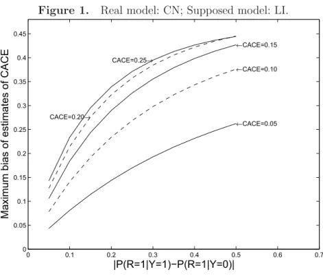
from 0.0 to 1.0 by step 0.01 ofθ11c,θ10c,ρ1andρ0. The result was reported in Figure 1. Each
curve in Figure 1 represents a fixedCACEvalue, which was set to be 0.05, 0.1, 0.15, 0.2, and 0.25, respectively. For each of the five trueCACEtrue values, we plotted a curve to represent
the relationship between the maximum bias of CACE estimates and a real parameter
|P(R= 1|Y = 1)−P(R= 1|Y = 0)|in Figure 1. Here,|P(R= 1|Y = 1)−P(R= 1|Y = 0)| can be interpreted as a measure for the departure of the assumed LI model from the true CN
model. The larger|P(R= 1|Y = 1)−P(R= 1|Y = 0)|is, the further away the assumed LI model is from the true CN model. From Figure 1, we see that the further away the assumed LI model is from the true CN mode, the bigger the bias of the CACE estimates obtained
under the wrong LI model is. From Figure 1, we can also see that the bias of estimated
CACE depends on the value of the true CACE. In general, the larger the true CACE is,
the bigger the bias of the estimated CACE is. As the true CACE decreases, the bias of
the estimated CACE also decreases, and as the CACE value tends to zero, the difference
between the estimates of the CACE under the CN and LI models also tends to zero. [Figure 1 about here.]
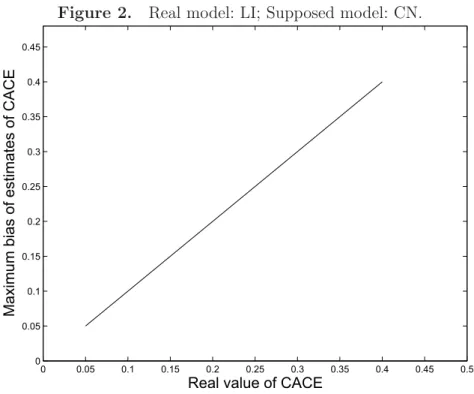
[Figure 2 about here.]
In Figure 2, we assumed that the true missing-data mechanism model was the LI model, but we used a wrong CN model to estimate the CACE. Thus the trueCACEtrueisθ11c−θ10c and
the estimated CACEestimated is (1−
θ11n)γ1n−(1−θ10a)γ0a
γ1nγ0a(θ10a−θ11n) (θ11cγ1c−θ10cγ0c), where γzu = P(R=
1|Z = z, U = u). The bias is still denoted as bias = |CACEestimated − CACEtrue|. We
maximizedbias over all values from 0.0 to 1.0 by step 0.01 of θ11c,θ10c,θ11n,θ10a,ρ1n,ρ0a,
ρ1c and ρ0c. We also found that the maximum bias of the estimated CACE was increasing
as the value of the trueCACE was increasing. Thus, the estimate of CACE is sensitive to
the model of the missing data mechanism. The estimate of theCACE obtained from the LI
model is biased if the true missing-data mechanism is a CN model, and vice versa. On the
other hand, if the value ofCACE tends to zero, the maximum bias tends to zero regardless
whether the true missing-data mechanism model is the CN model or the LI model. Here
the estimate of CACE under the assumption LI is given by Zhou and Li (2006), and the
estimate of CACE under the assumption CN is given by Theorem 1 in this paper.
We also compared our method with the method in which subjects with missing data
of Theorem 1. In Table 2, we reported means and standard errors of estimates of CACE, derived using our method and the method by discarding subjects with missing data. We fix
ρ0= 0.1 and change ρ1 from 0.2 to 0.9 and other parameters are fixed asξ= 0.5,ωn = 0.2,
ωa = 0.3, θ10a = 0.6, θ11n = 0.3, θ11c = 0.8 and θ10c = 0.2. From Table 2, we can see that
the bias of CACE estimates obtained by discarding subjects with missing data increases as
|ρ1−ρ0| is increasing; whereas the estimates obtained by our method are very close to the true CACE regardless of the value of|ρ1−ρ0|.
[Table 2 about here.] [Table 3 about here.]
Now we apply our method to flu shot data, Zhou and Li (2006). We assume the CN
missing-data mechanism satisfying Assumption 6. The observed missing-data are N1100 = 49, N0100 = 573,
N1101 = 16, N0101 = 143, N1110 = 47, N0110 = 499, N1111 = 20, N0111 = 256, N+000 = 492,
N+001 = 17, N+010 = 497, N+011 = 9. We report the results in Table 3. Since the moment
estimates are not proper, we only summarize the ML method. From the table, ρ0 = 1 and
the variance is equal to zero. This result means that all patients who were in hospital must be observed.
The estimated CACE and its 95% confidence interval are -0.1393 and (−0.4808,0.2022)
respectively. For a comparison purpose, we listed the estimated CACE and its 95% confidence interval from Zhou and Li (2006) under the LN assumption. Under latent ignorability, the estimated CACE is -0.009, and its associated 95% confidence interval of CACE is (-0.211,0.229). Both methods reached the same conclusion that influenza vaccination is not associated with reduced risk of hospitalization for respiratory illness.
There are several limitations to the results of this application. First, we ignore clustering effect in the data that may lead to violation of the SUTVA assumption. Second, since the study is not double blind, the exclusion restrictions assumption may be questionable,
particularly among the always-takers, who are probably at high risk for flu and then may receive other medical actions beside flu shots given by their physicians when their physicians received a reminder about flu shots.
5. Conclusion
In this paper we discussed the problem of non-compliance and non-ignorable missing outcome mechanism. One major problem dealing with a non-ignorable missing data is the issue of parameter identifiability. We gave sufficient conditions for identifying causal effect parameters under the CN missing-data mechanism, which is one type of non-ignorable missing and is different from the existing LI assumption. Under the CN missing-data mechanism, we give a theorem on parameter identification when the missing data mechanism depends only on outcomes. With availability of a certain type of covariates, we can relax the missing data mechanism assumption — Assumption 6 — to allow the missing-data mechanism to depend
on not only the missing outcome variable but also the treatment assignment Z and the
latent compliance status variable U. From the simulation results, the estimate of CACE is
sensitive to the missing data mechanism assumption. So we should pay attention to choose the missing data mechanism in practice. It is still an open problem that how to test a non-ignorable missing data mechanism. However, we can obtain from the simulations that the CACE estimates is not sensitive to the missing data mechanism assumption as the true CACE value tends to zero. Some assumptions in our theorems are (partly) testable from the observed data, such as X is not associated with (D, Z).
Acknowledgements
We would like to thank referees for their valuable comments and suggestions that greatly improved the presentation and structure of this paper. This work was supported in part by
NIH/NHLBI grant R01HL62567, NSFC, NBRP 2003CB715900 and IAD-06-088. It does not necessarily represent the views of VA HSR&D Service.
References
Angrist, J. D., Imbens, G.W. and Rubin, D. B. (1996). Identification of causal effects using instrumental variables (with Discussion).Journal of the American Statistical Association
91, 444-472.
Brown, C. H. (1990). Protecting Against Nonrandomly Missing Data in Longitudinal Studies.
Biometrics 46,143-155.
Frangakis, C. E. and Rubin, D. B. (1999). Addressing complications of intention-to-treat analysis in the combined presence of all-or-none treatment-noncompliance and
subse-quent missing outcomes. Biometrika86, 365-379.
Imbenss, G. W. and Rubin, D. B. (1997). Bayesian inference for causal efects in randomized
experiments with noncompliance. The Annals of Statistics25, 305-327.
Little, R. J. A. and Rubin, D. B. (2004). Statistical Analysis with Missing Data Second
Edition. John Wiley & Sons; New York, NY.
McDonald, C.J., Hui, S. L., and Tierney, W. M. (1992). Effects of computer reminders for
influenza vaccination on morbidity during influenza epidemics.M. D. Computing9,
304-312.
O’Malley, A. J. and Normand, S-L. T. (2005). Likelihood Methods for Treatment
Noncom-pliance and Subsequent Nonresponse in randomized Trials.Biometrics 61, 325-334.
Robins, J. and Rotnitzky, A. (2004). Estimation of treatment effects in randomized trials with
non-compliance and a dichotomous outcome using structural mean models. Biometrika
91, 763-783.
Vansteelandt, S. and Goetghebeur, E. (2005). Sense and sensitivity when correcting for observed exposures in randomised clinical trials. Statistics in Medicine24, 191-210.
Yau, L. H. Y. and Little, R. J. (2001). Inference for the complier-average causal effect from longitudinal data subject to noncompliance and missing data, with application to a job
training assessment for the unemployed.Journal of the American Statistical Association
96, 1232-1244.
Zhou, X.H. and Li,S.M. (2006). ITT Analysis of Randomized Encouragement Design Studies
with Missing-Data. Statistics in Medicine25, 2737-2761.
Appendix
Proof of Theorem 1:
Identifiability of ξ, ωa andωn is immediate from randomization of Z and the monotonicity
assumption, that is, ξ = P(Z = 1), ωa = P(U = a) = P(D = 1|Z = 0) and ωn = P(U =
n) = P(D = 0|Z = 1). We next show that δyzu are the functions of the distributions of
observed variables. Under the Assumption 3, we obtain that δy1n = P(Y = y, R = 1|Z =
1, U =n) = P(Y=Py,R(Z=1=1,D,Z=1=0),D=0) and that δy0a = P(Y=Py,R(Z=0=1,D,Z=0=1),D=1).
For δy1c, we have δy1c = P(Y=Py,R(Z=1=1,U,Z==1c),U=c) = P(Y=y,R=1P(,ZZ=1=1,D,D=1)=1)−−PP((YD=1=y,R,Z=1=1,D,U==1a),Z=1,U=a).
Under the monotonicity and randomization assumptions, P(D = 1, Z = 1, U = a) in the
denominator can be rewritten asP(Z = 1)P(D= 1, U =a|Z = 1) =P(Z = 1)P(U =a|Z = 1) = P(Z = 1)P(U = a|Z = 0) = P(Z = 1)P(D = 1, U = a|Z = 0) = P(Z = 1)P(D = 1|Z = 0). On the other hand, from the numerator we have thatP(Y =y, R= 1, D= 1, Z= 1, U =a) = P(R= 1|Y = y, D = 1, Z = 1, U = a)P(Y =y|D = 1, Z = 1, U = a)P(D = 1, Z = 1, U =a), where P(R= 1|Y =y, D= 1, Z = 1, U =a) =P(R= 1|Y =y) =P(R= 1|Y =y, D = 1, Z = 0, U =a) because of Assumption 6, P(Y =y|D= 1, Z = 1, U =a) =
P(Y = y|D = 1, Z = 0, U = a) due to the exclusion restriction andP(D = 1, Z = 1, U =
a) = P(D = 1, U = a|Z = 0)P(Z = 1) by the forward proof. So P(Y = y, R = 1, D =
a)P(D = 1, U = a|Z = 0)P(Z = 1) = P(Y = y, R = 1, D = 1, U = a|Z = 0)P(Z = 1). Hence, we obtain thatδy1c=
P(Y=y,R=1,Z=1,D=1)−P(Y=y,R=1,D=1|Z=0)P(Z=1) P(Z=1,D=1)−P(D=1|Z=0)P(Z=1) .
Similarly, we can show thatδy0c= P(Y=y,R=1P(,ZZ=0=0,D,D=0)=0)−−PP((DY==0y,R|Z=1)=1,DP(=0Z=0)|Z=1)P(Z=0). Hence, we
have shown that δyzu’s are identifiable.
Next we will show that ρy’s are identifiable. Let us define the matrixΔ1 as follows:
Δ1 = ⎛ ⎜ ⎝ δ01n δ00a δ01c δ00c δ11n δ10a δ11c δ10c ⎞ ⎟ ⎠ T .
Becauseθ0zu+θ1zu= 1 and fromδyzu=ρyθyzu, we obtain the following equations:
Δ1 ⎛ ⎜ ⎝ 1/ρ0 1/ρ1 ⎞ ⎟ ⎠ = 1 1 1 1 T . (A.1)
Below we show thatΔ1 has rank 2. Suppose thatΔ1 does not have full column rank. Then
we have δ01n δ11n = δ00a δ10a = δ01c δ11c = δ00c δ10c, which implies θ01n θ11n = θ00a θ10a = θ01c θ11c = θ00c
θ10c sinceδyzu =ρyθyzu.
Thus we obtain that θ10a = θ11n = θ11c = θ10c, which implies that Y is independent of Z
given U and is also independent of U given Z. This contradicts the condition of Theorem
1. Therefore, we have shown that ρy’s are identifiable. Finally, the parameters θyzu can be
identified from equations: θ10n = θ11n = δ11n/ρ1, θ11a = θ10a = δ10a/ρ1, θ11c = δ11c/ρ1 and
θ10c=δ10c/ρ1.
Proof of Theorem 2:
The joint distribution can be factorized asP(Z, U, D, X, Y, R) =P(R|Z, U, D, X, Y)P(Y|Z, U, D, X)
P(D|Z, U, X)P(U, X|Z)P(Z). SinceZ is randomized, P(U, X|Z) =P(U, X). BecauseD is determined by (Z, U), we obtain that P(D|Z, U, X) = P(D|Z, U) and P(Y|Z, U, D, X) =
P(Y|Z, U, X). From the randomization assumption and Assumption 7, we obtain that
P(R|Z, U, D, X, Y) =P(R|Y, Z). So we can rewrite the joint distribution as
To identify P(U, X), we first note that from independence ofZ and (U, X), the definition of
U, and Assumption 3, we obtain thatP(U =a|X =x) =P(U =a|Z = 0, X =x) =P(D= 1|Z = 0, X =x), P(U =n|X = x) = P(U =n|Z = 1, X = x) = P(D = 0|Z = 1, X = x) and then P(U = c|X = x) = 1− {P(U = n|X = x) +P(U = a|X = x)}. Since P(X) is identifiable, P(U, X) is identifiable; since Z and U determine D, P(D|Z = z, U = u) is known for allz and u.
Below we show thatρ01,ρ11,ρ00,ρ10,θ11nx,θ10ax,θ11cx andθ10cx are identifiable
condition-ally on X=x. Let us define the following matrices:
Δ2zu= ⎛ ⎜ ⎝ δ0zux δ1zux δ0zux δ1zux ⎞ ⎟ ⎠ Since
δyzux = P(R= 1|Y =y, Z =z)P(Y =y|Z =z, U =u, X =x) =ρyzθyzux, (A.2)
using the same idea as in the proof of Theorem 1, we obtain the following equations:
Δ21n ⎛ ⎜ ⎝ 1/ρ01 1/ρ11 ⎞ ⎟ ⎠ = ⎛ ⎜ ⎝ 1 1 ⎞ ⎟ ⎠ (A.3) and Δ20a ⎛ ⎜ ⎝ 1/ρ00 1/ρ10 ⎞ ⎟ ⎠ = ⎛ ⎜ ⎝ 1 1 ⎞ ⎟ ⎠. (A.4)
Under Assumption 3, the elements in the matrices Δ21n and Δ20a can be expressed by the distributions of observed variables, respectively, as follows:
δy1nx = P (Y =y, R= 1, Z = 1, D = 0, X =x) P(Z = 1, D = 0, X =x) (A.5) and δy0ax= P (Y =y, R= 1, Z = 0, D= 1, X =x) P(Z = 0, D= 1, X =x) . (A.6)
Suppose that Δ21n in (A.3) is not full rank for all x = x. Then it is immediate that Y is
Thus there exists at least one pair ofx andx so that the matrixΔ21n is full rank, and then
ρ01andρ11can be solved from (A.3). Similarly, we can show thatρ00 andρ10are identifiable from (A.4).
From (A.2), (A.5) and (A.6), we can identifyθy1nxandθy0ax. Similarly we can identifyθy1cx
andθy0cxfrom the equationsθy1cx = δy1cx ρy1 = P(y,R=1,Z=1,D=1,x)/(ξρy1)−P(y,R=1,Z=0,D=1,x)/{(1−ξ)ρy0} P(Z=1,D=1,x)/ξ−P(D=1,Z=0,x)/(1−ξ) andθy0cx= P(y,R=1,Z=0,D=0,x)/{(1−ξ)ρy0}−P(y,R=1,Z=1,D=0,x)/(ξρy1) P(Z=0,D=0,x)/(1−ξ)−P(D=0,Z=1,x)/ξ . Proof of Theorem 3:
Similar to the proof of Theorem 2, we have P(Z, U, D, X, Y, R) = P(Z)P(U, X)P(D|Z, U)
P(Y|Z, U, X)P(R|Y, Z, U). Hence, we can identify δy1nx andδy0ax from (A.5) and (A.6)
re-spectively. We can also identifyδy1cxandδy0cxbyδy1cx=
P(y,R=1,Z=1,D=1,x)−P(y,R=1,D=1,Z=0,x)ξ/(1−ξ) P(Z=1,D=1,x)−P(D=1,Z=0,x)P(Z=1)/P(Z=0)
andδy0cx=
P(y,R=1,Z=0,D=0,x)−P(y,R=1,D=0,Z=1,x)(1−ξ)/ξ P(Z=0,D=0,x)−P(D=0,Z=1,x)P(Z=0)/P(Z=1) .
Next we show that we can identifyρyzu. We first putδyzux’s into the following matrices:
Δ3zu = ⎛ ⎜ ⎝ δ0zux δ1zux δ0zux δ1zux ⎞ ⎟ ⎠,
for (z, u) = (1, n), (1, c), (0, a) and (0, c). Because R is independent of X given (Y, Z, U), we obtain that δyzux = P(R = 1|Y = y, Z = z, U = u)P(Y = y|Z = z, U = u, X = x) =
ρyzuθyzux. Hence, we can obtain the following equations: Δ3zu ⎛ ⎜ ⎝ 1/ρ0zu 1/ρ1zu ⎞ ⎟ ⎠= ⎛ ⎜ ⎝ 1 1 ⎞ ⎟ ⎠.
Using the same argument as in the proof of Theorem 2, we can show that all fourΔ3zumatrices have full ranks under the assumptions in Theorem 3. Therefore, we can identifyρyzu’s. Finally,
becauseδyzux =P(R= 1|Y =y, Z =z, U =u)P(Y =y|Z =z, U =u, X =x) = ρyzuθyzux,
Figure 1. Real model: CN; Supposed model: LI. 0 0.1 0.2 0.3 0.4 0.5 0.6 0.7 0 0.05 0.1 0.15 0.2 0.25 0.3 0.35 0.4 0.45 |P(R=1|Y=1)−P(R=1|Y=0)|
Maximum bias of estimates of CACE
←CACE=0.05 ←CACE=0.10 ←CACE=0.15
CACE=0.20→
Figure 2. Real model: LI; Supposed model: CN. 0 0.05 0.1 0.15 0.2 0.25 0.3 0.35 0.4 0.45 0.5 0 0.05 0.1 0.15 0.2 0.25 0.3 0.35 0.4 0.45
Real value of CACE
Table 1
Simulation results of comparison between moment method and ML method with covariate in Theorem 2, including mean, standard deviation and actual95%coverage probability. The level of covariate is 2 andN= 500.
Moment Method ML Method
Real Parameters Mean Std Dev 95%Cover Mean Std Dev 95%Cover
ξ= 0.5 0.4998 0.0225 0.950 0.4998 0.0225 0.950 P(U =n|X= 0) = 0.3 0.3003 0.0451 0.949 0.2993 0.0448 0.948 P(U =a|X = 0) = 0.2 0.2020 0.0422 0.954 0.2008 0.0419 0.947 P(U =n|X= 1) = 0.1 0.1007 0.0240 0.949 0.1001 0.0239 0.950 P(U =a|X = 1) = 0.5 0.5009 0.0397 0.949 0.4997 0.0393 0.949 P(X = 0) = 0.4 0.3997 0.0229 0.956 0.3997 0.0229 0.956 θ10a0= 0.6 0.7124 0.3501 1.000 0.6201 0.2387 0.995 θ11n0 = 0.3 0.5013 0.3681 1.000 0.2967 0.1169 0.961 θ11c0 = 0.8 0.6835 0.4362 1.000 0.7673 0.1727 0.953 θ10c0 = 0.2 0.3617 0.3806 0.832 0.2398 0.1981 0.941 θ10a1= 0.5 0.6372 0.3430 1.000 0.5236 0.1690 0.966 θ11n1 = 0.2 0.4067 0.3863 0.804 0.2014 0.1301 0.959 θ11c1 = 0.7 0.6224 0.4610 1.000 0.6429 0.2745 0.936 θ10c1 = 0.1 0.2005 0.2614 0.911 0.1194 0.1052 0.956 ρ00= 0.2 0.2331 0.2756 0.916 0.2111 0.0507 0.950 ρ01= 0.3 0.3357 0.2883 0.912 0.3062 0.0793 0.952 ρ10= 0.6 0.4103 0.2760 0.876 0.6271 0.2145 0.999 ρ11= 0.8 0.3515 0.3154 0.639 0.8288 0.1237 0.997 CACE= 0.6 0.3823 0.6703 0.922 0.5254 0.2928 0.933
Table 2
Sensitivity analysis of CNand the method by ignoring incompletely observed subjects. CovariateXis binary and
N= 3000. The true value ofCACEis 0.6.
CACE CACEignor
Value ofρ1 Mean Std Dev Mean Std Dev
ρ1 = 0.2 0.5923 0.0891 0.5621 0.0867 ρ1 = 0.3 0.5992 0.0795 0.5018 0.0715 ρ1 = 0.4 0.5977 0.0754 0.4474 0.0611 ρ1 = 0.5 0.6001 0.0695 0.3983 0.0547 ρ1 = 0.6 0.5987 0.0663 0.3595 0.0490 ρ1 = 0.7 0.5947 0.0636 0.3239 0.0455 ρ1 = 0.8 0.5965 0.0631 0.2998 0.0410 ρ1 = 0.9 0.6017 0.0545 0.2757 0.0376
Table 3
ML estimates and SE of flu shot data.
Parameters MLE Std Dev(Bootstrap) 95% CI
ξ 0.5065 0.0097 (0.4874,0.5255) ωn 0.7839 0.0108 (0.7627,0.8051) ωa 0.1348 0.0091 (0.1170,0.1525) θ10a 0.1757 0.0234 (0.1300,0.2215) θ11n 0.5216 0.0143 (0.4936,0.5495) θ11c 1.379e-016 0.0268 (0.0000,0.0526) θ10c 0.1393 0.1722 (0.0000,0.4768) ρ0 1.0000 0.0000 (1.0000,1.0000) ρ1 0.1151 0.0095 (0.0965,0.1337) CACE -0.1393 0.1743 (−0.4808,0.2022)