New Developments in Planning Accelerated Life Tests

(1)

2009

New Developments in Planning Accelerated Life

Tests

Haiming Ma

Iowa State University

Follow this and additional works at:https://lib.dr.iastate.edu/etd

Part of theStatistics and Probability Commons

This Dissertation is brought to you for free and open access by the Iowa State University Capstones, Theses and Dissertations at Iowa State University Digital Repository. It has been accepted for inclusion in Graduate Theses and Dissertations by an authorized administrator of Iowa State University Digital Repository. For more information, please [email protected].

Recommended Citation

Ma, Haiming, "New Developments in Planning Accelerated Life Tests" (2009).Graduate Theses and Dissertations. 11938. https://lib.dr.iastate.edu/etd/11938

(2)

By

Haiming Ma

A dissertation submitted to the graduate faculty

in partial fulfillment of the requirements for the degree of

DOCTOR OF PHILOSOPHY

Major: Statistics

Program of Study Committee: William Q. Meeker, Jr., Major Professor

Huaiqing Wu Ranjan Maitra

Peng Liu Xiaoli Tan

Iowa State University

Ames, Iowa

2009

(3)

LIST OF FIGURES

FIGURE 2.1:SCALED OPTIMUM VARIANCE AS AFUNCTION OF σ FOR THE WEIBULL ... 17

FIGURE 2.2:SCALED OPTIMUM VARIANCE AS AFUNCTION OF σ FOR THE LOGNORMAL ... 18

FIGURE 2.3:THE OPTIMUM TIME FRACTION OF THE FIRST STEP AND THE LOWER STRESS .... 21

FIGURE 2.4:THE RATIO Avar(y ) Avarˆp _OPT ON ALOG SCALE AS AFUNCTION OF σ FOR THE 24 FIGURE 2.5: SCALED OPTIMUM VARIANCE AS AFUNCTION OF σ FOR THE WEIBULL ... 26

FIGURE 2.6:SCALED OPTIMUM VARIANCE AS AFUNCTION OF σ FOR THE LOGNORMAL ... 27

FIGURE 2.7:SIMULATED SCALED VARIANCE AS AFUNCTION OF THE EXPECTED TOTAL ... 29

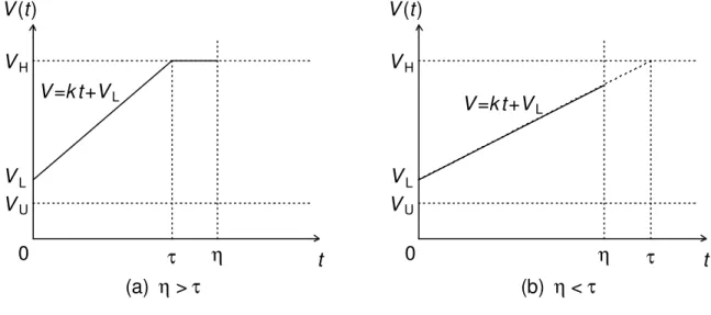
FIGURE 3.1:RAMP-STRESS TEST SCHEMES CONSIDERED IN THIS PAPER. ... 42

FIGURE 3.2:SIMULATED SCALED VARIANCE AS AFUNCTION OF THE EXPECTED TOTAL ... 47

FIGURE 3.3:SCALED OPTIMUM VARIANCE AS AFUNCTION OF σ FOR THE WEIBULL ... 49

FIGURE 4.1:PR(ZFP1)(DOTTED LINE)AND PR(ZFP2)(SOLID LINE)AS AFUNCTION OF N .... 67

FIGURE 4.2:PR(ZFP1)OF OPTIMIZED COMPROMISE TEST PLANS AS AFUNCTION OF π_M ... 68

FIGURE 4.3:THE PLOTS ON THE LEFT SIDE ARE THE SMOOTHED SCALED VARIANCES ... 70

FIGURE 4.4:PR(ZFP1)AS AFUNCTION OF THE UNIT ALLOCATION π_L (LEFT)AND THE ... 72

FIGURE 4.5:SMOOTHED

(

2

)

( ) 0.1 ˆ Var nσ y CONDITIONAL ON NO ZFP2AND

(

n σ2

)

Avar

(

yˆ₀_.₁

)

.. 74

FIGURE 4.6:SMOOTHED

(

n σ2

)

Var

(

yˆ_0.1

)

CONDITIONAL ON NO ZFP2FOR THE 0.1 ... 76

FIGURE 4.7: CONTOUR PLOT SHOWING

(

2

)

(

₀_.₁

)

ˆ Avar y n σ AND ZFP1FOR THE WEIBULL ... 79

FIGURE 4.8: CONTOUR PLOT SHOWING

(

n σ 2

)

Avar

(

yˆ₀_.₁

)

AND ZFP1AT THE CPPV (SOLID ... 81

FIGURE 4.9:SIMULATED

(

2

)

(

₀_.₁

)

ˆ Var y n σ (SMOOTHED SOLID LINES)CONDITIONAL ON NO .... 83

(8)

LIST OF TABLES

(9)

ACKNOWLEDGEMENT

This thesis would not have been possible without the encouragement, support, and patience of my major professor, Dr. William Q. Meeker. I am very grateful to his excellent guidance and kind personal help during my PhD study. I also sincerely thank Dr. Huaiqing Wu, Dr. Ranjan Maitra, Dr. Peng Liu, and Dr. Xiaoli Tan for serving on my thesis committee and for delivering important comments that improved this thesis.

I would like to thank many faculty members in the Department of Statistics for their excellent teachings or help on my research. Among them, I would like to specially

acknowledge Dr. Kenneth Koehler, who encouraged me to complete my PhD program when I began my fulltime job, and also Dr. Dan Nordman, who spent much time helping me do research projects during my PhD study.

I will always remember the people of the staff for their excellent services. Their nice and warm disposition makes me feel as if the department is one big family. Special thanks to Jeanette La Grange, Kathy Shelley, Denise Riker and Norma Elwick for providing help in facilitating my academic tasks.

I have also benefited by my fellow graduate students in this department. In particular, I’m indebted to Hong Yili for his generous help in solving some of course problems. I would like to thank my colleagues and friends in Iowa State University for proving information in many aspects, including job opportunities.

Finally, I would like to thank my wife, Yu He, and my daughters, Xilu Ma and Xili Ma, for their support, encouragement, great patience, and love at all times during my graduate study in Iowa State University.

(10)

ABSTRACT

Accelerated life tests (ALTs) are often used to make timely assessments of the life time distribution of materials and components. The goal of many ALTs is estimation of a quantile of a log-location failure time distribution. Much of the previous work on planning accelerated life tests has focused on deriving test-planning methods under a specific log-location distribution. This thesis presents a new approach for computing approximate large-sample variances of maximum likelihood estimators of a quantile of general log-location distribution with censoring and time-varying stress based on a cumulative exposure model. This thesis also presents a strategy to develop useful test plans using a small number of test units.

We provide an approach to find optimum step-stress accelerated life test plans by using the large-sample approximate variance of the maximum likelihood estimator of a quantile of the failure time distribution at use conditions from a step-stress accelerated life test. In Chapter 2, we show this approach allows for multi-step stress changes and censoring for general log-location-scale distributions. As an application of this approach, the optimum variance is studied as a function of shape parameter for both Weibull and lognormal

distributions. Graphical comparisons among test plans using step-up, step-down, and

constant-stress patterns are also presented. The results show that, depending on the values of the model parameters and quantile of interest, each of the three test plans can be preferable in terms of optimum variance. In Chapter 3, using sample data from a published paper

describing optimum ramp-stress test plans, we show that our approach and the one used in the previous work give the same variance-covariance matrix of the quantile estimator from the two different approaches. Then, as an application of this approach, we extend the

previous work to a new optimum ramp-stress test plan obtained by simultaneously adjusting the ramp rate and the lower start level of stress. We find that the new optimum test plan can

(11)

have smaller variances than that of the optimum ramp-stress test plan previously obtained by adjusting only the ramp rate. We also compare optimum ramp-stress test plans with the more commonly used constant-stress accelerated life test plans.

Previous work on planning accelerated life tests has been based on large-sample approximations to evaluate test plan properties. In Chapter 4, we use more accurate

simulation methods to investigate the properties of accelerated life tests with small sample sizes where large-sample approximations might not be expected to be adequate. These properties include the simulated bias and variance for quantiles of the failure-time

distribution at use conditions. We focus on using these methods to find practical compromise test plans that use three levels of stress. We also study the effects of not having any failures at test conditions and the effect of using incorrect planning values. We note that the large-sample approximate variance is far from adequate when the probability of zero failures at certain test conditions is not negligible. We suggest a strategy to develop useful test plans using a small number of test units while meeting constraints on the estimation precision and on the probability that there will be zero failures at one or more of the test stress levels.

(12)

CHAPTER 1. GENERAL INTRODUCTION

1.1

Introduction

Accelerated life tests (ALT) have been widely used to estimate the lifetime of products in industry. When the lifetime of products at use conditions is much longer than the maximum permitted test time (which is almost always the case), engineers usually increase the levels of stresses (for example, temperature, voltage, humidity, or pressure) to higher than usual levels. They expect that at the higher levels of stress, the products will fail more quickly and that they can estimate the lifetime at use conditions using extrapolations based on an ALT model.

The ALT model usually has two components: a parametric distribution describing the failure-time distribution at fixed level of stress and a relationship between distribution

parameters and levels of stresses. The relationship between life and stress is often proposed by engineers on the basis of physical or chemical theory. Then the engineers can use this relationship to extrapolate the lifetime of products at use level of stress based on parameters estimated from the life-time test at two or more accelerated levels of stress in the interval. If physical or chemical theory is not available, the engineers rely on previous experience to choose a model. If the levels of stress exceed a highest possible level of stress, the linear relationship may no longer hold. Exceeding this critical level of stress should be avoided in practice.

In the ALTs we have considered in this dissertation, we assume that only one accelerating stress is to be considered in designing a test plan and that the failure-time distributions are (log) location-scale distributions. The relationship, after a possible

transformation, is linear between the location parameter of a log location distribution and a transformed level of stress within an interval of stress level bounded by the use level and

(13)

another highest level at which testing will be permitted. We also assume that the scale parameter of the log-location-scale distribution does not depend on the level of stress.

There are several types of the ALT plans that have been proposed in the literature and that have been used in practice. Among them the most commonly used and extensively studied one is the constant-stress test plan. In a constant-stress test plan, the test units are allocated to two or more groups of different levels of stress. Usually, all the test units begin the test simultaneously and the test is run until a common censoring time. Recently, step-stress test plans have also drawn much attention. In a step-step-stress test plan, all the test units are tested at a common level of stress. The level of stress, however, can increase or decrease at points in time. If the change of stress levels is continuous, then we have a progressive-stress accelerated test plan. A progressive-progressive-stress AT plan with a constant rate of change leads to an important special case known as a ramp-stress test plan. In test plans other than

constant-stress test plans, it is necessary to assume a cumulative exposure model that specifies how the probability of failure is affected as the level of stress changes over time. The cumulative exposure theory used in our research has been described in [3].

In designing a constant-stress test plan, engineers need to determine the allocations of test units to different groups and the level of stress for each group. In designing a step-stress or a ramp-stress test plan, engineers need to determine how the level of stress changes over time. In either case, before designing such a test plan, the engineers need information about the underlying distribution, the probability of failure of test units at two levels of stress. Such information, which is known as “planning information” or “planning values” of the

parameters, is typically based on their previous experience with similar products or engineering judgment. The planning values are usually uncertain, which means that engineers usually only provide a range of the planning values that they believe contain the true underlying values.

(14)

The role of a statistician in designing an ALT plan is to help engineers with a specified amount of limited resources to get the most accuracy and precision from their experiment. Because maximum likelihood (ML) estimation is commonly used to analyze ALT data, a useful criterion for planning an ALT test is to minimize the variance of the ML estimator of some quantiles of a log location-scale distribution at the use conditions. This is usually done by comparing the large sample approximate variance of the estimators obtained from by inverting the Fisher information matrix for different test plans. If there were no uncertainty in our planning values, one could use an optimum test plan which, among all possible test plans, has the smallest variance of the estimator. In practice, however, there is always uncertainty in planning information and thus, as an alternative, it has been suggested that one should use a compromise test plan that has good (but not optimum) statistical properties, but that is also is robust to the uncertainty of the planning values.

A number of papers have been published to describe methods of designing optimum and compromise constant-stress, step-stress, and ramp-stress test plans using some well-known log location scale distributions, such as the exponential, Weibull and lognormal distributions. Most of the published work in this area has only aimed at analyzing the properties corresponding to a specific log location distribution and a specific type of test plans used in the papers. We know of no previous work that has, in these general cases, compared the variances of the ML estimators of a quantiles of a log location-scale

distribution among constant-stress, step-stress and ramp-stress with censoring. At the same time, in practical applications, engineers want to know which type of test plans is more appropriate for their specific problem than others types of test plans. The research work presented in Chapters 2 and 3 are motivated by these kinds of questions.

Previous work on designing ALT plans has usually used the large-sample

approximation approach. This approach is, however, questionable for the cases with a small numbers of test units. Yet, engineers are often constrained to use the smallest number of test

(15)

units possible to make some kind of reasonable estimate of life at use conditions. The test plan designs obtained from large sample approximations applied to tests that actually have a small numbers of test units could be misleading. Studies along these lines have not been developed so far. The research work presented in Chapter 4 is motivated by these kinds of questions.

1.2 Overview of Available Literature

There is much literature describing research that has been done on ALT data analyses and on ALT plan designs. For example, Chapter 6 of Nelson [3] reviews constant-stress ALT plans. Chapter 10 of [3] describes step-stress and ramp-stress test plans and how to do data analyses, and gives references to the original sources.Chapters 18-20 of Meeker and Escobar [2] provided basic knowledge, detailed information and practical suggestions on ALT

models, data analysis and test planning for constant-stress ALTs. Nelson [4, 5] provides an extensive bibliography describing much of the previous research work that has been done to study accelerated test plans. Escobar and Meeker [1] reviewed the ALT models that are commonly used in practice.

1.3 Dissertation Organization

This dissertation consists of three papers corresponding to Chapters 2, 3, and 4, respectively. Chapter 2 provides an approach for designing step-stress ALT plans for a general log-location-scale distribution. The approach includes the derivation of a general log likelihood for the associated cumulative exposure model, its derivatives with respect to distribution parameters, and expectations needed to compute the Fisher information matrix. Comparison of the large-sample approximate variance is presented among constant-stress,

(16)

step-up-stress, and step-down-stress test plans under the same planning values for different log location-scale distributions.

Chapter 3 extends the approach of Chapter 2 to a limiting case with a continuously varying level of stress for a general log-location-scale distribution. We found that the values of the variance–covariance matrix from our general algorithm correspond to the value obtained from a different approach (only valid for Weibull distribution) proposed in a previously published paper. We also extend the one-dimensional optimum ramp-stress test plan that has been presented previously in the literature to a better two-dimensional optimum ramp-stress test plan. We also compare the new optimum test plan with the optimum

constant-stress test plans under the same planning values.

Chapter 4 discusses how to choose a constant-stress test plan efficiently to meet a requirement of the precision in estimating lifetime of products when there are stringent constraints on the number of units that can be tested. We focus on practical three-level test plans because they are most commonly used in actual applications. We study the impact that not having any failures at test conditions will have on lifetime estimation. We then suggest and illustrate the use of a strategy combining both the conventional large-sample

approximation approach and the more accurate simulation approach together. This strategy can be used to find a good test plan. In particular, these test plans have the smallest variance of the estimation while holding the probability of not having any failures at test conditions below a critical level and keeping the sample size as small as possible.

Chapter 5 provides overall conclusions based upon the results obtained in Chapters 2, 3 and 4. Two appendices are provided for the details in deriving formulas in Chapters 2 and 3, respectively.

(17)

References

[1] Escobar, L. A. and Meeker, W. Q., “A Review of Accelerated Test Models,”

Statistical Science 21, 552–577 (2006).

[2] Meeker, W. Q. and Escobar L. A., Statistical Methods for Reliability Data, Wiley, New York, 1998.

[3] Nelson, W., Accelerated Testing-Statistical Models, Test Plans and Data Analysis, Wiley, New York, 1990.

[4] Nelson, Wayne, “A Bibliography of Accelerated Test Plans, Part I−Overview,” IEEE Trans. on Reliability, R-54 (2005), 194-197.

[5] Nelson, Wayne, “A Bibliography of Accelerated Test Plans, Part II−References,”

(18)

CHAPTER 2. OPTIMUM STEP-STRESS ACCELERATED

LIFE TEST PLANS FOR LOG-LOCATION-SCALE

DISTRIBUTION

Haiming Ma and W. Q. Meeker Department of Statistics

Iowa State University Ames, IA 50011

Abstract

This paper presents new tools and methods for finding optimum step-stress accelerated life test plans. First, we present an approach to calculate the large-sample approximate variance of the maximum likelihood estimator of a quantile of the failure time distribution at use conditions from a step-stress accelerated life test. The approach allows for multi-step stress changes and censoring for general log-location-scale distributions based on a cumulative exposure model. As an application of this approach, the optimum variance is studied as a function of shape parameter for both Weibull and lognormal distributions. Graphical comparisons among test plans using step-up, step-down, and constant-stress patterns are also presented. The results show that, depending on the values of the model parameters and quantile of interest, each of the three test plans can be preferable in terms of optimum variance.

Key Words – Cumulative exposure model, Large-sample approximate variance, Maximum likelihood.

(19)

Notation

U

s , s_H pre-specified use stress and highest possible stress

h

s s

s₁ , ₂ ,K , _{test stress levels}

h total number of stress levels in the experiment

ξ standardized stress level

i

τ time of stress change from s_i to s_i₊₁ at each step, i =1,2,K,h−1

t, η failure time and censoring time

σ

µ , location and scale parameters of a location-scale distribution

1 0 ,γ

γ parameters of the log linear regression model

( )

⋅

φ , Φ

( )

⋅ pdf and cdf of a location-scale distribution H

U p

p , probabilities that a unit will fail by time η at use and the highest stress levels, respectively

p

z p quantile of a standard location-scale distribution

( )

ξ

p

p y

y = p quantile of a location-scale distribution at stress level ξ

n total number of test units

2.1 Introduction

2.1.1 Accelerated Testing Background

In accelerated life tests (ALTs), units are tested at higher levels of stress (e.g., temperature, voltage, pressure) to obtain information about reliability in a small amount of

(20)

time. ALTs are commonly used in product test plan processes (e.g., Nelson [10-14], Meeker and Escobar [8] and Escobar and Meeker [4]). Techniques for performing an ALT include constant stress (e.g., Chapter 6 of Nelson [14], Meeker and Hahn [7], Chapter 19 of Meeker and Escobar [8]) and step stress (e.g., Nelson [11], Chapter 10 of Nelson [12]).

In an ALT with constant stress, all the units are allocated into two or more groups to be tested separately at specified stress levels. When possible, the tests are run simultaneously to save time. In a step-stress ALT, units begin at a specified stress level. After a time fraction with respect to the total test length, the stress level is changed to another level. The stress level can be changed more than once before the end of the test. An advantage of step-stress ALTs is that increasing the level of stress during the test will generally result in failures happening more quickly. Another advantage of step-stress ALTs is that only one temperature-control chamber is needed. In a step-stress test all units are at a common temperature which changes at the step. In constant-stress ALTs there are usually separate chambers for each level of temperature.

Different choices of test-stress levels and unit allocations (for constant stress) or time fraction (for step stress) can result in different estimation precision of a quantity of interest such as a quantile of the life distribution at use conditions. Our goal is to compare test plans in terms of the optimum (i.e., the smallest) variance of maximum likelihood (ML) estimates and to provide insight and tools that can be used to find a practical, statistically efficient accelerated test plan.

2.1.2 Previous work in planning accelerated tests

A number of research papers have developed methods for optimum and robust ALT test plans by suitably choosing test length, levels of accelerating variables and allocation of test units. It is often assumed that the purpose of an ALT is to estimate a quantile of the failure distribution at use conditions. The criterion for choosing an ALT plan is often to find

(21)

a plan that gives minimum variance of the ML estimator of a particular quantile. In this section we describe related previous work on planning step-stress experiments. Within the framework of Nelson’s cumulative exposure model [12], Miller and Nelson [9] first

presented theory for optimum test plans for a single-step stress test with complete failure data (i.e., all units run to failure) from an exponential distribution. Bai, Kim and Lee [2] extended the theory of Miller and Nelson to censoring. Their work was further extended to optimum multi-step step-stress by Khamis and Higgins [5] and Yeo and Tang [16] and to type II censoring under the exponential distribution by Xiong [15].

Optimum multi-step-stress test plans have also been developed using the Weibull and lognormal distributions with censoring. Bai and Kim [3] developed an approach to multi-step stress for the Weibull distribution with the highest stress level at the last step. More recently, Alhadeed and Yang [1] obtained optimum step-stress plans for complete failure data using the lognormal distribution.

Miller and Nelson [9] compared constant and step-stress test plans for the exponential distribution. Their results showed that step-stress tests yielded the same amount of

information as constant-stress tests under the exponential distribution with complete failure data. They optimized their step-stress plan by choosing the time of the step that minimizes the approximate variance of the ML estimator of a quantile of interest in their test plans.

Khamis [6] compared constant stress and step-stress test plans for the Weibull distribution with a known shape parameter and fixed lower stress. His results showed that step-stress test plans may have an advantage over constant-stress test plans when there is heavy censoring for the constant-stress test at lower stress levels.

Although much work has been done to find optimum step-stress ALT plans, the tradeoffs between constant and step-stress testing in terms of variance of ML estimation of quantiles of the failure time distributions has not been clearly evaluated. Within the step-stress test plans, focus has been on the step-up because it is thought to assure failures quickly.

(22)

Step-down test plans also have potential value. The idea is that initial aging of units at high stress could provide more failures at lower levels of stress and thus better information when the test is continued at lower levels of stress. Also, previous research for step-stress ALTs has been for particular distribution like the exponential, Weibull and lognormal distributions. We extend Bai and Kim’s results [3] to provide a more general theory and methods for multiple-step stress ALTs for the log location-scale family of distributions. The optimization is done with respect to both positions of the steps and stress fractions in step-stress,

simultaneously. The different properties among constant, step-up-stress, and step-down-stress test plans are presented graphically with respect to the optimum variance of failure-quantile estimators.

2.1.3 Overview

In section 2.2, we describe three test plans that are used in this paper. In section 2.3, we present the model that we use to minimize the large-sample approximate variance of the ML estimator of a specified quantile of a log location-scale distribution in a general multi-step-stress ALT. Section 2.4 shows the optimum variance for a simple multi-step-stress test as a function of the shape parameter of the Weibull and lognormal distributions for different combinations of the planning values. This section also presents comparisons between simple step-stress and constant-stress test plans. Section 2.5 provides some concerns in practical applications including compromise test plans and an assessment of the effect of incorrectly specifying the planning value forσ . Section 2.6 gives some simulation results to check the adequacy of the large-sample approximate variances. Section 2.7 draws some conclusions and outlines areas for future research in this area.

(23)

2.2 Test Plans

In this paper, we compare the optimum large-sample approximate variances of the ML estimators among three basic test plans. In most ALT models there is an implied

transformation of stress (e.g., log of voltage). We use s to denote this transformed stress. All tests will be between the use stresss_Uand the highest possible stress s_H. Under the three test plans, test units are tested at the pre-specified highest stress levels_H and at another stress level s_L wheres_U ≤s_L <s_H. For convenience, in the following we use the standardized stress ξ =

(

s−sU

) (

/ sH −sU

)

, where 0≤ξ ≤1. Thus ξU =0, ξH =1. The maximum test length is η.

The three test plans compared in this paper are (1) Constant-stress test plan

When only two stress levels are involved, all of the test units are divided into two groups. One group is tested at ξ_H and the other group is tested at ξ_L. Both groups are tested simultaneously from the beginning until the censoring time η. When three stress levels are involved, all of the test units are divided into three groups. One group is tested at ξ_H, another group is tested at ξ_L and the third group is tested at a stress being the middle of ξ_L and ξ_H. Three groups are tested simultaneously from the beginning until the censoring time η. (2) Step-up stress test plan

When only two stress levels are involved, all of the test units begin the test at ξ_L. At timeτ₁

(

τ₁ <η

)

, all of the surviving units are moved to ξ_H and tested until time η. This is called a simple step-up stress test plan. When three stress levels are involved, all of the test units begin the test at ξ_L. At time τ₁

(

τ₁ <η

)

, all of the surviving units are moved to a stress being middle of ξ_L and ξ_H until τ₂

(

τ₁ <τ₂ <η

)

. Then all of the surviving units are moved to ξ_H and tested until time η.

(24)

When only two stress levels are involved, all of the test units begin the test at ξ_H. At timeτ₁

(

τ₁ <η

)

, all the surviving units are moved toξ_L and tested until timeη. This is known as a simple step-down stress test plan. When three stress levels are involved, all of the test units begin the test at ξ_H. At timeτ₁

(

τ₁ <η

)

, all of the surviving units are moved to a stress midway between ξ_L and ξ_H and tested untilτ₂

(

τ₁ <τ₂ <η

)

. Then all of the surviving units are moved to ξ_L and tested until timeη.

When only two stress levels are involved, by changing ξ_L and the allocation of the test units at ξ_L simultaneously for constant-stress test plans or by changing ξ_L and τ₁

simultaneously for step-stress test plans, one can obtain the optimum test plans characterized by the large-sample approximate variance of the ML estimators. When three stress levels are involved, we consider a case with a fixed allocation of the test units (for constant) and fixed time duration τ₂ −τ₁ (for step-stress)at the middle level of stress. Then the optimum test plans can be obtained by changing ξ_L and the allocation of the test units at ξ_L

simultaneously for constant-stress test plans or by changing ξ_L and τ₁ simultaneously for step-stress test plans.

2.3 The Model and Log Likelihood

2.3.1 Model

We assume that at any level of stress the failure time T follows a log location-scale distribution with constant σ and cdf

Pr[T≤t;Τ] = Φ _      − σ µ ) log(t ,

where the location parameter is µ =γ₀ +γ₁ξ . We also assume that Nelson’s [12] cumulative exposure model holds. This model implies that the distribution of remaining life of a test unit depends only on the cumulative exposure it has received no matter how it was exposed. Let

(25)

( )

t

z_i , the standardized log time at stress level i, be defined as zi =

[

log

(

t−δi−1

)

−µ

( )

ξi

]

σ ,

h

i₌2,3,K, _{, and}

[

(

_η _δ

)

_µ

( )

_ξ

]

_σ

η h h

z = log − −1 − , where τi−1 ≤t≤τi and τi is thetime of stress change from s_i to s_i₊₁ with τ₀ =0and h is the total number of stress levels in the experiment.

The time shift induced by the change in stress levels from the beginning of the test to the beginning of step i is

(

)

(i j) e i j j j i i ξ ξ γ

τ

δ

− − = − − − = −

∑

− 1 1 1 1 1 1 .

Note that δ_i₋₁ is positive for a step-up stress test plan and negative for a step-down stress test plan, because γ₁ is typically negative. Under the cumulative exposure model, we havez_i

( )

τ_i =z_i₊₁

( )

τ_i , i₌2,3,K,h_.

The failure probabilities at the highest stress (ξH =1) and the lowest stress (ξU =0)

are:       − − Φ = σ γ γ η) ₀ ₁ log( H p and       − Φ = σ γ η) ₀ log( U

p , respectively. It is easy to express

the failure probability at any value of ξ as a function of p_Uandp_H.

2.3.2 Log likelihood

The likelihood for a single test unit having a log location-scale failure time distribution under a multi-step-stress test is:

L =

(

)

( )

[

]

U ( )t t U i i h i h i z z t 1 1 1 1 1 + Φ −       − Π − = σ δ φ η ,

where U_i

( )

t = 1 if t is within the step of ξ_i and zero otherwise, i=1,2,⋅⋅⋅⋅⋅⋅h. U_h₊₁

( )

t = 1 if

t is larger than η and zero otherwise. The log likelihood for a single test unit is

(

)

[

]

{

log( ) log log ( )

}

( )log

[

1 ( )

]

) ( ₁ 1 1 φ η δ σ t z U t z t U l _h h i i i i − − − + + −Φ = + = −

∑

. (1)

(26)

The first and the second partial derivatives of (1) with respect to the model

parameters are given in the appendix. The total log likelihood is obtained by summing (1) over all test units. The ML estimators γˆ₀, γˆ₁ and σˆ are those values that maximize the total log likelihood.

2.3.3 The large-sample approximate variance

In models that meet standard regularity conditions (including the log location scale distributions used in this paper), the Fisher information matrix can be used to quantify the expected information that an experiment will provide on a set of parameters. Also, the large-sample approximate variance-covariance matrix of the ML estimators is the inverse of the Fisher information matrix. Details are presented in the appendix.

Our goal is to minimize the large-sample approximate variance of the ML estimator of the p quantile of the log failure time distribution at the use stress. The ML estimator of the

p quantile at stress level ξ can be expressed as

σ ξ γ γˆ ˆ ˆ ˆ_p ₀ ₁ z_p y = + + .

The large-sample approximate variance of yˆ_p is Avar(yˆp)=

(

1,ξ,zp

)

Σγˆ₀,γˆ₁,σˆ

(

1,ξ,zp

)

T,

whereAvar is used to denote the large sample approximate variance of a scalar quantity,

σ γ

γˆ₀,ˆ₁,ˆ

Σ is the large-sample approximate variance-covariance matrix given in the appendix, and the superscript T indicates vector transpose. Our objective is to minimize Avar(yˆp) at

. 0

=

ξ The test plan properties to be optimized are τi and ξi, i=1,2,K,h−1. The

optimization can be done using the function optim() in R. To solve the problem of multiple optima, multiple start values are necessary to achieve the minimum variance in the

(27)

For comparing the relative efficiency of test plans with different samples sizes we can use the scaled large-sample approximate variance defined as

(

_σ2

)

n Avar(yˆp). The large-sample approximate variance-covariance matrix and properties of optimum test plans depend only on the planning values p_H , p_U andσ. This is because given p_H ,p_U, σ and a

censoring time η, one can calculate γ₀ and γ₁, providing a complete specification of the model and the amount of censoring for the test plan. These planning values are usually obtained from previous experience with a similar product or from engineering judgment.

2.4 Comparison of Simple Step-Stress and Constant-Stress Plans

2.4.1 Comparison of approximate variance

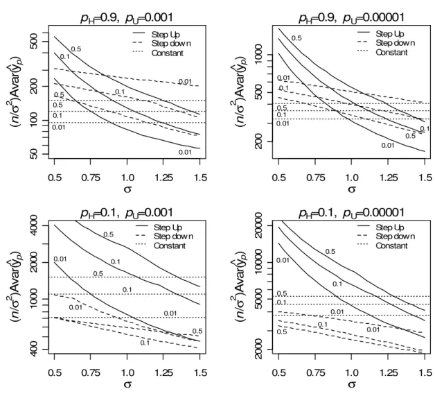
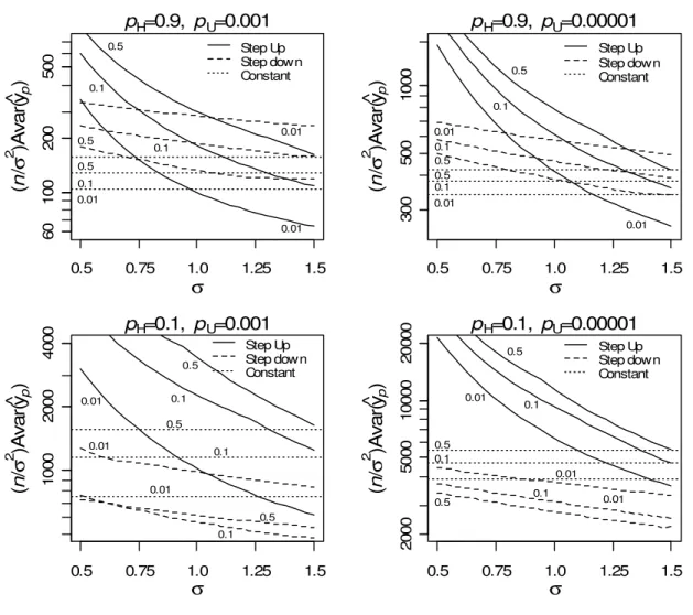
Figures 2.1 and 2.2 show the value of scaled variance

(

_σ2

)

n Avar(yˆp) obtained from optimum ALT plans with two stress levels as a function of σ for three different

quantiles of interest: 0.01, 0.10 and 0.50. These figures also compare constant-stress, step-up-stress, and step-down-stress test plans for different values of p_H and p_U under the Weibull and lognormal distributions, respectively. Some important conclusions from these figures are:

(28)

p_H=0.9, p_U=0.001 Step Up Step down Constant 5 0 1 0 0 2 0 0 5 0 0 0.5 0.75 1.0 1.25 1.5 0.1 0.01 0.5 0.1 0.01 0.5 0.5 0.1 0.01 σ ( n / σ 2 )A v a r( y^p ) p_H=0.9, p_U=0.00001 Step Up Step down Constant 2 0 0 5 0 0 1 0 0 0 0.5 0.75 1.0 1.25 1.5 0.5 0.1 0.01 0.1 0.01 0.5 0.5 0.1 0.01 σ ( n / σ 2 )A v a r( y^p ) p_H=0.1, p_U=0.001 Step Up Step down Constant 4 0 0 1 0 0 0 2 0 0 0 4 0 0 0 0.5 0.75 1.0 1.25 1.5 0.5 0.1 0.01 0.5 0.1 0.01 0.5 0.1 0.01 σ ( n / σ 2 )A v a r( y^p ) p_H=0.1, p_U=0.00001 Step Up Step down Constant 2 0 0 0 5 0 0 0 1 0 0 0 0 2 0 0 0 0 0.5 0.75 1.0 1.25 1.5 0.5 0.1 0.01 0.5 0.1 0.01 0.5 0.1 0.01 σ ( n / σ 2 )A v a r( y^p )

Figure 2.1: Scaled optimum variance as a function of σ for the Weibull distribution at three quantile of

interest for four combinations of planning values under three test plans. The three quantiles of interest

are p = 0.01, 0.1 and 0.5, respectively. The four combinations of planning values are (p_H = 0.9, p_U =

0.001), (p_H = 0.9, p_U = 0.00001), (p_H = 0.1, p_U = 0.001), and (p_H = 0.1, p_U = 0.00001),

respectively. The three test plans investigated are step-up stress, step-down stress and constant stress, respectively.

(29)

p_H=0.9, p_U=0.001 Step-up Step-down Constant 1 0 2 0 5 0 1 0 0 0.5 0.75 1.0 1.25 1.5 0.5 0.01 0.1 0.5 0.1 0.01 0.5 0.1 0.01 σ ( n / σ 2 )A v a r( y^p ) p_H=0.9, p_U=0.00001 Step Up Step down Constant 2 0 5 0 1 0 0 2 0 0 0.5 0.75 1.0 1.25 1.5 0.01 0.5 0.1 0.5 0.1 0.01 0.1 0.5 0.01 σ ( n / σ 2 )A v a r( y^p ) p_H=0.1, p_U=0.001 Step Up Step down Constant 1 0 0 2 0 0 5 0 0 2 0 0 0 0.5 0.75 1.0 1.25 1.5 0.1 0.01 0.5 0.1 0.01 0.5 0.01 0.1 0.5 σ ( n / σ 2 )A v a r( y^p ) p_H=0.1, p_U=0.00001 Step Up Step down Constant 3 0 0 5 0 0 1 0 0 0 2 0 0 0 0.5 0.75 1.0 1.25 1.5 0.5 0.1 0.01 0.5 0.1 0.01 0.01 0.1 0.5 σ ( n / σ 2 )A v a r( y^p )

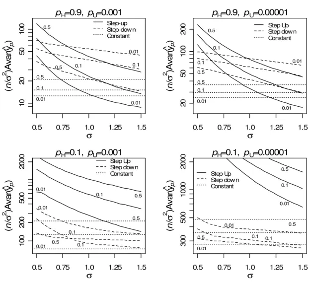
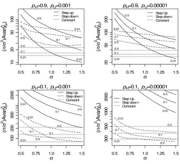
Figure 2.2: Scaled optimum variance as a function of σ for the lognormal distribution at three quantile

of interest for four combinations of planning values under three test plans. The three quantiles of interest

0.001), (p_H = 0.9, p_U = 0.00001), (p_H = 0.1, p_U = 0.001), and (p_H = 0.1, p_U = 0.00001),

respectively. The three test plans investigated are step-up stress, step-down stress and constant stress, respectively.

(30)

a) In the step-up and step-down test plans, the scaled optimum variance usually decreases as σ increases. As it is known from previous work (e.g., Nelson and Kielpinski [12]), the scaled variance for constant-stress plans does not depend on σ. b) Step-up plans are usually poor relative to step-down plans when p_H is small.

Depending on the planning values, step stress plans can have either a smaller or a larger optimum variance than constant stress plans. For plans with small σ and large

H

p , the constant-stress plans are usually better than the step-stress plans.

c) Given the same values of p_H and p_U, the optimum variance of the 0.10 quantile ML estimator is usually larger than that of the 0.01 quantile and smaller than that of the 0.50 quantile in a step-up plan. Constant-stress plans have the same ordering as that of step-up stress plans. Interestingly, the curves for a step-down plan have the reverse order. However, this reverse order can change when p_H and p_U approach each other as shown in the SW corners of Figures 2.1 and 2.2.

d) Comparing test plans with the same values of p_H and p_U, the test plans under the lognormal distribution have a smaller optimum variance than those for the

corresponding Weibull distributions. This is because a lognormal distribution has a lighter lower tail than that of the corresponding Weibull distributions with the same first-two moments. Thus, with the same amount of change in the lower tail of the distribution, the corresponding change the log quantile y_pof the lognormal distribution is smaller than that of the Weibull distribution. Note also that the relationship between the shape parameter and the variance of ML estimators of quantiles of a Weibull distribution is different from that of a lognormal distribution (see, e.g., [8], page 83). This fact needs to be considered when comparing the optimum variances between the two distributions with the same planning values p_H

(31)

2.4.2 Comparison of Test Plan Parameters

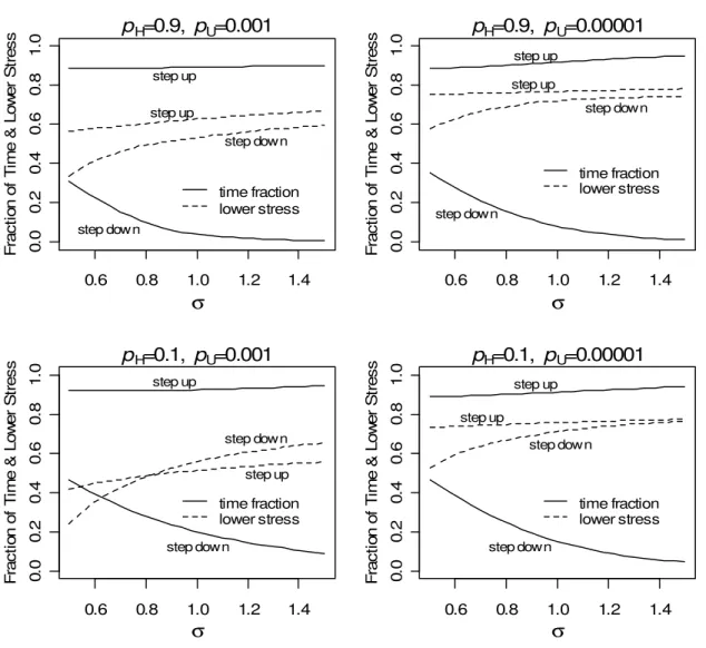
Besides theoptimum variance shown in Figures 2.1 and 2.2, it is also interesting to look at the time fraction and the lower level of stress under the optimum conditions. Figure 2.3 shows examples of the time fraction of the first step and the lower stress for 0.01 quantile with the step-up test plan and 0.5 quantile with the step-down test plan under the Weibull distributions. The reason for choosing these two quantiles is that they can provide smaller variances than that of the corresponding quantiles of a constant-stress test plan in some interval of σ values, as seen in Figure 2.1.

Figure 2.3 shows that the time fraction and lower stress change as σ changes under the optimum step-stress test plans. Concerning the possible uncertainty of the planning value of σ, one would prefer that the change of the time fraction and lower stress be as small as possible within the range of the σ uncertainty. Note that a constant-stress plan does not depend on σ. Under certain circumstances, it is possible that a substantial change in the time fraction or the lower stress may not lead to a large change in Avar(yˆ_p), if this function is very flat around the optimum point. In practice, one should assess the robustness of step-stress test plans relative to the uncertainty in σ .

The change of the time fraction and lower stress as a function of σ is not always smooth like in Figure 2.3. In some situations, these functions can have a jump change across certain σ values due to the multiple optima of the objective variance function.

(32)

0.6 0.8 1.0 1.2 1.4 0 .0 0 .2 0 .4 0 .6 0 .8 1 .0 p_H=0.9, p_U=0.001 step up step up step down step down time fraction lower stress σ F ra c ti o n o f T im e & L o w e r S tr e s s 0.6 0.8 1.0 1.2 1.4 0 .0 0 .2 0 .4 0 .6 0 .8 1 .0 p_H=0.9, p_U=0.00001 step up step up step down step down time fraction lower stress σ F ra c ti o n o f T im e & L o w e r S tr e s s 0.6 0.8 1.0 1.2 1.4 0 .0 0 .2 0 .4 0 .6 0 .8 1 .0 pH=0.1, pU=0.001 step up step up step down step down time fraction lower stress σ F ra c ti o n o f T im e & L o w e r S tr e s s 0.6 0.8 1.0 1.2 1.4 0 .0 0 .2 0 .4 0 .6 0 .8 1 .0 pH=0.1, pU=0.00001 step up step up step down step down time fraction lower stress σ F ra c ti o n o f T im e & L o w e r S tr e s s

Figure 2.3: The optimum time fraction of the first step and the lower stress for the 0.01 quantile of

step-up plan and the 0.5 quantile of step-down plan for the Weibull distribution as a function of σunder the

(33)

2.5 Some Concerns in Practical Applications

2.5.1 Avoiding plans with a small expected number of failures

The optimum time fraction and lower stress under the optimum conditions of step-stress test plans are obtained under the assumption of an infinitely large sample. In some cases, the time fraction of a step of stress can be close to zero, which means that the optimum test plans are impractical. This is because for a large-sample approximate variance to provide an adequate approximation, one needs to have a sufficiently large number of failures in each step of stress. If a step is too short, a very large number of sample units will be required to generate a sufficiently large number of failures. To avoid this problem, one can use a constraint: the time fraction of each step must be within, say, 5% and 95% of the total test time. A similar constraint also can be applied to the standardized lower stress. The actual values of the constraints should be determined in each specific situation.

In the rest of this paper, we use the 5%-95% constraint for both time fraction and lower stress. With this constraint, we reproduced results like those in Figures 2.1 and 2.2. These results (details not given here) show that imposing such constraints may, as expected, increase the variance somewhat. For example, at σ = 1.5, without the constraint, the

optimum variances of the 0.1 quantile for step-down under the Weibull distribution are 86.91 and 272.82 for pU = 0.001 and 0.00001, respectively. With the constraint, the corresponding optimum variances increase to 96.17 and 277.41 for pU = 0.001 and 0.00001, respectively.

(34)

2.5.2. Effect of misspecification of the

σ

planning value

Section 2.4.2 indicates that different σ planning values will result in different optimum test plans. Thus, it is interesting to investigate the change in Avar(yˆ_p) due to the misspecification of the σ planning value.

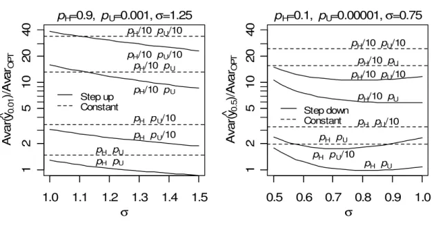
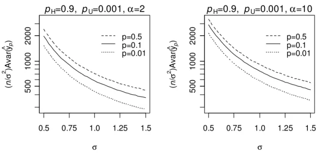
Figure 2.4 shows the ratioAvar(yˆ_p) Avar_OPTon a log scale as a function of σ for the Weibull distribution and four different sets of possible true failure probabilities under the fixed optimum step-stress test plans with Avar_OPT being Avar(yˆ_p). The left side of Figure 2.4 is for a step-up plan for the 0.01 quantile optimized at p_H = 0.9,p_U = 0.001 and σ = 1.25. The right side of Figure 2.4 is for a step-down plan for the 0.5 quantile optimized at p_H

= 0.1,p_U = 0.00001 and σ = 0.75. For simplicity, we assume the uncertainty range of the planning values of p_H , p_U and σ are [pH/10, min(10pH , 1)], [pU /10, min(10pU,pH)] and [σ −0.25, σ +0.25], respectively. Figure 2.4 provides four curves for each test plan corresponding to four possible true parameters: (p_H ,p_U), (p_H/10,p_U), (p_H ,p_U /10) and (p_H/10,p_U /10). The four straight horizontal lines are the relative variances of the

corresponding optimum constant-stress plans for the four situations. Because our primary concern is the variance increment, the cases involving 10p_H and 10p_U are omitted because they have smaller variance than those involving p_H/10 and p_U /10.

(35)

pH=0.9, pU=0.001, σ=1.25 1 2 5 1 0 2 0 4 0 1.0 1.1 1.2 1.3 1.4 1.5 Step up Constant pH pU pH pU pH pU/10 pH pU/10 pH/10 pU pH/10 pU pH/10 pU/10 pH/10 pU/10 σ A v a r( y^0.0 1 )/ A va rOP T pH=0.1, pU=0.00001, σ=0.75 1 2 5 1 0 2 0 4 0 0.5 0.6 0.7 0.8 0.9 1.0 Step down Constant p_H p_U/10 pH pU pH pU/10 pH pU p_H/10 p_U/10 pH/10 pU pH/10 pU/10 pH/10 pU σ A v a r( y^0.5 )/ A va rOP T

Figure 2.4: The ratio Avar(y ) Avarˆp OPT on a log scale as a function of σ for the Weibull distribution

and four different sets of possible true failure probabilities under fixed optimum step-stress test plans

with Avar_OPT being Avar(yˆp). On the left side is a step-up test plan for the quantile p = 0.01 optimized

at p_H = 0.9,p_U = 0.001 and σ= 1.25. On the right side is a step-down test plan for the quantile p = 0.5

optimized at p_H = 0.1,p_U = 0.00001 and σ= 0.75. The straight horizontal lines are the relative

variances of the corresponding optimum constant-stress plans. The labels on the lines indicate the perturbed true values of the failure probabilities.

Figure 2.4 demonstrates that it is useful to assess robustness to uncertainty in σ . Whether uncertainty in σ seriously affects the test plan or not depends on each specific situation. Figure 2.4 shows that, for some values of σ , optimum step-stress test plans can have smaller variance than that of the corresponding optimum constant stress plans. If, however, there is a very large amount of uncertainty in σ , a constant-stress plan might be preferable.

(36)

2.5.3 Compromise test plans

Test plans with three stress levels are often used to gain robustness to the uncertainty of planning values and verify the linear relationship of the location and the standardized stress. Meeker and Hahn [7] proposed a 4:2:1 compromise constant-stress test plan that has been widely applied, where 4, 2 and 1 represent the relative proportions of unit allocations at the low, middle and high levels of stresses, respectively.

In this section, we investigate the relationship between the minimum value of

(

_σ2

)

n Avar(yˆ_p) and σ under compromise test plans involving three stress levels. For constant-stress plans, we follow Meeker and Escobar (chapter 20 of [8]) and constrain 15% of the units to be tested at a point halfway between the highest level of stress and the lowest level of stress. The lowest level of stress and the unit allocation at this level are optimized with respect to the large sample approximate variance. Without such a constraint, in any practical situation when optimizing, the 3-level plan will degenerate to a 2-level plan. For step-stress compromise test plans with h = 3, we use a similar constraint, where 15% of the test time is spent at a level of stress halfway between the highest level of stress and the lower level of stress. The lowest level of stress and the test time at this level are optimized using the variance objective function in Section 2.3.3. Again, without such a constraint, in any

practical situation, an optimum h≥3 plan will degenerate to an h = 2 plan. Note that the 5-95% constraint described in Section 2.5.1 for unit allocation, time fraction and lower stress still hold. For simplicity, the step stress plans considered here are either straight step up or straight step down in stress.

Figures 2.5 and 2.6 show the value of scaled variance

(

_σ2

)

n Avar(yˆ_p) obtained from optimum ALT plans involving three stresses as a function of σ for three different quantiles of interest: 0.01, 0.10 and 0.50, respectively, for the Weibull and lognormal distributions. These figures also compare constant-stress, step-up-stress, and

(37)

step-down-stress test plans for different values of p_H andp_U under the Weibull and lognormal distributions, respectively. Comparing with the results in Figures 2.1 and 2.2, the scaled variance for the test plans with three stress levels have the σ dependence similar to that involving just two stress levels.

p_H=0.9, p_U=0.001 Step Up Step down Constant 6 0 1 0 0 2 0 0 5 0 0 0.5 0.75 1.0 1.25 1.5 0.1 0.01 0.5 0.1 0.01 0.5 0.5 0.1 0.01 σ ( n / σ 2 )A v a r( y^p ) p_H=0.9, p_U=0.00001 Step Up Step down Constant 3 0 0 5 0 0 1 0 0 0 0.5 0.75 1.0 1.25 1.5 0.5 0.01 0.1 0.1 0.01 0.5 0.5 0.1 0.01 σ ( n / σ 2 )A v a r( y^p ) pH=0.1, pU=0.001 Step Up Step down Constant 1 0 0 0 2 0 0 0 4 0 0 0 0.5 0.75 1.0 1.25 1.5 0.5 0.1 0.01 0.5 0.1 0.01 0.5 0.1 0.01 σ ( n / σ 2 )A v a r( y^p ) pH=0.1, pU=0.00001 Step Up Step down Constant 2 0 0 0 5 0 0 0 1 0 0 0 0 2 0 0 0 0 0.5 0.75 1.0 1.25 1.5 0.5 0.1 0.01 0.5 0.1 0.01 0.5 0.1 0.01 σ ( n / σ 2 )A v a r( y^p )

Figure 2.5: Scaled optimum variance as a function of σ for the Weibull distribution at three quantiles

of interest for four combinations of planning values under three test plans. The three quantiles of interest

(38)

The three test plans investigated are the three-stress-level step-up stress, step-down stress and constant stress, respectively. p_H=0.9, p_U=0.001 Step-up Step-down Constant 1 0 2 0 5 0 1 0 0 0.5 0.75 1.0 1.25 1.5 0.5 0.01 0.1 0.5 0.1 0.01 0.5 0.1 0.01 σ ( n / σ 2 )A v a r( y^p ) p_H=0.9, p_U=0.00001 Step Up Step down Constant 2 0 5 0 1 0 0 2 0 0 0.5 0.75 1.0 1.25 1.5 0.01 0.5 0.1 0.5 0.1 0.01 0.1 0.5 0.01 σ ( n / σ 2 )A v a r( y^p ) pH=0.1, pU=0.001 Step Up Step down Constant 1 0 0 2 0 0 5 0 0 2 0 0 0 0.5 0.75 1.0 1.25 1.5 0.1 0.01 0.5 0.1 0.01 0.5 0.01 0.1 0.5 σ ( n / σ 2 )A v a r( y^p ) pH=0.1, pU=0.00001 Step Up Step down Constant 3 0 0 5 0 0 1 0 0 0 2 0 0 0 0.5 0.75 1.0 1.25 1.5 0.5 0.1 0.01 0.5 0.1 0.01 0.01 0.1 0.5 σ ( n / σ 2 )A v a r( y^p )

Figure 2.6: Scaled optimum variance as a function of σ for the lognormal distribution at three quantiles

of interest for four combinations of planning values under three test plans. The three quantiles of interest

0.001), (p_H = 0.9, p_U = 0.00001), (p_H = 0.1, p_U = 0.001) and (p_H = 0.1, p_U = 0.00001), respectively.

The three test plans investigated are the three-stress-level “compromise” step-up stress, step-down stress and constant stress, respectively.

(39)

2.6 Adequacy of the Large Sample Approximate Variance

In practical applications, simulation is frequently used to complement evaluations

done with large-sample approximations (e.g., Chapter 6 of [12] or Chapter 20 of [8]) to evaluate test plans design. Here we provide some results of such simulations.

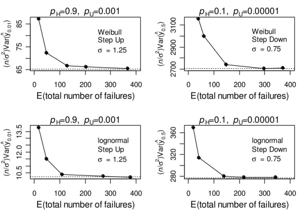
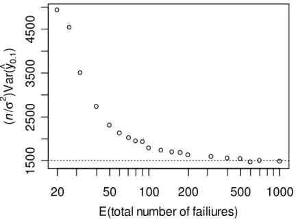
Figure 2.7 shows the simulated scaled variance as a function of the expected total number of failures under four optimum stress-test test plans, compared with the large-sample approximation. As expected, when the expected total number of total units gets large, the simulated variance becomes close to the large-sample approximate variance. The results are presented in terms of the expected number of failures instead of sample size because, as is true in other similar situations involving censored data, the adequacy of the large-sample approximation is approximately a function of the expected number of failures, rather than the actual sample size (notice that the shapes of the functions in Figure 2.7 are all similar).

(40)

0 100 200 300 400 6 5 7 5 8 5 p_H=0.9, p_U=0.001 Weibull Step Up σ = 1.25

E(total number of failures)

( n / σ 2 )V a r( y^0 .0 1 ) 0 100 200 300 400 2 7 0 0 2 9 0 0 3 1 0 0 pH =0.1, p_U=0.00001 Weibull Step Down σ = 0.75

( n / σ 2 )V a r( y^0 .5 ) 0 100 200 300 400 1 0 .5 1 2 .0 1 3 .5 pH=0.9, pU=0.001 lognormal Step Up σ = 1.25

( n / σ 2 )V a r( y^0.0 1 ) 0 100 200 300 400 2 8 0 3 2 0 3 6 0 pH=0.1, pU=0.00001 lognormal Step Down σ = 0.75

( n / σ 2 )V a r( y^0 .5 )

Figure 2.7: Simulated scaled variance as a function of the expected total number of failures under optimum stress-test test plans (large dots with solid lines for visual guidance) compared with the large-sample approximation (horizontal dashed line). The number of simulations at each point is 20,000.

While simulation methods are useful, the amount of computer time needed to do an evaluation of a particular test plan will take orders of magnitude longer that the large-sample approximate variance method. For example, given planning valuesp_H , p_U and σ to be 0.1, 0.001 and 0.8, respectively, and a plan with 1000 test units, it took approximately 42 seconds to evaluate a particular step-up test plan under the Weibull distribution on a typical desktop computer with a 2.4GHz processor. The analytical large sample approximation can be computed more than 1000 times faster. For this reason, an extensive study of optimum test plans is not really practicable when using simulation to do evaluations. On the other hand, graphical presentation of simulation results can generally give a much better approximation to the true variances (limited only by Monte Carlo error) and provide detailed information

(41)

and additional insight about test plan properties as well as the verification of the analytical approach.

2.7 Concluding Remarks and Areas for Future Research

This paper extends previous work that has been done on planning step-stress ALTs. We give a general approach for computing the large-sample approximate variance of ML estimators of quantiles of interest under the widely used log-location-scale family of distributions for multi-step-stress ALTs with censoring. The approach allows comparison among different test plans under different assumed log location-scale distributions.

Comparison of step-stress test plans shows that the scaled optimum variance

decreases as σ increases. In terms of the scaled optimum variance, the simple step-down test plan usually performs better than the simple step-up test plan when the failure probability at the level of the highest stress is small.

Compared with step-stress test plans, the above results show that, when both time/allocation fraction and lower stress are optimized, constant-stress plans are a good choice when σ is small and p_H is not too small. This is because constant-stress plans usually provide test plans with a smaller optimum variance of the ML estimators. Step stress plans can have a smaller optimum variance than constant stress plans when σ is large or whenp_H is very small (as it often is in practice).

Although the numerical results in this paper are focused on the comparison among simple constant-stress test plans and step-stress test plans, the approach given here provides a way to evaluate and compare a variety of more complicated multi-step-stress test plans for any log-location-scale distribution. Possible areas for future research include

(42)

• Extension to some other non-log-location-scale distributions and other

time-dependent stress levels than step stress under general log-location-scale distributions.

• Exploration of other step-stress test plans not studied in this paper that might provide

robustness to the uncertainty of planning values or the possible departure from log linear location-stress model.

• Application of step-stress methods to accelerated tests that provide degradation data.

Appendix

This appendix provides the derivatives of the log likelihood described in Section 2.3 and the details of the approach that we used to calculate the large-sample approximate variance-covariance matrix of the ML estimators of γ₀, γ₁ and σ . For a log-location-scale distribution, we have the following properties

σ γ 1 0 − = ∂ ∂zi , σ σ i i z z − = ∂ ∂ and zi

(

_ν_i _ξ_i

)

σ γ = − ∂ ∂ 1 1 , where

∑

(

)(

)

( )

(

)

− = − − − − − − = 1 1 1 1 / 1 i j i j i j j i e t j i

δ

ξ

τ

ν

γ ξ ξ , i₌2,3,K,h_{. Let} ₍ ₎ ₀ 1 t = ν and ν_η

is νh at t=η. ziis defined in Section 2.2. The step-up test plan results in a positiveνi, while the step-down results in a negative ν_i; for constant stress, ν_i= 0, i₌2,3,K,h_{. This leads to}

dramatic differences in the properties of optimum ALT among these three test plans.

By means of the above properties, for a log-location-scale distribution, the first partial derivatives with respect to parameters of the log likelihood for a single observation can be expressed as         Φ ⋅ Φ − − ⋅ − = ∂ ∂

∑

= + h i h i i i dz z d z t U dz z d z t U l 1 1 0 ) ( ) ( 1 1 ) ( ) ( ) ( 1 ) ( 1 η η φ φ σ γ

(43)

(

)

(

)

        − Φ ⋅ Φ − +       − ⋅ − − = ∂ ∂

∑

= + h i h h i i i i i i dz z d z t U dz z d z t U l 1 1 1 ) ( ) ( 1 1 ) ( ) ( ) ( 1 ) ( 1 ξ ν ξ ν φ φ σν σ γ η η η         Φ ⋅ Φ − −       ⋅ + − = ∂ ∂

∑

= + h i h i i i i dz z d z z t U dz z d z z t U l 1 1 ) ( ) ( 1 ) ( ) ( ) ( 1 ) ( 1 η η η φ φ σ σ . Define = ) (z A 2 2 2 2 ₍ ₎ ) ( 1 ) ( ) ( 1       ⋅ − ⋅ dz z d z dz z d z φ φ φ φ ,

[

]

2 2 2 2 ) ( ) ( 1 1 ) ( ) ( 1 1 ) (       Φ ⋅ Φ − + Φ ⋅ Φ − = dz z d z dz z d z z B .

Note that the first partial derivatives are zero when evaluated at ML estimates when they are not on the boundary of the parameter space. We set terms corresponding to the first partial derivatives equal to zero in the following expressions for the second partial

derivatives of the log likelihood. The resulting second partial derivatives of the log likelihood for a single observation, evaluated at the ML estimates are:

      − = ∂ ∂

∑

= + h i t h i i t A z U t B z U l 1 1 2 2 0 2 ) ( ) ( ) ( ) ( 1 σ γ .

(

)

              − + ⋅ + − = ∂ ∂

∑

= h i i i i i i i i i A z dz z d z t U l 1 2 2 2 2 1 2 ) ( ) ( ) ( 1 ' ' ) ( 1 ξ ν φ φ σν ν σ σ γ

(

)

        − + Φ ⋅ Φ − − + ) ( ) ( ) ( 1 1 ' ) ( 2 2 1 η η η η η ν ξ σν σ dz B z z d z t U h h

[

]

      − + − = ∂ ∂

∑

= + h i h i i i t z A z U t z B z U l 1 2 1 2 2 2 2 ) ( ) ( ) ( 1 ) ( 1 η η σ σ       − = ∂ ∂ ∂

∑

= + h i h i i i t z A z U t z B z U l 1 1 2 0 2 ) ( ) ( ) ( ) ( 1 η η σ γ σ

(

)

(

)

      − + − ⋅ = ∂ ∂ ∂

∑

= + h i h h i i i i t A z U B z U l 1 1 2 0 1 2 ) ( ) ( ) ( 1 η η ξ ν ν ξ σ γ γ

(

)

[

]

(

)

      ⋅ − + ⋅ − − − = ∂ ∂ ∂

∑

= + h i h h i i i i i i t z A z U t z B z U l 1 1 2 1 2 ) ( ) ( ) ( ) ( 1 η η η ξ ν ξ ν σν σ σ γ ,

(44)

where

∑

(

)(

)

( )

(

)

− = − − − − − − − = ∂ ∂ = 1 1 2 1 2 1 1 / / ' 1 i j i i j i j j i i e t j i _δ _ν ξ ξ τ τ γ ν ν γ ξ ξ , νη'=νh'

( )

η and h i₌2,3,K, _.

Let θ =

(

γ₀,γ₁,σ

)

. The Fisher information matrix of a step-stress ALT can be

computed as _      ∂ ∂ ∂ − =E l

New Developments in Planning Accelerated Life Tests