MPRA
Munich Personal RePEc Archive
Strict stationarity testing and estimation
of explosive ARCH models
Christian Francq and Jean-Michel Zakoian
April 2010
Online at
http://mpra.ub.uni-muenchen.de/22414/
explosive ARCH models
By Christian Francq∗University Lille 3, EQUIPPE-GREMARS and
By Jean-Michel Zakoïan∗ CREST and University Lille 3
This paper studies the asymptotic properties of the quasi-maximum likelihood estimator of ARCH(1) models without strict stationarity constraints, and considers applications to testing prob-lems. The estimator is unrestricted, in the sense that the value of the intercept, which cannot be consistently estimated in the explosive case, is not fixed. A specific behavior of the estimator of the ARCH coefficient is obtained at the boundary of the stationarity region, but this estimator remains consistent and asymptotically normal in ev-ery situation. The asymptotic variance is different in the stationary and non stationary situations, but is consistently estimated, with the same estimator, in both cases. Tests of strict stationarity and non stationarity are proposed. Their behaviors are studied under the null assumption and under local alternatives. The tests developed for the ARCH(1) model are able to detect non-stationarity in more general GARCH models. A numerical illustration based on stock indices is proposed.
1. Introduction. Testing for strict stationarity is an important issue in the context of financial time series. A standard assumption is that the prices are non stationary while the returns (or log-returns) are stationary. Numer-ous statistical tools, such as the unit root tests, have been introduced for test-ing the non-stationarity of prices. For the log-returns, the most widely used models are arguably the GARCH introduced by Engle (1982) and Bollerslev (1986). No statistical tools are available for testing strict stationarity in the GARCH framework. This is the main aim of this paper to develop such tools. The problem is non standard because, contrary to stationarity in linear time
∗The authors are very grateful to Professor Y. Davydov and to Professor L. Horváth
for stimulating and instructive discussions on topics related to this paper. AMS 2000 subject classifications:Primary 62M10; secondary 62F12, 62F05.
Keywords and phrases:ARCH model, Inconsistency of estimators, Local power of tests, Nonstationarity, Quasi Maximum Likelihood Estimation
series models, which solely depends on the lag polynomials, the strict sta-tionarity condition for GARCH models has a non explicit form, involving the distribution of the underlying independent and identically distributed (iid) sequence.
The asymptotic properties of the quasi-maximum likelihood estimator (QMLE) for classical GARCH models have been extensively studied; see Berkes, Horváth and Kokoszka (2003), Francq and Zakoïan (2004) and the references therein. For valid statistical inference based on those results, strict stationarity must hold. Thus, from the point of view of the validity of the asymptotic results for the QMLE, strict stationarity testing in GARCH mod-els is also an important issue. Surprisingly, this issue has not been addressed in the literature, to the best of our knowledge.
1.1. Modes of divergence in the non stationary case. The complexity of the statistical problem arises from the specificities of the probabilistic framework, even for the simplest GARCH model. To fix ideas, consider the ARCH(1) model, given by
(1.1)
(
ǫt=√htηt, t= 1,2, . . .
ht=ω0+α0ǫ2t−1
with an initial value ǫ0, where ω0 > 0, α0 ≥ 0, and (ηt) is a sequence of
independent and identically distributed (iid) variables such that Eη1 = 0
and Eη2
1 = 1. The necessary and sufficient condition for the existence of a
strictly stationary solution to (1.1) is (by Nelson, 1990)
(1.2) γ0<0 (i.e. α0 <exp
n
−Elogη12o), where γ0 =Elog(α0η12). More precisely, if (1.2) holds we have
(1.3) ht−σt2→0 almost surely ast→ ∞, where (1.4) σt2= lim n→∞↑σ 2 t,n, σt,n2 =ω0 1 + n−1 X k=1 αk0ηt2−1. . . η2t−k ! . Let us now turn to the nonstationary case, for which it is necessary to con-sider separatelyγ0>0 and γ0 = 0. Under the assumption
(1.5) γ0>0 (i.e. α0 >exp
n
ht → ∞ almost surely as t→ ∞, as shown by Nelson (1990). In this case,
the increasing sequenceσ2
t,n goes to infinity almost surely ast→ ∞, by the
Cauchy root test. The case γ0 = 0 is much more intricate. By the
Chung-Fuchs theorem, it can be seen that σt,n2 goes to infinity almost surely as t → ∞. However, (1.3) may not hold when γ0 = 0. Actually, Klüppelberg,
Lindner and Maller (2004) (see also Goldie and Maller (2000)) showed that
(1.6) when γ0 = 0, ht→ ∞ in probability
instead of almost surely in the case γ0 > 0 1. The astonishing difficulties
encountered in the case γ0 = 0 are related to the fact that the sequence
ht=σ2t,t+αt0η2t−1. . . η21ǫ20 does not increase witht.
1.2. The statistical problem. Denote byθ= (ω, α)′ the ARCH(1) param-eter and define the QMLE as any measurable solution of
(1.7) θˆn= (ˆωn,αˆn)′ = arg min θ∈Θ 1 n n X t=1 ℓt(θ), ℓt(θ) = ǫ2t σ2 t(θ) + logσ2t(θ),
whereΘis a compact subset of(0,∞)2, andσ2
t(θ) =ω+αǫ2t−1fort= 1, . . . , n
(with an initial value forǫ20). The rescaled residuals are defined byηˆt=ηt(ˆθn)
where ηt(θ) =ǫt/σt(θ) for t= 1, . . . , n.
To construct a test of the strict stationarity assumption, we will establish the asymptotic distribution, under (1.2), of the statistic
ˆ γn= log ˆαn+ 1 n n X t=1 log ˆη2t.
This will be accomplished by deriving the joint distribution of (ˆαn,n1Pnt=1log ˆηt2), under the assumptions used to prove the asymptotic
normality of the QMLE θˆn.
To study the asymptotic power of the test, it is necessary to analyze the asymptotic behavior of the QMLE whenγ0≥0.Jensen and Rahbek (2004a,
2004b) were the first to establish an asymptotic theory for estimators of
non-stationary GARCH. 2 They considered a constrained QMLE of α
0 (in
the sense that the value of the intercept is fixed) which is consistent in the non stationary case, but is inconsistent in the stationary case. We will estab-lish the strong consistency and asymptotic normality of the (unconstrained)
1
Klüppelberg, Lindner and Maller (2004) noted that the arguments given by Nelson (1990) for the a.s. convergence are in failure whenγ0= 0.
2
QMLE of α0, the only component which matters for our testing problem,
when γ0 >0. It turns out that, contrary to the strict stationarity case, the
asymptotic distribution of αˆn is extremely simple, and is given by
√ n(ˆαn−α0)→ Nd n 0,(κη −1)α20 o , asn→ ∞
where→d stands for the convergence in distribution. Whenγ0= 0, the QMLE
ofα0 will be shown to be weakly consistent with the same asymptotic normal
distribution as in the case γ0 > 0. The asymptotic variances of αˆn when
γ0 ≥0and whenγ0<0do not coincide, but we propose an estimator which
is consistent in both situations. This is in accordance with similar results for autoregressive models with random coefficients derived by Aue and Horváth (2009).
The rest of the paper is organized as follows. Section2 is devoted to the asymptotic properties of the QMLE. In Section3, we first consider the prob-lem of testing the value of α without any stationarity restriction. Then, we consider strict stationarity testing. The asymptotic distributions of two tests are studied when the null assumption is either the stationarity or the non sta-tionarity. Section4is devoted to a power study. We start by establishing the Local Asymptotic Normality (LAN) of the ARCH(1) model without station-arity. The Fisher information matrix is degenerate in the caseγ0 ≥ 0. The
LAN property is used to derive the local asymptotic power of the proposed tests. Optimality issues are discussed. Necessary and sufficient conditions on the noise density are derived for the tests to be uniformly locally asymptot-ically most powerful. We also consider testing stationarity in more general GARCH-type models. Numerical illustrations are provided in Section 6. In particular, the stationarity of eleven major stock returns is analyzed. Proofs and complementary results, in particular the inconsistency of the constrained estimators in the stationary case, are collected in Section7.
2. Asymptotic properties of the QMLE. In this paper we consider the standard QMLE, which is the commonly used estimator for GARCH models.
2.1. Consistency and asymptotic normality of αˆn. The following result
completes those already established in the stationary case, which we recall for convenience. The asymptotic distribution in the case γ0 = 0 will be treated
separately.
Theorem 2.1. For the ARCH(1) model (1.1), let the QMLE defined in (1.7).
i) When γ0 <0 and P(ηt2= 1)<1 ˆ αn→α0 and ωˆn→ω0 a.s. asn→ ∞. ii) When γ0 >0, ˆ αn→α0 a.s. asn→ ∞. iii) When γ0 = 0, ˆ αn→α0 in probability as n→ ∞.
iv) When γ0 < 0, κη = Eη14 ∈ (1,∞) and θ0 = (ω0, α0)′ belongs to the
interior Θ◦ of Θ, (2.1) √nθˆn−θ0 d → Nn0,(κη −1)J−1 o , as n→ ∞, and (2.2) J =E 1 (ω0+α0ǫ21)2 ǫ2 1 (ω0+α0ǫ21)2 ǫ2 1 (ω0+α0ǫ21)2 ǫ4 1 (ω0+α0ǫ21)2 . v) When γ0 >0, κη ∈(1,∞) and θ0∈ ◦ Θ, (2.3) √n(ˆαn−α0)→ Nd n 0,(κη −1)α20 o , asn→ ∞.
To obtain the asymptotic distribution of αˆn in the case γ0 = 0, we need
an additional assumption on the distribution of η2t. Let Zt = α0ηt2. Note
thatγ0 =ElogZt= 0entails E(1 +Zt−1+Zt−1Zt−2+· · ·+Zt−1. . . Z1)≥t
by Jensen’s inequality. We introduce the assumption
A:when ttends to infinity,
E 1 1 +Z1+Z1Z2+· · ·+Z1. . . Zt−1 =o 1 √ t .
Note thatAis obviously satisfied when Zt= 1a.s., since the expectation is
then equal to1/t.
Theorem 2.2. Suppose that γ0 = 0, θ0 ∈
◦
Θ, κη ∈ (1,∞) and A is
satisfied. Then the QMLE αˆn is asymptotically normal and its asymptotic
2.2. Estimator of the asymptotic variance of αˆn with or without
station-arity. In view of (2.1)-(2.2), whenγ0 <0the asymptotic distribution of the
QMLEαˆn of θ0 is given by (2.4) √n( ˆαn−α0)→ N {d 0,(κη−1)ξ}, asn→ ∞, with (2.5) ξ = µ(0,2) µ(0,2)µ(2,2)−µ2(1,2), µ(p, q) =E ǫ21p (ω0+α0ǫ21)q . It is obvious to show that the empirical estimator ofξ
ˆ ξn= ˆ µn(0,2) ˆ µn(0,2)ˆµn(2,2)−µˆ2n(1,2) , where µˆn(p, q) = 1 n n X t=1 ǫ2tp (ˆωn+ ˆαnǫ2t)q , is strongly consistent in the stationary case γ0 < 0. The following result
shows that this estimator is also a consistent estimator of the asymptotic variance ofαˆn in the nonstationary case γ0≥0.
Theorem 2.3. Assume θ0 ∈Θ, κη ∈(1,∞) and let κˆη =n−1Pnt=1ηˆt4,
where ηˆt=ǫt/σt(ˆθn).
i) When γ0 <0, we have ˆκη →κη andξˆn→ξ a.s as n→ ∞.
ii) When γ0 >0, we have ˆκη →κη andξˆn→α20 a.s.
iii) When γ0 = 0, we have ˆκη → κη and, if A is satisfied, ξˆn → α20 in
probability.
In any case, (ˆκη −1)ˆξn is a consistent estimator of the asymptotic variance
of the QMLE of α0.
The consequence of Theorem 2.3, from a practical point of view, is ex-tremely important. It means that we can get confidence intervals, or tests forα0 without assuming stationarity/nonstationarity.
3. Testing. Before considering strict stationarity testing, we start with tests on the parameterα.
3.1. Testing the ARCH coefficient. Consider a testing problem of the form
(3.1) H0 : α0 ≤α∗ against H1 : α0> α∗,
whereα∗is a given positive number. A value of particular interest isα∗ = 1, becauseEǫ2
any constraint on α∗ so that some values of α0 ≤ α∗ may correspond to
nonstationary ARCH models. A direct consequence of Theorems2.1-2.2-2.3
is the following result, in whichΦdenotes theN(0,1)cumulative distribution function. Letα∈(0,1).
Corollary 3.1. Assume that θ0 ∈
◦
Θ and the assumptions of Theorem
2.3hold. For the testing problem (3.1), the test defined by the critical region
(3.2) Cα∗ = Tnα∗ := √ n(ˆαn−α∗) q (ˆκη −1)ˆξn >Φ−1(1−α)
has the asymptotic significance level α and is consistent.
Hence, assumption H0 can be tested without knowing if the observations
are generated by a stationary or an explosive ARCH. However, it is of interest to test if a given series is stationary or not. This cannot be done by testing an assumption of the form (3.1).
3.2. Strict stationarity testing. Consider the strict stationarity testing problems (3.3) H0 :γ0 <0 against H1 :γ0 ≥0, and (3.4) H0 :γ0 ≥0 against H1 :γ0 <0, where γ0 = Elog α0η21
. These hypotheses are not of the form (3.1)
because γ0 not only depends on α0, but also on the unknown moment
ζ := Elogηt2 ∈ R∪ {−∞}. Let ζˆn = n−1Pnt=1log ˆηt2. The following
re-sult gives the asymptotic joint distribution ofζˆnandαˆn, and the asymptotic
distribution of a consistent estimator of γ0, under either the stationarity or
the nonstationarity conditions.
Theorem 3.1. Assume that Eη41 ∈(1,∞),E
logη12 2 <∞ andθ0 ∈ ◦ Θ. i) If the stationarity condition γ0<0 holds, as n→ ∞,
(3.5) √ n ˆζˆn−ζ θn−θ0 ! d → N ( 0,Σ := σu2+σv2+ 2σuv −(σ2v+σuv)θ0′ −(σ2v+σuv)θ0 σ2vJ−1 !) ,
where vt = 1−ηt2, σv2 = Evt2, ut = logη2t −ζ, σu2 = Eu2t, σuv =
Cov(ut, vt) and J is given by (2.2). Moreover
(3.6) γˆn := ˆζn+ log ˆαn→γ0 in probability as n→ ∞ and (3.7) √n(ˆγn−γ0)→ Nd 0, σu2+σ2v ξ α20 −1 as n→ ∞.
ii) If γ0 >0, or if γ0 = 0 and A holds, then
(3.8) √ n ζˆn−ζ ˆ αn−α0 ! d → N ( 0, σu2+σv2+ 2σuv −(σ2v+σuv)α0 −(σ2 v +σuv)α0 σv2α20 !) .
Moreover (3.6) holds and we have
(3.9) √n(ˆγn−γ0)→ Nd
0, σu2 asn→ ∞.
It is interesting to note that the asymptotic distribution ofζˆn is the same
in the cases γ0 <0 and γ0 ≥0 and that this distribution is independent of
θ0.
Letσˆu2 =n−1Pnt=1 log ˆηt22
−ζˆn2.
Corollary3.2. Let the assumptions of Theorem3.1hold. For the test-ing problem (3.3), the test defined by the critical region
(3.10) CST = Tn:=√n ˆ γn ˆ σu >Φ−1(1−α)
has its asymptotic significance level bounded by α, has the asymptotic prob-ability of rejection α under γ0 = 0, and is consistent for all γ0 >0.
For the testing problem (3.4), the test defined by the critical region
(3.11) CNS=nTn<Φ−1(α)
o
has its asymptotic significance level bounded by α, has the asymptotic prob-ability of rejection α under γ0 = 0, and is consistent for all γ0 <0.
4. Asymptotic local powers. The section investigates the asymptotic behavior under local alternatives of the tests (3.2) on α0 and of the strict
stationarity tests (3.10) and (3.11). We first establish the LAN of the ARCH model without imposing any stationarity constraint. This LAN property will
be used to derive the asymptotic properties of our tests, but the result is of independent interest (see van der Vaart (1998) for a general reference on LAN and its applications, and see Drost and Klaassen (1997), Drost, Klaassen and Werker (1997) and Ling and McAleer (2003) for applications to GARCH and other stationary processes).
4.1. LAN without stationarity constraint. Assume that ηt has a density
f with third-order derivatives, that
(4.1) lim
|y|→∞y
2f′(y) = 0,
and that for some positive constantsK and δ
(4.2) |y| f′ f (y) +y 2 f′ f ′ (y) +y2 f′ f ′′ (y) ≤K1 +|y|δ, (4.3) E|η1|2δ<∞.
These regularity conditions are satisfied for numerous distributions, in par-ticular for the gaussian distribution withδ = 2, and entail the existence of the Fisher information for scale
ιf =R {1 +yf′(y)/f(y)}2f(y)dy <∞.
Given the initial valueǫ0, the density of the observations(ǫ1, . . . , ǫn)
satisfy-ing (1.1) is given byLn,f(θ0) =Qnt=1σt−1(θ0)f n σt−1(θ0)ǫt o .Aroundθ0 ∈ ◦ Θ, let a sequence of local parameters of the form θn = θ0 +τn/√n, where
(τn) is a bounded sequence of R2. Without loss of generality, assume that
n is sufficiently large so that θn ∈ Θ. Under the strict stationarity
condi-tionγ0<0, Drost and Klaassen (1997) showed that the log-likelihood ratio
Λn,f(θn, θ0) = logLn,f(θn)/Ln,f(θ0) satisfies the LAN property
(4.4) Λn,f(θn, θ0) =τn′Sn,f(θ0)− 1 2τn′Ifτn+oPθ0(1), Sn,f(θ0) d −→ N {0,If} under Pθ0 as n → ∞. The following proposition shows that (4.4) holds
regardless ofγ0.
Proposition 4.1. When θ0 ∈
◦
Θ, under (4.1)-(4.3) we have the LAN property (4.4). Whenγ0≥0, the Fisher information is the degenerate matrix
(4.5) If = ιf
4
0 0
0 α−02
4.2. Local asymptotic powers of the tests. Because the information matrix (4.5) is singular, when γ0 ≥0 the LAN property does not entail the
convo-lution theorem of Hájek (see Theorem 2.2 of Drost and Klaassen (1997)). The LAN property, with the help of Le Cam’s third lemma, allows however to easily compute local asymptotic powers of tests. In view of Corollary3.2,
lim n→∞Pθ0 CST= lim n→∞Pθ0 CNS=α,
when θ0 = (ω0, α0)′ is such that α0 = exp(−Elogηt2). Denote by Pn,τ,
whereτ = (τ1, τ2)′, the distribution of the observations(ǫ1, . . . , ǫn)when the
parameter is of the form ω0+τ1/√n, exp(−Elogη2t) +τ2/√n′. We should
use the notation(ǫ1,n, . . . , ǫn,n)instead of(ǫ1, . . . , ǫn)because the parameter
varies with n, but we will avoid this heavy notation. Local alternatives for theCST-test (resp. theCNS-test) are obtained for τ
2>0(resp.τ2<0).
Proposition 4.2. Under the assumptions of Theorem 3.1 and Propo-sition4.1, the local asymptotic powers of the strict stationarity tests (3.10) and (3.11) are given by
(4.6) lim n→∞Pn,τ CST= Φ τ 2 α0σu − Φ−1(1−α) and lim n→∞Pn,τ CNS= Φ Φ−1(α)− τ2 α0σu .
We now compute the local asymptotic power of the test defined by (3.2). We thus consider a sequence of local parameters of the formθnα∗ = (ω0, α∗)′+
τ /√nwhereτ = (τ1, τ2)′ withτ2 >0. We denote byPn,τα∗ the distribution of
the observations under the assumption that the ARCH(1) parameter isθα∗
n .
Proposition 4.3. Let the assumptions of Proposition4.1 and Theorem
2.3be satisfied. For testing (3.1), the test defined by the rejection region (3.2) has the local asymptotic power
(4.7) lim n→∞P α∗ n,τ Cα∗= Φ τ2 q (κη −1)ξ0 −Φ−1(1−α) ,
where ξ0 = α∗2 when Elogα∗η12 ≥ 0 and ξ0 = ξ defined by (2.5) when
4.3. Optimality issues. Let T2 be a subset of R containing 0. When
γ0 ≥ 0, the relations (4.4)-(4.5) imply that the limiting distribution of
Λn,f(θ0 +τ /√n, θ0) is that of the log-likelihood ratio in the statistical
model N(τ2,4α20/ιf) of parameter τ2. In other words, the so-called local
experiments {Ln,f(θ0+ (0, τ2)′/√n), τ2 ∈T2} converge to the gaussian
ex-periment
N τ2,4α20/ιf, τ2 ∈T2 (see van der Vaart (1998) for details
about the notion of statistical experiments). Testing α0 ≤ exp(−Elogη21)
against α0 > exp(−Elogη21) corresponds to testing τ2 ≤ 0 against τ2 > 0
in the limiting experiment. The uniformly most powerful test based on X ∼ N τ2,4α20/ιf is the Neyman-Pearson test of rejection region C = n
X/q4α2
0/ιf >Φ−1(1−α) o
. This optimal test has the power
(4.8) Pτ2(C) = Φ τ2 q 4α20/ιf −Φ−1(1−α) .
A test of (3.10) whose level and power jointly converge toαand to the bound in (4.8), respectively, will be called asymptotically optimal. A similar result holds for the dual testing problem (3.11). For the testing problem (3.1), the optimal local asymptotic power is
(4.9) Φ τ2 q 4ξ0/ιf −Φ−1(1−α) ,
where ξ0 is defined in Proposition 4.3.
Proposition 4.4. Under the assumptions of Proposition 4.2, the strict stationarity tests (3.10) (and/or (3.11)) is asymptotically optimal if and only if (4.10) f(y) = 1 2p |δ|πe−δ/4e (log|y|)2 δ y−2, δ <0.
The test (3.2) is optimal for the testing problem (3.1) if and only if
(4.11) f(y) = a a Γ(a)e −ay2 |y|2a−1, a >0, Γ(a) = Z ∞ 0 t a−1e−tdt.
Figure 1 displays the densities (4.11) and (4.10) for different values of a and δ. Note that the gaussian density is obtained in (4.11) for a = 1/2. The result was expected because the Cα∗-test is based on the QMLE of α0, and the QMLE is efficient in the gaussian case. Note however that the
−3 −2 −1 0 1 2 3 0.0 0.1 0.2 0.3 0.4 0.5 0.6 0.7 a=1/8 a=1/4 a=1/2 a=1 a=2 −3 −2 −1 0 1 2 3 0.0 0.2 0.4 0.6 0.8 δ=−1/8 δ=−1/4 δ=−1/2 δ=−1 δ=−2
Fig 1.Densities (4.11) ofηtfor which the test (3.2) onα0is asymptotically optimal
(left panel) and densities (4.10) for which the strict stationarity tests (3.10) and (3.11) are asymptotically optimal (right panel).
0 100 200 300 400 500 0.0 0.2 0.4 0.6 0.8 1.0 ν=2.1 0 20 40 60 80 0.0 0.2 0.4 0.6 0.8 1.0 ν=3 0 5 10 15 20 25 30 0.0 0.2 0.4 0.6 0.8 1.0 ν=10
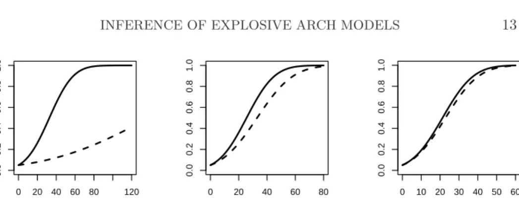
Fig 2. Optimal asymptotic power (in full line) and local asymptotic power of the strict stationarity test (3.10) (in dotted line) whenηtfollows a standardized Student
0 20 40 60 80 120 0.0 0.2 0.4 0.6 0.8 1.0 ν=4.1 0 20 40 60 80 0.0 0.2 0.4 0.6 0.8 1.0 ν=6 0 10 20 30 40 50 60 0.0 0.2 0.4 0.6 0.8 1.0 ν=10
Fig 3. Optimal asymptotic power (in full line) and local asymptotic power of the
test (3.1) (in dotted line) for testingα0< α∗ whereα∗= 2 exp(−ζ)whenηtfollows
a standardized Student distribution withν degrees of freedom.
Cα∗
-test is also asymptotically optimal when ηt follows some non gaussian
distributions. The strict stationarity tests are not optimal in the gaussian case. For densities which do not belong to the class (4.10), there is a price to pay for the estimation of ζ and/or for using an estimator of α0 which
is asymptotically less accurate than the MLE. This point is illustrated by Figures 2–3, in which the local asymptotic powers of the different tests (in dotted lines) are compared to the optimal asymptotic powers given by (4.8) and (4.9). In these two figures, the noiseηt is assumed to satisfy a Student
distribution withν >2degrees of freedom, standardized in such a way that Eη2
t = 1. Figure3considers tests of the null assumptionα0 ≤α∗, whereα∗ =
2 exp(−Elogηt2) is such that γ0 = 0 for this particular distribution. It can
be seen, in Figure3, that the local asymptotic power is far from the optimal power when ν is small, but the discrepancy decreases as ν increases. By contrast, the discrepancy increases withν in Figure2. This is not surprising since the normal distribution belongs to the class defined by (4.11), but not to that defined by (4.10).
5. Testing non stationarity in non linear GARCH. In this section we study the behaviour of the stationarity tests of Section3.2when the data are generated by the following GARCH-type model:
(5.1)
(
ǫt = √htηt, t= 1,2, . . .
ht = ω(ηt−1) +a(ηt−1)ht−1
with an initial value h0, under the same assumptions on (ηt) as in Model
(1.1). In this model, ω : R → [ω,+∞), for some ω > 0, and a: R → R+. This model belongs to the so-called class of augmented GARCH mod-els (see Hörmann, 2008) and encompasses many classes of GARCH(1,1)
models introduced in the literature: for instance, with constant ω(·), the standard GARCH(1,1) when a(x) = α0x2 + β0; the GJR model when
a(x) = α1(max{x,0})2 +α2(min{x,0})2 +β0. It can be shown that, if
Elog+a(ηt)<∞,
(5.2) Γ :=Eloga(ηt)<0
is a necessary and sufficient condition for the strict stationarity of this model (see e.g. Francq and Zakoïan, 2006a). Our aim is to test strict stationarity, without estimating the non parametric Model (5.1). We shall see that, sur-prisingly, the tests developed for the standard ARCH(1) model still work in this framework. Recall that the tests are founded on the statistics
ˆ γn= log ˆαn+ 1 n n X t=1 log ˆηt2, σˆu2 = 1 n n X t=1 log ˆηt22− 1 n n X t=1 log ˆηt2 !2
whereαˆndenotes the QMLE of the ARCH coefficient in an ARCH(1) model
and the squared rescaled residuals are given by ˆ ηt2= ǫ 2 t ˆ ωn+ ˆαnǫ2t−1 , t= 1, . . . , n.
Proposition 5.1. Let ǫ1, . . . , ǫn denote observations from Model (5.1).
Assume 0 < E|logη21|2 < ∞, E|loga(η1)|2 < ∞, Ea(η1)/η12 < ∞, and
E|ω(η1)|s <∞ for some s >0.
If Γ>0 then
ˆ
γn→Γ, and σˆ2u→Varlog η12a(η0) η2 0 >0, a.s.
If Γ<0then, under regularity conditions implying the strong consistency of θˆn to the unique pseudo-true value
(ω∗, α∗)′ = arg min θ∈ΘE ( ǫ2 t ω+αǫ2t−1 + log ω+αǫ2t−1 )
and if Varlogǫ2t <∞, we have, for someΓ∗,
ˆ
γn→Γ∗ <0, and σˆ2u→Varlog ( ǫ2t ω∗+α∗ǫ2 t−1 ) >0, a.s. Thus, the (non)stationarity tests developed in the ARCH(1) case lead, asymptotically, to the right decision, even if the ARCH(1) model is misspec-ified (at least for the augmented GARCH(1,1), except in the limit case where Γ = 0). More precisely, we have the following result.
Corollary 5.1. Let the assumptions of Proposition5.1 hold. If Γ>0 then
P(CNS)→0 and P(CST)→1
where CST and CST are defined in Corollary 3.2. If Γ<0 then
P(CST)→0 and P(CNS)→1.
6. Numerical illustrations. Before illustrating our asymptotic results for the tests, we study the behaviour of the QMLE in finite samples.
6.1. Inconsistency ofωˆn in the non stationary case. The asymptotic
be-havior of the score leads us to think that the QMLE of ω0 is inconsistent
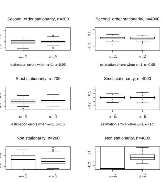
without the strict stationarity condition. A detailed discussion is provided in Section 7.3. Figure 4 presents some numerical evidence on the performance of the QMLE in finite samples through a simulation study. In all experi-ments, we use the sample sizen= 200and n= 4,000 with 100 replications. The data of the top panel are generated from the second-order stationary ARCH(1) model (1.1) with the true parameter θ0 = (1,0.95)′. The data of
the middle panel are generated from the strictly stationary ARCH(1) model withθ0 = (1,1.5)′ and infinite variance. In those two panels the results are
very similar, confirming that the second-order stationarity condition is not necessary for the use of the QMLE. The bottom panel, obtained for the ex-plosive ARCH(1) model with θ0 = (1,4)′, confirms the asymptotic results
for the QMLE ofα0. It also illustrates the impossibility of estimating the
pa-rameter ω0 with a reasonable accuracy under the nonstationarity condition
(1.5). The results concerningω0 even worsen when the sample size increases.
6.2. Finite sample properties of the tests.
6.2.1. On simulated data. To assess the performance of the tests devel-oped in Section3, we simulated N = 1,000 independent trajectories of size n= 100,n= 500 and n= 1,000 of an ARCH(1) model. We used different values ofα0 and a double Gamma distribution forηt, with shape parameter
k = 3 and scale parameter s= 1/2√3. The density of that distribution is f(η) = ηk−1/{2(k−1)!}e−|η|/s, where k and s are such that Eη2
0 = 1 and
such that the assumptions of Proposition 5.1 are satisfied with a standard GARCH(1,1) volatility.
The results concerning the test (3.2) on α0 are presented in Tables 1-2.
ω − ω^ α − α^
−0.5
0.5
estimation errors when ω=1, α=0.95
Second−order stationarity, n=200
ω − ω^ α − α^
−0.2
0.1
estimation errors when ω=1, α=0.95
Second−order stationarity, n=4000
ω − ω^ α − α^
−0.5
0.5
estimation errors when ω=1, α=1.5
Strict stationarity, n=200
ω − ω^ α − α^
−0.2
0.1
estimation errors when ω=1, α=1.5
Strict stationarity, n=4000
ω − ω^ α − α^
−0.5
0.5
estimation errors when ω=1, α=4
Non stationarity, n=200
ω − ω^ α − α^
−0.2
0.1
estimation errors when ω=1, α=4
Non stationarity, n=4000
Fig 4.Boxplots of estimation errors for the QMLE of the parametersω0andα0of
Table 1
Relative frequency of rejection (in %) for the test (3.2) of the null hypothesis
H0:α0≤1against H1:α0>1at the nominal level α= 5%when the errors
follow a double Gamma distribution.
α0 0.8 0.9 0.95 1 1.1 1.2 1.3
n= 100 0.0 0.4 1.2 2.3 7.7 17.8 32.9
n= 500 0.0 0.2 0.8 2.4 22.8 66.9 90.8
n= 1,000 0.0 0.0 0.7 4.9 38.9 88.6 99.4
Table 2
As Table 1, but for testing the null hypothesisH0:α0≤3against H1:α0>3.
α0 2.8 2.9 2.95 3 3.1 3.2 3.3
n= 100 0.4 1.3 1.4 2.5 4.0 8.9 12.5
n= 500 0.1 0.5 1.9 3.5 10.0 28.5 47.9
n= 1,000 0.0 0.4 1.0 5.2 19.7 46.6 78.6
the test behaves similarly when the value tested corresponds to a stationary solution (Table1) or to a non stationary process (Table 2).
We now illustrate the behavior of the strict stationarity tests (3.10) and (3.11), through simulations of ARCH(1) models with values of α0
corre-sponding to γ0 < 0 (α0 ∈ {1.6,1.7,1.8}), γ0 = 0 (α0 = 1.895) and γ0 > 0
(α0 ∈ {2,2.1,2.2}). Tables3-4show that, as expected, the frequency of
rejec-tion of theCST-test increases withγ0 while, obviously, that of the CNS-test
decreases. The rejection frequencies of the two tests approach the nominal level whenγ0= 0 and nincreases.
Now consider testing strict stationarity in a GARCH(1,1) model using the tests developed for the ARCH(1). Tables 5-6 confirm the theoretical result of Section 5. More precisely, for n sufficiently large, the tests give the right conclusion when Γ < 0 and Γ > 0. Note that when Γ = 0 the rejection frequencies are far from the nominal 5% level corresponding to an ARCH(1). This is not surprising since, except in the ARCH(1) case, the
Table 3
Relative frequency of rejection of the stationarity hypothesisH0:γ0<0 of the
test (3.10) at the nominal level α= 5%in the ARCH(1) case. The parameter
α0= 1.895corresponds toγ0= 0.
α0 1.6 1.7 1.8 1.895 2 2.1 2.2
n= 100 0.2 1.4 2.9 6.4 11.8 21.3 33.8
n= 500 0.0 0.0 0.6 4.7 25.0 57.4 83.4
Table 4
As Table3, but for testing the nonstationarity hypothesis H0:γ0≥0 with the test (3.11). α0 1.6 1.7 1.8 1.895 2 2.1 2.2 n= 100 42.1 28.4 17.1 11.6 5.5 2.1 0.8 n= 500 90.0 61.4 23.8 6.7 0.9 0.0 0.0 n= 1,000 99.3 86.9 39.8 5.5 0.3 0.0 0.0 Table 5
As Table 3, but for standard GARCH(1,1) models withβ0= 0.8. The parameter α0= 0.226corresponds toΓ = 0.
α0 0.1 0.15 0.2 0.226 0.35 0.4 0.5
n= 100 0.0 0.0 0.0 0.0 0.0 0.0 0.6
n= 500 0.0 0.0 0.0 0.0 1.6 49.9 96.2
n= 1,000 0.0 0.0 0.0 0.0 55.1 96.0 99.8
asymptotic relative frequencies of rejection are unknown underΓ = 0. 6.2.2. On real data. The strict stationarity tests were then applied to the daily returns of 11 major stock market indices. We considered the CAC,
DAX, DJA, DJI, DJT, DJU, FTSE, Nasdaq,3 Nikkei, SMI and SP500, from
January 2, 1990, to January 22, 2009, except for the indices for which such historical data do not exist. Table7displays the test statisticsTncomputed
on each series. Note that, asn→ ∞, Tn=√n ˆ γn−γ0 ˆ σu +√nγ0 ˆ σu → −∞
in probability when γ0 < 0, and Tn → +∞ in probability when γ0 > 0.
Because the values of Tn given in Table 7 are very small, a nonstationary
augmented GARCH(1,1) model is not plausible, for any of these series.
3
Since the Nasdaq index level was halved on January 3, 1994, one outlier has been eliminated for this series.
Table 6
As Table 4, but for testing the nonstationarity hypothesisH0: Γ≥0 with the test (3.11).
α0 0.1 0.15 0.2 0.226 0.35 0.4 0.5
n= 100 100.0 100.0 98.5 95.3 26.6 10.7 2.9
n= 500 100.0 100.0 100.0 93.9 1.1 0.2 0.1
Table 7
Test statisticTn of the strict stationarity tests (3.10) and (3.11). The test
statistic is the realization of a random variable which is asymptotically N(0,1)
distributed when γ0= 0, tends to−∞under the strict stationarity hypothesis
γ0<0, tends to+∞whenγ0>0.
CAC DAX DJA DJI DJT DJU FTSE Nasdaq Nikkei SMI SP500
-86.1 -79 -80.8 -78.7 -87.2 -69.3 -75.3 -81.4 -86.7 -71.5 -80.8
7. Proofs and complementary results.
7.1. Asymptotic behaviors of (ht). As noted in the introduction, when
γ0 6= 0 the asymptotic behavior of the sequences(ht) (defined by (1.1)) and
(σt2)(defined by (1.4)) is the same and is easily obtained by the Cauchy rule. Whenγ0 = 0 the asymptotic behavior ofσ2t can be obtained by the
Chung-Fuchs theorem. The behavior of ht is different in this case and is described
in the result below.
Proposition 7.1. For the ARCH(1) model (1.1), the following proper-ties hold:
i) When γ0 >0, ht→ ∞ a.s. at an exponential rate:
for any ρ∈(e−γ0,1), ρth
t→ ∞ and ρtǫ2t → ∞ a.s. as t→ ∞.
ii) (Klüppelberg, Lindner and Maller (2004))
When γ0 = 0, ht→ ∞ and ǫ2t → ∞ in probability.
iii) Letψbe a decreasing bijection from(0,∞)to(0,∞) such thatEψ(ǫ21)<
∞. When γ0 = 0, (7.1) 1 n n X t=1 ψ(ǫ2t)→0 and 1 n n X t=1 ψ(ht)→0 in L1 as n→ ∞.
Proof.To provei)we note that
ht = ω0+α0ηt2−1ht−1 =ω0 ( 1 + t−1 X i=1 αi0η2t−1. . . η2t−i ) +αt0ηt2−1. . . η12ǫ20 ≥ ω0 t−1 Y i=1 α0ηi2, (7.2)
Thus, for any constant ρ∈(e−γ0,1),we have lim inf t→∞ 1 t logρ th t ≥ lim t→∞ 1 t ( logρω0+ t−1 X i=1 logρα0η2i ) = Elogρα0η12 = logρ+γ0>0.
It follows that logρth
t, and hence ρtht, tends to +∞ a.s as n → ∞.
For any real-valued function f, let f+(x) = max{f(x),0} and f−(x) = max{−f(x),0}, so that f(x) =f+(x)−f−(x). Since Elog+η12 ≤Eη21 = 1, we haveE|logη21| =∞ if and only if Elogη21 = −∞. Thus γ0 > 0 implies
E|logη2
1| < ∞, which entails that logηt2/t → 0 a.s. as t → ∞. Therefore,
lim inft→∞t−1logρtη2tht ≥ Elogρα0η12 > 0, and ρtǫ2t =ρtηt2ht → +∞ a.s.
by already given arguments.
The proof of ii) follows from Klüppelberg et al. (2004). Their condi-tion E
logλε21
< ∞ becomes in our notations E
logα0η21
< ∞, and this
condition is satisfied because E(logα0η21)+−E(logα0η12)− = γ0 = 0 and
E(logα0η21)+≤α0.
To prove iii) note that γ0 ≥ 0 implies α0 ≥ exp{−logEη12} = 1, by
Jensen’s inequality. Thus ht > ǫ2t−1 and ψ(ht) < ψ(ǫ2t−1). Therefore, the
second convergence in (7.1) will follow from first convergence. It suffices to consider the case ǫ0 = 0 and to show that Eψ(ǫt2) → 0ast → ∞. Note
that, even ifǫ2t does not increase with probability one,ǫ2t+1 is stochastically greater thanǫ2 t because ǫ2t+1 = (ω0+ω0α0η2t +· · ·+ω0αt0−1η2t· · ·η22+ω0αt0ηt2· · ·η12)ηt2+1 ≥ (ω0+ω0α0η2t +· · ·+ω0αt0ηt2· · ·η22)η2t+1 d = ǫ2t
where=d stands for equality in distribution. The dominated convergence the-orem andi)-ii)then entail
Eψ(ǫ2t) = Z ∞ 0 Pnǫ2t < ψ−1(u)odu→ Z ∞ 0 lim t→∞↓P n ǫ2t < ψ−1(u)odu= 0,
7.2. Asymptotic normality of the unrestricted QMLE ofα0.
Lemma 7.1. When γ0>0, we have
∞ X t=1 sup θ∈Θ ∂ ∂ωℓt(θ) < ∞ a.s., (7.3) ∞ X t=1 sup θ∈Θ ∂2 ∂ω∂θℓt(θ) < ∞ a.s., (7.4) sup θ∈Θ 1 n n X t=1 ∂2 ∂α2ℓt(ω, α0)− 1 α2 0 = o(1) a.s., (7.5) 1 n n X t=1 sup θ∈Θ ∂3 ∂α3ℓt(θ) = O(1) a.s., (7.6) When γ0 = 0, sup θ∈Θ 1 n n X t=1 ∂2 ∂α2ℓt(ω, α0)− 1 α2 0 = o(1) in probability, (7.7) 1 n n X t=1 sup θ∈Θ ∂3 ∂α3ℓt(θ) = O(1) in probability. (7.8)
Proof. Using Proposition 7.1, there exist a real random variable K and a constantρ∈(e−γ0,1),independent of θand t, such that
∂ ∂ωℓt(θ) = −(ω0+α0ǫ2t−1)η2t (ω+αǫ2 t−1)2 + 1 ω+αǫ2 t−1 ≤Kρt(ηt2+ 1). (7.9) Since P∞
t=1Kρt(η2t + 1) has a finite expectation, it is almost surely finite.
Thus (7.3) is proved, and (7.4) can be obtained by the same arguments. We have ∂2ℓt(ω, α0) ∂α2 − 1 α2 0 = ( 2(ω0+α0ǫ 2 t−1)ηt2 ω+α0ǫ2t−1 −1 ) ǫ4 t−1 (ω+α0ǫ2t−1)2 − 1 α2 0 = 2ηt2−1 ǫ 4 t−1 (ω+α0ǫ2t−1)2 − 1 α20 +r1,t = 2ηt2−1 1 α2 0 +r1,t+r2,t where sup θ∈Θ| r1,t|= sup θ∈Θ 2(ω0−ω)ηt2 (ω+α0ǫ2t−1) ǫ4t−1 (ω+α0ǫ2t−1)2 =o(1) a.s.
and sup θ∈Θ| r2,t| = sup θ∈Θ (2η2t −1) ( ǫ4 t−1 (ω+α0ǫ2t−1)2 − 1 α2 0 ) = sup θ∈Θ (2η2t −1) ( ω2+ 2α0ǫ2t−1 α2 0(ω+α0ǫ2t−1)2 ) =o(1) a.s. ast→ ∞. Therefore (7.5) is established. To prove (7.6), it suffices to remark that ∂3 ∂α3ℓt(θ) = ( 2−6(ω0+α0ǫ 2 t−1)ηt2 ω+αǫ2 t−1 ) ǫ2 t−1 ω+αǫ2 t−1 !3 ≤ 2 + 6 ω 0 ω + α0 α η2t 1 α3.
We obtain (7.7) and (7.8) similarly in view of Proposition 7.1iii).
Proof of Theorem2.1.i)andiv)have already been proven (see Berkes, Horváth and Kokoszka (2003) and Francq and Zakoïan (2004)).
To proveii)note that (ˆωn,αˆn) = arg minθ∈ΘQn(θ),where
Qn(θ) = 1 n n X t=1 {ℓt(θ)−ℓt(θ0)}. We have Qn(θ) = 1 n n X t=1 ηt2 ( σ2 t(θ0) σt2(θ) −1 ) + log σ 2 t(θ) σt2(θ0) = 1 n n X t=1 ηt2(ω0−ω) + (α0−α)ǫ 2 t−1 ω+αǫ2 t−1 + log ω+αǫ 2 t−1 ω0+α0ǫ2t−1 . For any θ∈Θ, we have α6= 0. Letting
On(α) = 1 n n X t=1 ηt2(α0−α) α + log α α0 and dt= α(ω0−ω)−ω(α0−α) α(ω+αǫ2 t−1) , we have, by Proposition 7.1, Qn(θ)−On(α) = 1 n n X t=1 η2tdt−1+ 1 n n X t=1 log (ω+αǫ 2 t−1)α0 (ω0+α0ǫ2t−1)α → 0 a.s.
Moreover this convergence is uniform on the compact setΘ:
(7.10) lim
n→∞supθ∈Θ|Qn(θ)−On(α)|= 0 a.s.
Let α−0 and α+0 denote two constants such that 0 < α−0 < α0 < α+0.
Intro-ducingσˆ2 η =n−1 Pn t=1η2t, the solution of α∗n= arg min α On(α)
isα∗n=α0ˆσ2η.This solution belongs to the interval(α−0, α+0) for sufficiently
largen. Thus (7.11) α∗∗n = arg min α6∈(α−0,α0+)On(α)∈ {α − 0, α+0} and (7.12) lim n→∞On(α ∗∗ n ) = min n lim n→∞On(α − 0),nlim→∞On(α+0) o >0. This result and (7.10) show that almost surely
lim
n→∞θ∈Θ, αmin6∈(α−
0,α+0)
Qn(θ)>0.
SinceminθQn(θ)≤Qn(θ0) = 0, it follows that
lim
n→∞arg minθ∈ΘQn(θ)∈(0,∞)×(α
−
0, α+0).
Because the interval(α−0, α+0) containingα0 can be chosen arbitrarily small,
ii)is proven.
Turning to the proof of iii) we first note that Proposition 7.1 entails n−1Pn
t=1Esupθ∈Θ|dt−1| → 0, which implies n1Ptn=1supθ∈Θηt2dt−1 → 0 in
L1. Using the elementary inequality |log(x/y)| ≤ |x−y|/x+|x−y|/y for x, y >0, Proposition7.1 also entails
n−1 n X t=1 log (ω+αǫ 2 t−1)α0 (ω0+α0ǫ2t−1)α →0
inL1 uniformly in θ. It follows that (7.10) can be replaced by
(7.13) lim
We now note that the asymptotic behavoir ofOn(α) is not affected by the
assumption onγ0. Thus (7.11) and (7.12) still hold. For allε >0, we clearly
have P ( min θ∈Θ, α6∈(α−0,α+0) Qn(θ)≤ε ) ≤ P ( min θ∈Θ, α6∈(α−0,α+0) On(θ)≤2ε ) +P ( sup θ∈Θ| Qn(θ)−On(α)|> ε ) . By (7.11)-(7.12), the first term of the right-hand side of the last inequality tends to zero when ε < limn→∞On(α∗∗n). The second term tends to zero
by (7.13) and the Markov inequality. Because Qn(ˆθn) ≤ Qn(θ0) = 0, we
conclude thatPnαˆn∈(α−0, α+0)
o
→1, which shows the weak consistency in
iii).
It remains to prove the asymptotic normality ofαˆn when γ0 >0. Notice
that we cannot use the fact that the derivative of the criterion cancels at ˆ
θn= (ˆωn,αˆn)since we have no consistency result forωˆn. Thus the minimum
could lie on the boundary of Θ, even asymptotically. However, the partial derivative with respect toαis asymptotically equal to zero at the minimum sinceαˆn→α0 and(ω0, α0)belongs to the interior ofΘ. Hence, an expansion
of the criterion derivative gives
1 √ n Pn t=1 ∂ω∂ ℓt(ˆθn) 0 ! = √1 n n X t=1 ∂ ∂θℓt(θ0) +Jn √ n(ˆθn−θ0) (7.14)
where Jn is a2×2matrix whose elements have the form
Jn(i, j) = 1 n n X t=1 ∂2 ∂θj∂θj ℓt(θ∗i)
where θi∗ = (ω∗i, α∗i) is between θˆn and θ0. By Proposition 7.1 i) and from
the central limit theorem we have 1 √ n n X t=1 ∂ ∂αℓt(θ0) = 1 √ n n X t=1 (1−ηt2) ǫ 2 t−1 ω0+α0ǫ2t−1 = √1 n n X t=1 (1−ηt2) 1 α0 +oP(1) d → N 0,κη −1 α2 0 . (7.15)
By (7.4) in Lemma 7.1and the compactness of Θ, we have (7.16) Jn(2,1)√n(ˆωn−ω0)≤ ∞ X t=1 sup θ∈Θ ∂2 ∂ω∂θℓt(θ) 1 √ n(ˆωn−ω0)→0 a.s. An expansion of the function
α7→ 1 n n X t=1 ∂2 ∂α2ℓt(ω∗2, α) gives Jn(2,2) = 1 n n X t=1 ∂2 ∂α2ℓt(ω∗2, α0) + 1 n n X t=1 ∂3 ∂α3ℓt(ω2∗, α∗)(α∗2−α0)
where α∗ is between α∗2 and α0. Using (7.5), (7.6) and ii)we get
(7.17) Jn(2,2)→
1 α20 a.s.
The conclusion follows, by considering the second component in (7.14) and
from (7.15), (7.16) and (7.17).
Proof of Theorem2.2.The proof of the asymptotic normality still relies on the Taylor expansion (7.14). By the Lindeberg central limit theorem for martingale differences (see Billingsley, 1995, p. 476), the asymptotic normal-ity (7.15) of the score vector is obtained by showing that
Var √1 n n X t=1 (1−ηt2) ǫ 2 t−1 ω0+α0ǫ2t−1 ! = κη−1 n n X t=1 E ǫ2t−1 ω0+α0ǫ2t−1 2 → (κη−1)α−02,
which is a consequence of Proposition 7.1 iii), and by noting that for all ε >0 κη −1 n n X t=1 E ǫ2t−1 ω0+α0ǫ2t−1 2 1 1−η2 t √ n ǫ2 t−1 ω0+α0ǫ2 t−1 >ε ≤ κη −1 α20 P |1−ηt2|> α0ε√n →0.
To deal with the second term in the right-hand side of (7.14) we cannot use (7.16) because (7.4) requires γ0 > 0. Instead, noting that σt2(θ∗2)/σ2t(θ0) is
bounded, we use |Jn(2,1)√n(ˆωn−ω0)| ≤ K √ n n X t=1 2η2 tσ2t(θ0) σ2 t(θ2∗) + 1 ! ǫ2t−1 σ4 t(θ∗2) ≤ √K n n X t=1 ηt2+ 1 ǫ 2 t−1 σ4 t(θ2∗) ,
where K >0 is a generic constant whose value can change along the proof. Hence, E|Jn(2,1)√n(ˆωn−ω0)| ≤ √K n n X t=1 E ǫ 2 t−1 (ω∗ 2+α∗2ǫ2t−1)2 ≤ √K n n X t=1 E 1 σ2 t−1(θ0) . Moreover, σ2t(θ0) =ω0(1 +Zt−1+Zt−1Zt−2+· · ·+Zt−1. . . Z1) +Zt−1. . . Z0σ20.
By AssumptionA, it follows that
(7.18) E|Jn(2,1)√n(ˆωn−ω0)| →0asn→ ∞. Finally, similarly to (7.17) (7.19) Jn(2,2)→ 1 α2 0 in probability
using iii) in Theorem 2.1, (7.7) and (7.8). The conclusion follows as in the
caseγ0>0.
Proof of Theorem 2.3. The convergence results in i) can be shown in a standard way, using Taylor expansions of the functions ˆκη =κη(ˆθn) and
ˆ
µn(p, q) = µn(p, q)(ˆθn) around θ0, and the ergodic theorem together with
the consistency ofθˆn.
Now consider the caseii). For some θ∗ = (ω∗, α∗)′ between θˆn and θ0 we
have (7.20) κˆη = 1 n n X t=1 η4t−2 n n X t=1 ǫ4t σt4(θ∗) 1 σ2t(θ∗) ∂σ2t(θ∗) ∂θ′ (θ∗−θ0) := 1 n n X t=1 ηt4+Rn.
By Proposition 7.1, for some constantsK >0 andρ∈(0,1),
|Rn| ≤ K n n X t=1 ηt4ρt|ω∗−ω0|+|α∗−α0| =oP(1)
where the last equality follows from the strong consistency of αˆn and the
fact that|ω∗−ω0|is bounded by compactness of Θ. Hence the first part of
ii)is proven. Now note that ˆ µn(2,2) = 1 ˆ α2 n + 1 n n X t=1 ( ǫ4 t ˆ ωn+ ˆαnǫ2t 2 − 1 ˆ α2 n ) = 1 ˆ α2 n− ˆ ωn2 ˆ α2 n ˆ µn(0,2)−2ωˆn ˆ αn ˆ µn(1,2). Similarly we have ˆ µn(1,2) =− ˆ ωn ˆ αn ˆ µn(0,2) + 1 ˆ αn ˆ µn(0,1). It follows that (7.21) ξˆn= ˆα2n ( 1−µˆ 2 n(0,1) ˆ µn(0,2) )−1 .
In order to show that ξˆn → α20, it thus remains to show that
ˆ
µ2n(0,1)/µˆn(0,2) =o(1)a.s. First note thatµˆn(0,2)≥n−1ωˆ−n2. Since
σt2(ˆθn) = ˆωn+ ˆαnηt2−1σt2−1(θ0)≥ω0αˆnαt0−2ηt2−1ηt2−2· · ·η12, we have nµˆn(0,1) = n X t=1 1 σ2 t+1(ˆθn) ≤ α0 ω0αˆn ∞ X t=1 1 αt 0η2tη2t−1· · ·η21 . By the Cauchy root test, the last series is almost surely finite because
lim sup t→∞ 1 αt 0ηt2ηt2−1· · ·η12 !1/t = exp(−γ0)<1 a.s.
We thus have shown thatµˆ2n(0,1) =O(n−1)a.s., which completes the proof ofii).
Turning toiii), we note that in (7.20),Rn=:Sn(θ∗−θ0) with
E|Sn| ≤ K n n X t=1 E 1 α∗ǫ2 t−1 (1, ǫ2t−1) ! →(0, K)
by Proposition 7.1iii).Since the first component of θ∗−θ0 is bounded, by
Theorem2.1iii), the first convergence is established. To complete the proof we note thatµˆn(0,2)≥Kn−1 and that, in view of AssumptionA,
E√n|µˆn(0,1)|= 1 √ n n X t=1 E 1 σt2+1(ˆθn) =o(1).
The conclusion follows from (7.21).
7.3. Inconsistency of ωˆn when γ0 ≥0. The previous results do not give
any insight on the asymptotic behavior of the QMLE of ω0. Similarly to
(7.15) it can be shown that the score vector satisfies
(7.22) √1 n n X t=1 ∂ ∂θℓt(θ0) d → N ( 0,(κη−1) 0 0 0 α−02 !) .
The form of the asymptotic variance shows that, for n sufficiently large and almost surely, the variation of the log-likelihood n−1/2Pnt=1logℓt(θ) is
negligible whenθ varies between (ω0, α0) and(ω0+h, α0) for small h.
Note that a score vector with a degenerate asymptotic varianceJcan arise when a central limit theorem with a non standard rate of convergence ap-plies. This is for instance the case in regressions with trends, or in unit root and cointegration models. In such situations, the rate of convergence of the QMLE is obtained by finding a diagonal matrix Λn such that the
asymp-totic distribution of ΛnPnt=1 ∂θ∂ℓt(θ0) is not degenerated. If, for instance,
Λn=diag(n−1, n−1/2) then the second component of QMLE is expected to
converge at the standard rate √n, and the first one at the faster rate n. The situation here is completely different. In the proof of Theorem 2.1it is shown that ∂ω∂ ℓt(θ0) =OP(ρt)with |ρ|<1 (see Equation (7.9) below). The
equation (7.22) can thus be extended as Λn n X t=1 ∂ ∂θℓt(θ0) d → N ( 0,(κη −1) 0 0 0 α−02 !) , Λn= λn 0 0 n−1/2 !
for any sequence λn tending to zero as n → ∞. It means that the
log-likelihood is completely flat in the direction whereα0 is fixed andω0 varies.
Thus there is little hope concerning the existence of any consistent estimator of ω0. This is in accordance with the numerical illustrations provided in
Section 6.
7.4. A constrained QMLE ofα0. The asymptotic behaviour of the QMLE
ˆ
αn being independent of ω0 whenγ0 >0, and the QMLE of ω0 being
estimating ω0. To this aim a constrained QMLE of α0, in which the first
component of θ is fixed to an arbitrary value ω, can be introduced. The estimator (7.23) αˆcn(ω) = arg min α∈Θ1 1 n n X t=1 ℓt(ω, α), Θ1 compact ⊂(0,∞)
was studied by Jensen and Rahbek (2004a). They proved that, whenγ0 >0,
(2.3) continues to hold when the QMLE αˆn is replaced by the constrained
QMLEαˆcn(ω0).4 In the appendix we prove that:
under the assumptions of Theorem 2.2, in particular γ0 = 0,
(7.24) √n(ˆαcn(ω)−α0)→ Nd
n
0,(κη−1)α20
o
, asn→ ∞. However, the next result shows that the restricted QMLE ofα0 is generally
inconsistent in the stationary case.
Proposition 7.2. Let (ǫt) be a stationary solution of the ARCH(1)
model with parametersω0 andα0, such that Eǫt4 <∞. Then, if ω 6=ω0
(7.25) αˆcn(ω) does not converge in probability to α0.
On the contrary, Theorems2.1-2.2 show that
(7.26) the QMLE of α0 is always CAN
(underA whenγ0= 0).
Proof of (7.24). First note that, by the arguments used to prove iii)in Theorem2.1, we have
(7.27) αˆcn(ω)→α0 in probability as n→ ∞.
A Taylor expansion of the criterion derivative gives 0 = √1 n n X t=1 ∂ ∂αℓt(ω,αˆ c n(ω)) = √1 n n X t=1 ∂ ∂θℓt(ω, α0) + 1 n n X t=1 ∂2 ∂α2ℓt(ω, α∗) ! √ n(ˆθn−θ0) (7.28) 4
In fact, the result was announced under the assumptionγ0≥0but their proof is only
valid underγ0>0because the a.s. convergence ofǫ2t to infinity is used (see their Lemma 1).
whereα∗is betweenαˆcn(ω)and α0. Another Taylor expansion yields, forα∗∗ betweenαˆc n(ω) and α0 1 n n X t=1 ∂2 ∂α2ℓt(ω, α0)− 1 n n X t=1 ∂2 ∂α2ℓt(ω, α∗) ≤ |α∗−α0| 1 n n X t=1 ∂2 ∂α3ℓt(ω, α∗∗) ≤ |α∗−α0| 1 n n X t=1 sup θ∈Θ ∂3 ∂α3ℓt(θ) = o(1) in probability,
using (7.27) and (7.8). Therefore, using (7.7), the term in parentheses in (7.28) converges to1/α2
0.To conclude, it remains to prove that
1 √ n n X t=1 ∂ ∂αℓt(ω, α0) d → N 0,κη−1 α2 0 . (7.29) We have 1 √ n n X t=1 ∂ ∂αℓt(ω, α0) = √1 n n X t=1 (1−η2t) ǫ 2 t−1 ω+α0ǫ2t−1 +√1 n n X t=1 ηt2 (ω−ω0)ǫ 2 t−1 (ω+α0ǫ2t−1)2 .
The last term tends to zero in probability, usingA, similarly to (7.18). The first term converges in distribution to the normal law of (7.29) by exactly
the same arguments as in the proof of Theorem2.2.
Proof of Proposition 7.2. The ergodic theorem entails that, almost surely, Ln(α) = 1 n n X t=1 ǫ2t σ2 t(ω, α) + logσt2(ω, α) → L(α) =E ( ω0+α0ǫ2t−1 ω+αǫ2 t−1 + logω+αǫ2t−1 )
asn→ ∞. The dominated convergence theorem implies that L′(α) =E ∂ ∂α ( ω0+α0ǫ2t−1 ω+αǫ2 t−1 + logω+αǫ2t−1 ) =E ( ǫ2t−1 ω+αǫ2t−12{(ω−ω0) + (α−α0)ǫ 2 t−1} ) .
First suppose that ω < ω0. Then L′(α) < 0 for α ≤ α0. The intermediate
values theorem shows that the functionL(·)has a minimum at a pointα∗ > α0 and thatL(α∗) < L(α0). Now suppose that ω > ω0. ThenL′(α) >0 for
α ≥α0. This shows that L(·) has a minimum at a point α∗ ∈ [0, α0), with
L(α∗)< L(α0). Thus, we have shown that for any ω6=ω0,the functionL(·) has a minimum at a pointα∗ 6=α0 and L(α∗)< L(α0).
A Taylor expansion ofLn(·) yields
(7.30) Ln{αˆcn(ω)}=Ln(α0) +L′n(˜αn){αˆcn(ω)−α0}
whereα˜nis betweenαˆcn(ω)andα0. Note that sinceEǫ4t <∞, almost surely,
lim sup n→∞ supα L′n(α) ≤ lim n→∞ 1 n n X t=1 1 + ǫ 2 t ω ! ǫ2t−1 ω <∞. Now suppose that
(7.31) αˆcn(ω)→α0, in probability asn→ ∞.
Then, it follows from (7.30) that
Ln{αˆcn(ω)} →L(α0), in probability asn→ ∞.
Then, taking the limit in probability in the following inequality Ln{αˆcn(ω)} ≤Ln(α∗)
we find thatL(α0)≤L(α∗),which is in contradiction with the definition of
α∗ 6=α0. Thus (7.31) cannot be true.
7.5. Stationarity test. Proof of Theorem 3.1. First consider the case γ0 < 0. Let ζn = n−1Pnt=1logη2t. Note that ζˆn = ζn(ˆθn) and ζn = ζn(θ0)
with ζn(θ) = n−1Pnt=1logη2t(θ) and ηt(θ) = ǫt/σt(θ). A Taylor expansion
thus gives (7.32) ζˆn=ζn+ ∂ζn(θ0) ∂θ′ (ˆθn−θ0) +oP(n− 1/2) with ∂ζn(θ0) ∂θ′ = −1 n n X t=1 1 ht ∂σ2 t(θ0) ∂θ′ . Moreover the QMLE satisfies
(7.33) √n(ˆθn−θ0) =−J−1 1 √ n n X t=1 vt 1 ht ∂σ2t(θ0) ∂θ +oP(1).
In view of (7.32) and (7.33), we have √ n(ˆζn−ζ) = 1 √ n n X t=1 ut+ Ω′J−1 1 √ n n X t=1 vt 1 ht ∂σ2 t(θ0) ∂θ +oP(1), where Ω =Eh−t1∂σ2 t(θ0)/∂θ. Note that Cov √1 n n X t=1 ut, Ω′J−1 1 √ n n X t=1 vt 1 ht ∂σ2t(θ0) ∂θ ! = σuvΩ′J−1Ω.
The Slutsky lemma and the central limit theorem for martingale differences thus entail √ n ˆζˆn−ζ θn−θ0 ! d → N ( 0,Σ := σ 2 u+ (σv2+ 2σuv)Ω′J−1Ω −(σv2+σuv)Ω′J−1 −(σv2+σuv)J−1Ω σv2J−1 !) . Noting thatθ′
0∂σt2(θ0)/∂θ=ht almost surely, we have
E ( 1 ht ∂σ2t(θ0) ∂θ 1− 1 ht ∂σt2(θ0) ∂θ′ θ0 !) = 0,
which entailsJθ0 = Ω. Thus J−1Ω =θ0 and Ω′J−1Ω = 1, and (3.5) follows.
The convergence in probability in (3.6) is a straightforward consequence of (3.5). By direct application of the delta method (seee.g. Theorem 3.1 in van der Vaart, 1998), in the caseγ0 <0
√
n(ˆγn−γ0)→ Nd 0, LΣL′ where L=
1,0, α−01.
It is easy to verify thatLΣL′ =σu2+σ2vnαξ2 0 −1
o
. Now consider the case γ0 ≥0. Note that,
∂2ζn(θ) ∂θ∂θ′ =Jn(θ) := 1 n n X t=1 1 σ4 t(θ) ∂σ2t(θ) ∂θ ∂σ2t(θ) ∂θ′ →J(θ) := 0 0 0 α−2 !
a.s. (resp. in probability) as n → ∞ when γ0 > 0 (resp. when γ0 = 0),
uniformly in θ ∈ Θ, by Proposition 7.1. Moreover the matrix ΛnJn(θ)Λn
converges to the same limit, where Λn is the diagonal matrix with elements
n1/4 and 1. Thus (7.34) ζˆn=ζn+ ∂ζn(θ0) ∂θ′ (ˆθn−θ0)+ 1 2(ˆθn−θ0) ′Λ−1 n ΛnJn(θ∗)ΛnΛn−1(ˆθn−θ0).
Noting that Λ−n1(ˆθn −θ0) tends to zero (a.s. when γ0 > 0, in probability
whenγ0= 0), we conclude that (7.32) still holds. By the same arguments,
1 n n X t=1 1 ht ∂σ2t(θ0) ∂θ′ → 0 α−01 !
a.s. (in probability when γ0 = 0).
Therefore (7.35) √n(ˆζn−ζ) = 1 √ n n X t=1 ut−α−01 √ n( ˆαn−α0) +oP(1).
From the proof of (2.3) and Theorem 2.2, it can be seen that (7.36) √n(ˆαn−α0) =−α0n−1/2
n X t=1
vt+oP(1),
and (3.8) follows. The rest of the proof is as in the case γ0<0.
Proof of Corollary 3.2. By arguments used in the proof of Theorem2.3, ˆ
σu2 converges almost surely to σu2 when γ < 0 or γ ≥ 0. Therefore Tn =
√
n(ˆγn−γ0)/σˆu+√nγ0/σˆu converges in probability to−∞ whenγ <0, to
+∞ when γ >0, and in distribution to theN(0,1) whenγ0= 0.
Proof of Proposition 4.1. We consider the caseγ0≥0 because the LAN
of GARCH models has already be established in the stationary case (see Drost and Klaassen (1997), Lee and Taniguchi (2005)). A Taylor expansion ofτn7→Λn,f(θ0+τn/√n, θ0)around0 yields (7.37) Λn,f(θ0+τn/√n, θ0) =τn′Sn,f(θ0)− 1 2τn′In(θ∗n)τn, where θ∗ n=θ0+τn∗/ √ n withτ∗ n between 0 andτn, (7.38) Sn,f(θ0) = − 1 √ n n X t=1 1 +ηt f′(ηt) f(ηt) 1 2σ2t(θ0) ∂σt2(θ0) ∂θ
and, introducing the functiong(y) = 1 + 2y(f′/f)(y) +y2(f′/f)′(y),
In(θ) =−(1/4n) n X t=1 g ǫ t σt(θ) ∆t(θ), ∆t(θ) = 1 σt4(θ) ∂σ2 t(θ) ∂θ ∂σ2 t(θ) ∂θ′ . As in the proof of Theorem 2.2, the Lindeberg central limit theorem for martingale differences shows that
Let the matrix norm defined bykAk=P
|aij|with standard notations. We
have k∆t(θ)−∆t(θ0)k ≤ |ω0−ω| 2 ωω0 + 1 αω0 + 1 α0ω +|α0−α| 2 αα0 + 1 αω0 + 1 α0ω = O(kθ−θ0k).
Note that (4.2)-(4.3) implies E|g(η1)|<∞. The law of large numbers then
entails lim n→∞ 1 n n X t=1 g(ηt){∆t(θ)−∆t(θ0)} ≤ O(kθ−θ0k) lim n→∞ 1 n n X t=1 |g(ηt)|=O(kθ−θ0k) a.s. and lim n→∞ 1 n n X t=1 g(ηt){∆t(θn∗)−∆t(θ0)} = 0 a.s. Noting that ǫt σt(θ) = σt(θ0) σt(θ) ηt ≤ rω 0 ω + rα 0 α |ηt|,
and thatsupθk∆t(θ)k=O(1), Assumption (4.2) and the mean value
theo-rem entail 1 n n X t=1 g ǫ t σt(θ) −g(ηt) ∆t(θ) ≤O(kθ−θ0k) 1 n n X t=1 |ηt|δ+1.
The Hölder inequality shows thatE|ηt|δ+1 ≤ q
E|ηt|2δEη2t, which is finite
under (4.3). It follows that 1 n n X t=1 g ǫ t σt(θn∗) −g(ηt) ∆t(θn∗) →0 a.s.
We thus have shown that, asn→ ∞,
(7.40) kIn(θ∗
n)−In(θ0)k →0 a.s.
Integrations by parts show that, under (4.1), we have R
y2f′′(y)dy =
−2R
that E 1 n n X t=1 g(ηt) ( ∆t(θ0)− 1/α0 0 !) ≤ E|g(η1)|E 1 n n X t=1 1 ω0+α0ǫ2t−1 ω0 ω0+α0ǫ2t−1 →0, and thus, by the law of large numbers
(7.41) In(θ0) = 1 n n X t=1 −g(ηt) 4 0 1/α0 ! +OPθ0(1)→If in probability as n→ ∞.
The conclusion follows from (7.37)–(7.41).
Proof of Proposition 4.2. For simplicity, writeP instead of Pn,0. By the
delta method and (7.36) we obtain
√ n(log ˆαn−logα0) = 1 α0 √ n( ˆαn−α0) +oP(1) =− 1 √ n n X t=1 vt+oP(1).
In view of (7.35), and noting ζ+ logα0= 0, we have
Tn=√n ˆ ζn−ζ+ log ˆαn−logα0 ˆ σu = √1 n n X t=1 ut σu +oP(1).
By (4.4) and (7.38), it follows that underP
(7.42) Tn Λn,f(θ0+τ /√n, θ0) ! d −→ N 0 −τ22ιf 8α2 0 , 1 c c τ22ιf 4α2 0 , where (7.43) c=− τ2 2α0σu Eu1 1 +η1 f′(η1) f(η1) = τ2 α0σu .
For the last equality, we used an integration by parts and we noted that Eη21 <∞ entails limx→±∞xlogx2f(x) = 0. Le Cam’s third lemma (see e.g. van der Vaart, 1998, page 90) shows that
Tn−→ Nd τ 2 α0σu ,1 , under Pn,τ.
The conclusion easily follows.
Proof of Proposition 4.3. Distinguishing the cases γ0 < 0 and γ0 ≥ 0,
and reasoning as in the proof of Proposition4.2, it can be shown thatαˆn is
a regular estimator ofα∗, in the sense that
√ n(ˆαn−α∗−τ2/√n) q (ˆκη−1)ˆξn d → N (0,1), under Pα∗ n,τ as n→ ∞.
The conclusion easily follows.
Proof of Proposition4.4.In view of (4.6) and (4.8), theCST-test is asymp-totically optimal if and only if τ2/α0σu = τ2/
q
4α2
0/ιf, which is equivalent
to σu2ιf = 4. In the second equality of (7.43), we have seen that
Z (logy2−ζ) 1 + f′(y) f(y)y f(y)dy = −2. Thus, the Cauchy-Schwarz inequality yields
4 ≤ Z (logy2−ζ)2f(y)dy Z 1 +f′(y) f(y)y 2 f(y)dy =σu2ιf
with equality iff there exists a 6= 0 such that 1 + ηtf′(ηt)/f(ηt) =
a logη2t −ζ
a.s. Such densities f must satisfy the differential equation f′(y)/f(y) = 2alog|y|/y−(1+ζa)/y for almost everyy. Settinga=−1/2σ2
and b=ζ/4σ2, the solutions are two-sided generalized log-normal densities
of the form
f(y) = 1
2σ√2πe2b2σ2e
−(log2σ|y2|)2|y|−1+2b, σ2 >0, b∈R.
Direct computations show that R
logy2f(y)dy = 4bσ2 and R
y2f(y)dy = exp{2σ2(2b+ 1)}, which shows that the test is optimal iff f is given by (4.11).
We now give the proof of the first result. In view of (4.7) and (4.9), the Cα∗-test is asymptotically optimal if and only if(κη−1)ιf = 4. By Corollary
1 in Francq and Zakoïan (2006b), the solutions of this equation are given by
(4.11).
Proof of Proposition 5.1. We start by considering the caseΓ>0.By the arguments given in the proof of Proposition7.1i),ht→ ∞ andǫ2t → ∞
a.s. at an exponential rate ast→ ∞. Let α∗0=E a(η t) η2t .
Following the lines of the proof of Theorem 2.1, note that (ˆωn,αˆn) =
arg minθ∈ΘQn(θ),where
Qn(θ) = 1 n n X t=1 ( ǫ2 t ω+αǫ2t−1 + log(ω+αǫ 2 t−1)− ǫ2 t α∗0ǫ2t−1 −log(α ∗ 0ǫ2t−1) ) . Letting On(α) = 1 n n X t=1 ηt2a(ηt−1) η2 t−1 (α∗0−α) αα∗ 0 + log α α∗ 0
we have (7.10) by arguments already used. Noting that arg min α On(α) = 1 n n X t=1 η2ta(ηt−1) η2 t−1 →α∗0, a.s.
we conclude, as in the proof of Proposition7.1ii), thatαˆn→α∗0, a.s.Note
that fort large enough ωs(η
t)/hst < ωs(ηt)/t, and limt→∞ωs(ηt)/t →0 a.s.
We thus have 1 n n X t=1 log ˆη2t = 1 n n X t=1 log ǫ 2 t ˆ αnǫ2t−1 +oP(1) = 1 n n X t=1 logη 2 t{ω(ηt−1) +a(ηt−1)ht−1} ˆ αnht−1η2t−1 +oP(1) → Γ−logα∗0,
and the first result follows. The convergence of σˆ2
u is obtained by similar
arguments. By assumption E|logη21|2 >0, which entails that η2
1 has a
non-degenerate distribution. It follows that the a.s. limit ofσˆu2 is positive. Now consider the case Γ< 0.Letting η∗2
t =ǫ2t/(ω∗+α∗ǫ2t−1), and using
the inequality|log(x∗/x)| ≤ |x∗−x|/min(x, x∗) for all x, x∗>0, we have
1 n n X t=1 logηˆt2/ηt∗2 ≤ 1 n n X t=1 ω∗−ωˆn+ (α∗−αˆn)ǫ2t−1 ω∗+α∗ǫ2 t−1 →0 a.s. with ω∗ > 0 and α∗ > 0. By the arguments used in Berkes, Horváth, and Kokoszka (2003, Lemma 2.3), we have E|ǫt|2s < ∞. Applying the ergodic
theorem to(logηt∗2), it follows that
Γ∗=Elogα∗ηt∗2 =Elogα∗ǫ2t/(ω∗+α∗ǫ2t−1)<0.
The convergence of ˆσ2u to a positive limit is obtained by arguments already
References
Aue A., and L. Horváth (2009) Quasi-likelihood Estimation in Station-ary and NonstationStation-ary Autoregressive Models With Random Coeffi-cients.Preprint
Berkes, I., Horváth, L. and P.S. Kokoszka (2003) GARCH processes: structure and estimation.Bernoulli 9, 201–227.
Billingsley P. (1995) Probability and Measure. John Wiley, New York.
Bollerslev, T. (1986) Generalized autoregressive conditional heteroskedas-ticity.J. Econometrics31, 307–327.
Drost, F. C. and C. A. J. Klaassen (1997) Efficient estimation in semi-parametric GARCH models.Journal of Econometrics 81, 193–221.
Drost, F.C., Klaassen, C.A.J. and B.J.M. Werker (1997) Adaptive estimation in time-series models.Annals of Statistics 25, 786–817.
Engle, R.F. (1982) Autoregressive conditional heteroskedasticity with es-timates of the variance of the United Kingdom inflation.Econometrica
50, 987–1007.
Francq, C. and J.M. Zakoïan (2004) Maximum Likelihood Estimation
of Pure GARCH and ARMA-GARCH Processes. Bernoulli 10, 605–
637.
Francq, C. and J-M. Zakoïan (2006a) Mixing properties of a general class of GARCH(1,1) models without moment assumptions on the ob-served process. Econometric Theory22, 815–834.
Francq, C. and J.M. Zakoïan (2006b) On efficient inference in GARCH processes.In: Bertail P, Doukhan P, Soulier P (eds) Statistics for de-pendent data. Springer, New-York: 305–327
Goldie, C.M. and R.A. Maller (2000) Stability of perpetuities. Annals of Probability28, 1195–1218.
Hörmann, S. (2008) Augmented GARCH sequences: dependence structure and asymptotics.Bernoulli14, 543–561.
Jensen, S.T. and A. Rahbek (2004a) Asymptotic normality of the
QMLE estimator of ARCH in the nonstationary case. Econometrica
72, 641–646.
Jensen, S.T. and A. Rahbek (2004b) Asymptotic inference for
nonsta-tionary GARCH.Econometric Theory 20, 1203–1226.
Klüppelberg, C., Lindner, A. and R. Maller (2004) A continuous time GARCH Process driven by a Lévy process: stationarity and second order behaviour. Journal of Applied Probability 41, 601–622.
Lee, S. and M. Taniguchi (2005) Asymptotic theory for ARCH-SM models: LAN and residual empirical processes. Statistica Sinica 15, 215–234.
Ling, S. and M. McAleer (2003) Adaptative estimation in nonstationary ARMA models with GARCH errors.The Annals of Statistics31, 642– 674.
Linton, O., Pan, J. and H. Wang (2009) Estimation for a non-stationary semi-strong GARCH(1,1) model with heavy-tailed errors. To appear inEconometric Theory.
Nelson, D.B. (1990) Stationarity and persistence in the GARCH(1,1) model.Econometric Theory 6, 318–334.
van der Vaart, A.W. (1998)Asymptotic statistics.Cambridge University Press, United Kingdom.
BP 60149
59653 Villeneuve d’Ascq cedex France
E-mail:[email protected]
15 Boulevard Gabriel Peri 92245 Malakoff Cedex France