Volume 14 | Issue 2 Article 3
11-1-2015
Vol. 14, No. 2 (Full Issue)
JMASM Editors
Follow this and additional works at:http://digitalcommons.wayne.edu/jmasm
Part of theApplied Statistics Commons,Social and Behavioral Sciences Commons, and the Statistical Theory Commons
Recommended Citation
Editors, JMASM (2015) "Vol. 14, No. 2 (Full Issue),"Journal of Modern Applied Statistical Methods: Vol. 14 : Iss. 2 , Article 3. DOI: 10.22237/jmasm/1446350520
Journal of
Modern Applied
Statistical Methods
Shlomo S. Sawilowsky SENIOR EDITOR College of Education Wayne State UniversityHarvey Keselman ASSOCIATE EDITOR EMERITUS
Department of Psychology University of Manitoba
Jack Sawilowsky EDITOR
Reason Statistical Consulting
Alan Klockars
ASSISTANT EDITOR EMERITUS
Educational Psychology University of Washington
Bruno D. Zumbo ASSOCIATE EDITOR
Measurement, Evaluation, & Research Methodology University of British Columbia
Vance W. Berger ASSISTANT EDITOR
Biometry Research Group National Cancer Institute
Todd C. Headrick ASSISTANT EDITOR
Educational Psychology & Special Education So. Illinois University−
Carbondale
Joshua Neds-Fox EDITORIAL ASSISTANCE
Heather Marie Perrone EDITORIAL ASSISTANCE
JMASM (ISSN 1538−9472, http://digitalcommons.wayne.edu/jmasm) is an independent, open access electronic journal, published biannually in May and November by JMASM Inc. (PO Box 48023, Oak Park, MI, 48237) in collaboration with the Wayne State University Library System. JMASM seeks to publish (1) new statistical tests or procedures, or the comparison of existing statistical tests or procedures, using computer-intensive Monte Carlo, bootstrap, jackknife, or resampling methods, (2) the study of nonparametric, robust, permutation, exact, and approximate randomization methods, and (3) applications of computer programming, preferably in Fortran (all other programming environments are welcome), related to statistical algorithms, pseudo- random number generators, simulation techniques, and self-contained executable code to carry out new or interesting statistical methods.
Journal correspondence (other than manuscript submissions) and requests for advertising may be forwarded to
Journal of Modern Applied Statistical Methods
Vol. 14, No. 2
November 2015
Table of Contents
Invited Articles
2 – 8 R. WILCOX Inferences About the Skipped Correlation Coefficient: Dealing with Heteroscedasticity And Non-Normality
9 – 26 D. W. ZIMMERMAN Resolving the Issue of How Reliability B. D. ZUMBO Is Related to Statistical Power:
Adhering to Mathematical Definitions 27 – 34 T. R. KNAPP In (Partial) Defense of .05
Regular Articles
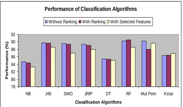
35 – 52 I. SANGAIAH An Empirical Study on Different Ranking A. V. A. KUMAR Methods for Effective Data Classification A. BALAMURUGAN
53 – 67 A. F. LUKMAN Two Stage Robust Ridge Method in a Linear O. I. OSOWOLE Regression Model
K. AYINDE
68 – 87 K. A. ADELEKE Semi-Parametric Non-Proportional Hazard A. A. ABIODUN Model with Time Varying Covariate R. A. IPINYOMI
88 – 109 A. I. AL-OMARI New Entropy Estimators with Smaller Root Mean Squared Error 110 – 122 G. PRAKASH Bayesian Analysis Under Progressively
123 – 140 D. AYDIN Monte Carlo Comparison of the Parameter B. ŞENOĞLU Estimation Methods for the Two-Parameter
Gumbel Distribution 141 – 158 K. AHMAD Structural Properties of
S. P. AHMAD Transmuted Weibull Distribution A. AHMED
159 – 171 N. S. M. SHARIFF A Robust Panel Unit Root Test
N. A. HAMZAH In the Presence of Cross Sectional Dependence 172 – 200 B. F. AJIBADE The Distribution of the Inverse Square Root
C. R. NWOSU Transformed Error Component of the J. I. MBEGBU Multiplicative Time Series Model
201 – 218 T. LEE The Bayes Factor for Case-Control Studies With Misclassified Data
219 – 235 Y. WOOLURU Approaches for Detection of Unstable Processes: D. R. SWAMY. A Comparative Study
P. NAGESH
236 – 256 D. S. BARRON Contrails: Causal Interference J. H. BROWN Using Propensity Scores
257 – 274 T. TIKHOMIROVA Statistical Modeling of Migration Attractiveness Y. LEBEDEVA Of the EU Member States
Statistical Software Applications and Review
275 – 281 A. J. LORENZ Caution for Software Use B. S. MARKMAN Of New Statistical Methods (R) S. S. SAWILOWSKY
Algorithms and Code
282 – 292 D. A. WALKER Two Group Program for Cohen's d, Hedges’ g,
η2, R
Dr. Wilcox is Professor of Psychology at the University of Southern California. Email him at [email protected].
Invited Article
Inferences About the Skipped Correlation
Coefficient: Dealing with Heteroscedasticity
and Non-Normality
Rand Wilcox
University of Southern California Los Angeles, CA
A common goal is testing the hypothesis that Pearson’s correlation is zero and typically this is done based on Student’s T test. There are, however, several well- known concerns. First, Student’s T is sensitive to heteroscedasticity. That is, when it rejects, it is reasonable to conclude that there is dependence, but in terms of making a decision about the strength of the association, it is unsatisfactory. Second, Pearson’s correlation is not robust: it can poorly reflect the strength of the association. Even a single outlier can have a tremendous impact on the usual estimate of Pearson’s correlation, which can result in a poor indication of the strength of the association among the bulk of the points. Numerous robust correlation coefficients have been proposed that deal with outliers among the marginal distributions, but these methods do not take into account the overall structure of the data in terms of dealing with outliers. A skipped correlation addresses this concern and methods for testing the hypothesis that this correlation is zero have been studied. However, there are serious limitations associated with one of these methods and extant studies regarding an alternative percentile bootstrap method do not address practical concerns reviewed in the paper. A minor goal is to report situations where this percentile bootstrap method can be unsatisfactory. The main result is that an alternative percentile bootstrap method performs well in simulations.
Keywords: Robust measures of association, level robust methods, non-normality, heteroscedasticity
Introduction
A basic goal is testing the hypothesis that the strength of the association between two random variables is zero. Certainly the best-known strategy is to test the hypothesis that Pearson’s correlation is zero, using Student’s T test.
0: 0
H (1)
There are, however, well known concerns with this approach. First, Student’s T assumes homoscedasticity. In practical terms, it provides a reasonable test of the hypothesis that two variables are independent, but in terms of making inferences about ρ, it can be unsatisfactory. For example, even when the null hypothesis is true, the probability of rejecting can increase as the sample size increases when there is heteroscedasticity (e.g., Wilcox, 2012). Roughly, the reason is that Student’s T uses the wrong standard error when there is heteroscedasticity, given the goal of testing (1).
Another concern is that r, the usual estimate of ρ, is not robust. Even a single outlier can result in a poor reflection of the strength of the association among the bulk of the points. Numerous robust estimators have been proposed for dealing with outliers among the marginal distributions (e.g., Wilcox, 2012, chapter 9). Certainly the two best-known approaches are Kendall’s tau and Spearman’s rho. But a known concern with these measures of association is that they do not deal with outliers in a manner that takes into account the overall structure of the data. That is, based on the random sample (X1, Y1), …, (Xn, Yn),
situations are encountered where no outliers are detected among X1, …, Xn,
ignoring Y, and no outliers are detected among Y1, …, Yn, ignoring X, yet there are
outliers that can have a substantial impact on Kendall’s tau, Spearman’s rho and other measures of association that do not deal with the overall structure of the data (e.g., Wilcox, 2012, chapter 9). A measure of the strength of an association that deals with this issue is the skipped correlation coefficient. The basic strategy is to use some outlier detection method that takes into account the overall structure of the data, remove any outliers that are found, and then compute Pearson’s correlation using the remaining data.
There are many outlier detection methods that take into account the overall structure of the data. In the context of a skipped correlation, a projection type outlier detection method has been the focus of attention. No single outlier detection method dominates, but the projection-type method used here appears to perform relatively well in terms of avoiding masking and detecting truly unusual points (e.g., Wilcox, 2012). Masking refers to missing outliers due to their very presence. For example, in the univariate case, detecting outliers using the mean and standard deviation can result in masking. The basic problem is that outliers inflate the sample standard deviation, which in turn can result is missing even extreme outliers.
Based on the projection type method for detecting outliers, let ξ denote the population analog of the skipped correlation and consider the goal of testing
0: 0
H (2)
A very simple approach is described in Wilcox (2012, Section 9.4.4). However, the method is limited to testing at the α = 0.05 level and it assumes homoscedasticity. More recently, Pernet, Wilcox and Rousselet (2013) studied a bootstrap method when sampling from a bivariate normal distribution. But the impact of non-normality and heteroscedasticity was not addressed. A minor goal in this paper is to report results indicating situations where the Pernet et al. method can be unsatisfactory when dealing with non-normality and heteroscedasticity. The primary goal is to report simulation results on an alternative bootstrap method that provides good control over the Type I error probability for a broader range of situations.
Description of the methods to be compared
This section describes the projection outlier detection method followed by the two percentile bootstrap methods that were studied when testing (2). For brevity, just an outline of the method is provided. Complete computational details can be found in Wilcox (2012, section 6.4.9). Included is an R function called outpro for applying it, which is used here.
The projection method begins by estimating the center of the data cloud, say ˆ
. Here this is done using the marginal medians. Then for fixed i, project all n
points onto the line connecting ˆ and (Xi, Yi). Based on the projected points, let
Dj (j = 1, …, n) be the distance between the projection of (Xj, Yj) and the center, ˆ. Next, check for outliers using the usual boxplot rule based on the Dj values. That is, if q1 and q2 are estimates of the lower and upper quartiles, respectively, based
on D1, …, Dn, declare Dj an outlier if Dj < 1.5(q2 − q1) or if Dj > 1.5(q2 − q1), in
which case (Xj, Yj) is declared an outlier as well. This process is performed for each i (i = 1, …, n) and (Xj, Yj) is declared an outlier if its projected distance is flagged as an outlier for any i.
The percentile bootstrap method used by Pernet et al. (2013) is applied as follows:
1. Remove any points flagged as outliers using the projection method. Let m denote the sample size after outliers are removed.
2. Generate a bootstrap sample from the remaining data by resampling with replacement m points.
3. Compute Pearson’s correlation based on this bootstrap sample yielding r*.
4. Repeat steps 2-3 and B times yielding r1∗, …, rB∗.
5. Put the values r1∗, …, rB∗ in ascending order and label the results
(1) ( )B
r r .
6. Let l = αB/2, rounded to the nearest integer and u = B − l. Then the 1 − α confidence interval for ξ is taken to be (r(l + 1), r(u)). This will be
called method B1 henceforth.
An unusual feature of method B1 is that the process of generating bootstrap samples does not exactly mimic the manner in which the data are generated and the skipped correlation is computed. A percentile bootstrap method that does mimic the way data are generated, labeled method B2 here, begins by generating a bootstrap sample from all n points, removing any points flagged as outliers and then computing ˆ*, Pearson’s correlation based on the remaining data. That is, in the description of method B1, replace steps 1-3 with
1. Generate a bootstrap sample by resampling with replacement n
points from the entire sample of size n.
2. Remove any points from the bootstrap sample in step 1 that are flagged as outliers using the projection method.
3. Compute Pearson’s correlation using the points not flagged as outliers in step 2.
As done in step 4 of method B1, this process is repeated B times only now the results are labeled
ˆ1*, ,
ˆB*. The 1 − α confidence interval for ξ is taken to be
* *
1 ˆ , ˆ u l
.It is noted that a p-value is readily computed when testing (2), which is motivated by general results in Liu and Singh (1997). Let Q* be the proportion of
*
ˆ
Simulation results
Four types of distributions are considered: normal, symmetric and heavy-tailed (roughly meaning that outliers tend to be common), asymmetric and relatively light-tailed, and asymmetric and relatively heavy-tailed. More specifically, g-and-h distributions (Hoaglin, 1985) are used, which arise as follows. Let Z be a random variable having a standard normal distribution and let
2
exp 1 exp / 2 gZ W hZ g If g = 0 2 exp 2 Z W Z h Then W has a g-and-h distribution, where g and h are parameters that determine the first four moments. The four distributions used here are the standard normal (g = h = 0), a symmetric heavy-tailed distribution (h = .2, g = 0), an asymmetric distribution with relatively light tails (h = 0, g = .2), and an asymmetric distribution with heavy tails (g = h = .2). Table 1 summarizes the skewness (γ1) and kurtosis (γ2) of these distributions.
The number of bootstrap samples was taken to be B = 1000. Bradley (1978) suggests that as a general guide, when testing at the .05 level, the actual level should be between .025 and .075. Preliminary simulations based on B = 500 indicated that method B2 does not satisfy this criterion; increasing B to 1000 gave more satisfactory results.
Table 1. Some properties of the g-and-h distribution.
g h κ2 κ1
0.0 0.0 0.00 3.00
0.0 0.2 0.00 21.46
0.2 0.0 0.61 3.68
0.2 0.2 2.81 155.98
Observations were generated according to the model Y = λ(X)ε, where both
heteroscedasticity. Three choices for λ(X) were used: λ(X) ≡ 1 (homosecdasticity),
λ(X) = |X| + 1 (so the conditional variance of Y, given X, is smallest when X is close to its mean), and λ(X) = 1/(|X| + 1) (in which case the conditional variance of
Y, given X, is largest when X is close to its mean. For convenience these three choices for λ will be called variance patterns (VP) 1, 2 and 3, respectively.
The simulation estimates of the actual Type I error probabilities were based on 2,000 replications. A common suggestion is that ideally, simulation estimates be based on 10,000 replications. However, when using method B2, a single replication takes a little over 14 seconds using the software R on a MacBook Pro with a 2.5 GHz processor. So 10,000 replications would require over 38 hours of execution time. To add perspective on the precision of the estimates, assuming Bradley’s criterion is reasonable, consider the issue of whether the actual level is less than or equal .075. Using the method in Pratt (1968), it can be seen that based on a two-sided .95 confidence interval for the actual level, the confidence interval will not contain .075 if ˆ ≤ .063. In a similar manner, based on a two-sided .95 confidence interval, the confidence interval for the actual level does not contain .025 if ˆ ≥ .0325.
Table 2. Estimated Type I error probabilities, n = 40, α = .05
g h VP B2 B1 0.0 0.0 1 0.022 0.066 2 0.022 0.071 3 0.028 0.055 0.0 0.2 1 0.022 0.070 2 0.024 0.080 3 0.024 0.046 0.2 0.0 1 0.027 0.066 2 0.024 0.072 3 0.030 0.056 0.2 0.2 1 0.021 0.072 2 0.024 0.080 3 0.022 0.045
Table 2 shows the estimated Type I error probabilities when n = 40 and
α = .05. As can be seen, method B2 tends to be conservative, meaning that the estimated Type I error probability is always less than the nominal .05 level. The estimates are consistently close to .025 over all of the situations considered. So there is some possibility that the actual level drops below .025, but there is no
are always greater than or equal to .05 with the two largest estimates equal to .08. So all indication are that in terms of avoiding a Type I error probability greater than the nominal level, B2 performs better than B1.
Concluding remarks
Some positive features of method B1 are that it reduces execution time compared to method B2 and it performs reasonably well in simulations when there is homoscedasticity and sampling is from a bivariate normal distribution. For most situations, it was estimated that the actual level using method B1 is less than .075, but for variance pattern VP 2 this is not the case when dealing with distributions with heavy-tails. In contrast, method B2 avoids Type I error probabilities greater than .05 among all of the situations considered, the only concern being that the actual level was estimated to be as low as .022 with a sample size of n = 40. That is, there is some possibility that B2 does not satisfy Bradley’s criterion that the actual level should be at least .025. The main result for the goal of avoiding an actual level well above .05, all indications are that B2 is preferable to B1.
References
Bradley, J. V. (1978) Robustness? British Journal of Mathematical and Statistical Psychology, 31, 144–152.
Hoaglin, D. C. (1985) Summarizing shape numerically: The g-and-h distributions. In D. Hoaglin, F. Mosteller and J. Tukey (Eds.) Exploring Data Tables, Trends, and Shapes. (pp. 461-515). New York: Wiley.
Liu, R. G. & Singh, K. (1997). Notions of limiting P values based on data depth and bootstrap. Journal of the American Statistical Association, 9(2), 266– 277.
Pernet, C. R., Wilcox, R. & Rousselet, G A. (2013). Robust correlation analyses: false positive and power validation using a new open source Matlab toolbox. Frontiers in Quantitative Psychology and Measurement.
doi:10.3389/fpsyg.2012.00606
Pratt, J. W. (1968). A normal approximation for binomial, F, beta, and other common, related tail probabilities, I. Journal of the American Statistical
Association, 63, 1457–1483.
Professor Donald W. Zimmerman passed away in December 2013 at age 82. His
scholarly work was known for a precision of thought and a desire for mathematical rigor, never shying away from controversial topics. This is one of the last collaborative papers with Professor Zumbo.
Dr. Zumbo is Paragon UBC Professor of Psychometrics & Measurement with affiliate appointments in the Department of Statistics and the Institute of Applied Mathematics at the University of British Columbia, and an Associate Editor of this journal. Email him at
Invited Article
Resolving the Issue of How Reliability Is
Related to Statistical Power: Adhering to
Mathematical Definitions
Donald W. Zimmerman Carleton University
Ottawa, ON, CAN
Bruno D. Zumbo
University of British Columbia Vancouver, BC, CAN
Reliability in classical test theory is a population-dependent concept, defined as a ratio of true-score variance and observed-score variance, where observed-score variance is a sum of true and error components. On the other hand, the power of a statistical significance test is a function of the total variance, irrespective of its decomposition into true and error components. For that reason, the reliability of a dependent variable is a function of the ratio of true-score variance and observed-score variance, whereas statistical power is a function of the sum of the same two variances. Controversies about how reliability is related to statistical power often can be explained by authors’ use of the term “reliability” in a general way to mean “consistency,” “precision,” or “dependability,” which does not always correspond to its mathematical definition as a variance ratio. The present note shows how adherence to the mathematical definition can help resolve the issue and presents some derivations and illustrative examples that have further implications for significance testing and practical research.
Keywords: Reliability, power, hypothesis test, error of measurement, true score, error score, observed score, difference score
The relation between the reliability of measurement, as the concept is defined in classical test theory, and the power of statistical hypothesis tests, has been investigated for many years and has engendered controversy that has not been
completely resolved. Overall & Woodward (1975, 1976) observed that the paired-samples t test based on difference scores can under some conditions have maximum power when the reliability of differences is zero. That finding led to discussion as to how the power of the t test and other familiar hypothesis tests depends on the reliability of dependent variables in experiments (Cleary & Linn, 1959; Collins, 1996; Feldt & Brennan, 1989; Fleiss, 1976; Hopkins & Hopkins, 1979; Kopriva & Shaw, 1991; Levin, 1986; Mellenbergh, 1996, 1999; Subkoviak & Levin, 1977; Sutcliffe, 1958; Zimmerman & Williams, 1986; Zimmerman, Williams, & Zumbo, 1993), with presentation of various inconsistent points of view.
The methods introduced by Cohen (1988) have been applied widely to calculate the power of familiar hypothesis tests used in educational and psychological research. In the case of tests based on the normal distribution, such as the Student t and ANOVA F tests, those methods provide a good approximation to exact results obtained from noncentral t and F distributions. However, the concept of test reliability and validity defined in classical test theory has not been employed in power analysis with the same degree of precision (see
Thomas & Zumbo, 2012).
Researchers and test users often associate the concept of reliability with terms such as dependability, precision, repeatability, and so on, assuming they are consistent with the mathematical definition in classical test theory. The classical definition is based on the decomposition of scores in a population of individuals into true scores and error scores and the relative variability of those components. In the traditional theory, each individual’s test score is a sum of a true score and an error score, X = T + E, and the total variance (or observed-score variance) with respect to a population of individuals is a sum of the variances of the components,
2 2 2 X T E
. Finally, reliability is defined as the ratio of the true-score variance and the total variance,
T2/ X2
T2/
T2
E2
, or equivalently as
2
, X ,
X T
the squared correlation between observed scores and true scores (Gulliksen, 1950; Novick, 1966; Lord & Novick, 1968). It is also worth noting that the numerical value of reliability can always be found solely from the ratio ofσT and σE, although the combined values of the two standard deviations may differ in size. This can be seen by defining ψ = σT / σE and dividing both the numerator and denominator of
T2/
T2
E2
by σT σE to obtain
/
1
.The fact that reliability in classical test theory is a population-dependent
apply to an individual examinee, and this fact is important in considering statistical power. Because reliability is defined as a ratio of two components of variance with respect to a population, a given numerical value of reliability can be associated with many different combinations of values of true-score variance and error-score variance. That fact has been at the root of many problems in analyzing how reliability is related to statistical power.
Reliability and variance heterogeneity
A familiar formula in classical test theory enables one to find reliability in one population with a particular observed-score variance when knowing reliability in another population with a different observed-score variance. The formula is
1 2 2 2 1 2 1 1 X X (1)where the subscripts 1 and 2 denote the respective populations. This equation was derived under the assumption that the change in observed-score variance is accounted for by a change in true-score variance, while error-score variance remains constant (Gulliksen, 1950, p 111; Lord & Novick, 1968, p 130).
In contrast to the familiar approach, if a change in observed-score variance is accounted for by a change in error-score variance, while true-score variance remains constant, the results are described by the equation
1 2 2 2 2 1 X X (2)
which can be derived easily, although equation (1) is prominent in test theory. Whether it is more reasonable to regard a difference in the observed scores of two groups as resulting from different true-score variances or different error-score variances is problematic. Curiously, test theorists have assumed constant error -score variance in deriving equation (1), but when considering how reliability influences statistical power, have adopted implicitly the assumption underlying the relatively unknown equation (2).
the hypothesis, remain constant. Expressed otherwise, the power of an hypothesis test is inversely proportional to the observed-score variance considered in test theory, irrespective of how that variance is partitioned into true score variance and error-score variance. For this reason, if observed-score variance does not change, the power of a significance test remains the same, even when the value of the reliability coefficient changes extensively over a wide range.
Although equations (1) and (2) show how reliability changes as observed-score variance changes, for present purposes in considering statistical power, we need just the reverse, that is, equations showing how observed-score variance changes as reliability changes. Simply rearranging equations (1) and (2), we can write 2 1 2 1 2 2 1 , and 1 X X (3) 2 1 2 1 2 2 X X (4)
These forms show immediately that, if error-score variance is constant, observed-score variance is proportional to reliability, and, if true-score variance is constant, observed-score variance is inversely proportional to reliability. In turn, because of what is known about power functions, that means that, if error -score variance is constant, statistical power is inversely proportional to reliability, and, if true-score variance is constant, statistical power is directly proportional to reliability.
It is possible for a test to have high reliability and still have low power, or, conversely, to have low reliability and have high power (see, for example, the paradox originally discussed by Overall and Woodward (1975, 1976) in the context of difference scores). Furthermore, it is possible for the same reliability coefficient to be associated with different degrees of power and for different reliability coefficients to result in the same power.
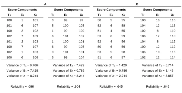
A simple example illustrates some possibilities. Table 1 compares hypothetical tests, each having a large number of scores with distributions like those shown in the table. In section A, the test on the left apparently has high true scores and low error scores, so that its reliability might be expected to be high, but, because the variance of T1 is much higher than that of E1, reliability is only .096.
the true scores at first glance look small. Nevertheless, despite the difference in reliability, the two tests have the same statistical power, because the observed-score variances are the same. In section B, the two tests have the same reliability, .645, because the variances of T and E, although different, have the same ratio. However, the observed-score variances are different, and the statistical power of the test on the left is greater.
Table 1. A) Score components of two tests having substantially different reliability coefficients and the same statistical power; B) Score components of two tests having the same reliability coefficients and substantially different statistical power.
A B
Score Components Score Components Score Components Score Components T1 E1 X1 T2 E2 X2 T1 E1 X1 T2 E2 X2 100 1 101 0 99 99 50 5 55 100 10 110 101 6 107 5 100 105 52 6 58 104 12 116 100 2 102 1 99 100 51 4 55 102 8 110 102 7 109 6 101 107 53 6 59 106 12 118 101 2 103 1 100 101 52 4 56 104 8 112 100 7 107 6 99 105 50 6 56 100 12 112 102 1 103 0 101 101 53 5 58 106 10 116 100 6 106 5 99 104 51 6 57 102 12 114
Variance of T1 − 0.786 Variance of T2 − 7.429 Variance of T1 − 1.429 Variance of T2 − 5.714
Variance of E1 − 7.429 Variance of E2 − 0.786 Variance of E1 − 0.786 Variance of E2 − 3.143
Variance of X1 − 8.214 Variance of X2 − 8.214 Variance of X1 − 2.214 Variance of X2 − 8.857
Reliability − .096 Reliability − .904 Reliability − .645 Reliability − .645
Power as a composite function of reliability
For investigating the relation of reliability and power, it is more convenient to examine changes in reliability with changes in true-score variance and error-score variance, as opposed to changes in observed-score variance as given by equations (1) and (2). It is then possible to express observed-score variance as a 1-1 function of reliability, provided either true-score variance or error-score variance is held constant. Then, because power is a 1-1 function of observed-score variance, it is possible in turn to express power as a composite function. Under those conditions, power is a monotonic decreasing function of observed-score variance and a monotonic increasing or decreasing function of reliability depending on which
component is constant. Of course, the form of the functions depends on properties of the particular hypothesis test considered.
First, begin with the equations
1 1 2 2 2 1 1 E / T E
and
2 2 2 2 2 2 1 E / T E
, solve both for 2 T , assumed to be constant, and set the two expressions equal. The result is
1 2 2 2 1 2 1 2 1 1 E E
Then, solving for ρ2 gives the result
2 1 2 2 2 1 1 1 1 E 1 E (5)
This equation indicates how reliability changes as the variance of the error component changes, while the true-score variance remains fixed.
Alternatively, if T2 changes while E2 is constant, a similar derivation give
1 1 2 2 2 1 T / T E
and
2 2 2 2 2 2 T / T E
, so that
1 2 2 2 1 1 2 2 1 / 1 / T T
. Solving for ρ2 gives the result1 2 2 2 2 1 1 1 1 T 1 T (6)
This equation indicates how reliability changes as true-score variance changes, while error-score variance is constant. Equations (5) and (6) clearly indicate that changes in reliability resulting from changes in either true-score variance or error-score variance depend only on the ratios
2 1
2 2
/
E E
or
T21/ T22 relating the old and new score components and not on the individual variances considered separately.Changes in observed score variability and power with
changes in reliability
Table 2 contains results found from equations (5) and (6). The first row at the top, labeled “Initial ρ” is the value of the reliability coefficient, denoted by ρ1 in the
equations, and the entries in the right-hand section of the table are the values of the new reliability coefficient, ρ2, after a designated change in the error-score
variance or true-score variance. The ratio of old-to-new error-score variance,
1 2
2 2
/
E E
, is located in the first column, and the entry in the table gives the value of the new reliability after the change, assuming that true-score variance remains constant. The same entry in the table is also the value of the new reliability if a change shown by the adjacent entry in the second column is made in the ratio1 2
2 2
/
T T
, assuming that error-score variance remains constant. That is, the ratios in the second columns are inverses of those in the first column, and the same change in reliability corresponds to both ratios.Table 2. Modification of reliability and observed-score variance by changes in error-score
variance (
E
E1 2
2 2
/ ) and in true-score variance (
T T1 2
2 2
/ ).Entries in the five right-hand
columns are the modified reliability values (ρ2) corresponding to variances and variance
ratios in the first four columns.
Initial Reliability (ρ1)
E
E 1 2 2 / 2 σ2 1 2 2 2 / T T
σ2 .10 .30 .50 .70 .90 0.250 5.000 4.000 1.250 .027 .097 .200 .368 .692 0.286 4.500 3.500 1.286 .031 .109 .222 .400 .720 0.333 4.000 3.000 1.333 .036 .125 .250 .438 .750 0.400 3.500 2.500 1.400 .043 .146 .286 .483 .783 0.500 3.000 2.000 1.500 .053 .176 .333 .538 .818 0.667 2.500 1.500 1.667 .069 .222 .400 .609 .857 1.000 2.000 1.000 2.000 .100 .300 .500 .700 .900 1.500 1.667 0.667 2.500 .143 .391 .600 .778 .931 2.000 1.500 0.500 3.000 .182 .462 .667 .824 .947 2.500 1.400 0.400 3.500 .217 .517 .714 .854 .957 3.000 1.333 0.333 4.000 .250 .562 .750 .875 .964 3.500 1.286 0.286 4.500 .280 .600 .778 .891 .969 4.000 1.250 0.250 5.000 .308 .632 .800 .903 .973values of σ2 decrease (and therefore power increases), as those of ρ
1 increase, and
vice versa. Also, the same values of ρ2 are associated with different values of σ2
(and therefore power).
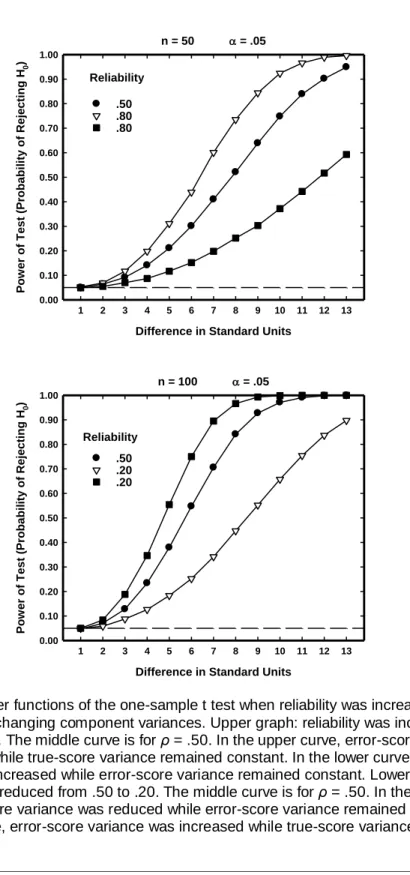
The relationship can be seen in more detail by plotting graphs of some power functions obtained from simulations. Figure 1 plots power functions of the one-sample Student t test under conditions where reliability was either increased or reduced by changing one component of the observed-score variance while the other remained constant. These simulations were programmed using Mathematica, version 4.1 (Wolfram, 1999), together with Mathematica statistical add-on packages. The program performed t tests on sums of “true-score” and “error-score” random variables, selected from N(0,1) and multiplied by constants in order to determine means, variances, and reliabilities. The means increased in increments of .32σ, and each data point in the figure was found from 20,000 iterations of the sampling procedure.
In both sections of the figure, the true-score and error-score variances were initially equal, so that reliability was .50. The middle curves with filled circles represent these initial reliabilities. In the upper section, reliability was increased to .80 in two ways. In the top curve in that section (triangular symbols), error -score variance was reduced, while true--score variance was constant. In the lower section (square symbols), true-score variance was increased while error-score variance was constant.
In the lower graph, reliability was decreased to .20 in two ways. In the top curve (square symbols), true-score variance was reduced while error-score variance was constant. In the lower curve (triangular symbols), error-score variance was increased while true-score variance was constant. All these curves, with shapes typical of power curves, show that the sum of the two variance components, that is, the observed-score variance, determined the power of the hypothesis test irrespective of how reliability changed as a result of a change in the ratio of the two components.
n = 50 = .05
Difference in Standard Units
1 2 3 4 5 6 7 8 9 10 11 12 13 Pow er of Tes t (Proba bil ity of Re ject ing H0 ) 0.00 0.10 0.20 0.30 0.40 0.50 0.60 0.70 0.80 0.90 1.00 .50 .80 .80 Reliability n = 100 = .05
Difference in Standard Units
1 2 3 4 5 6 7 8 9 10 11 12 13 Pow er of Tes t (Proba bil ity of Re ject ing H0 ) 0.00 0.10 0.20 0.30 0.40 0.50 0.60 0.70 0.80 0.90 1.00 .50 .20 .20 Reliability
Figure 1. Power functions of the one-sample t test when reliability was increased or decreased by changing component variances. Upper graph: reliability was increased
from .50 to .80. The middle curve is for ρ = .50. In the upper curve, error-score variance
was reduced while true-score variance remained constant. In the lower curve, true-score variance was increased while error-score variance remained constant. Lower graph:
Reliability was reduced from .50 to .20. The middle curve is for ρ = .50. In the upper
curve, true-score variance was reduced while error-score variance remained constant. In the lower curve, error-score variance was increased while true-score variance remained constant.
Relations, functions, and composite functions
It is well known that statistical power is a function of several variables, some of which are under the direct control of an experimenter. These include sample size,
N, the significance level, α, and the directionality of the hypothesis tested. Of course, different hypothesis tests, parametric and nonparametric, have different power characteristics under various conditions. The relations between N and power and between α and power are functional when the other variables are held constant; that is, each value in the domain of the relation is associated with a single value in its range. Some authors have considered it reasonable to add reliability to the list of determinants. However, as we have seen, reliability influences power only to the extent that it influences observed-score variance.
The association between reliability and power, therefore, is a mathematical relation, but it is not a function or a functional relation. However, it becomes functional if the variance of one of the two variables determining reliability is held constant. In that case, if the variance of one score component is held constant, power is a composite of two functions, the one between a score component and observed-score variance, and the one between observed-score variance and power. The range of the first function is the domain of the second.
As said before, still another way to express the same relationship is that, all other things equal, statistical power is a function of the sum of the variances of T
and E, whereas reliability is a function of the ratio of those two variances. As noted earlier, reliability can be defined as ψ/(ψ+ψ−1), where ψ = σT/σE. That definition makes it clear that reliability can be either large or small at the same time the sum, which determines power, is either large or small, independently of the ratio. The fact that power is determined by the observed-score variance, which is comprised of the sum in the denominator of the expression
T2 /
T2
E2
shows that, for a fixed value of E2, power has its maximum value when ρ = 0. But for a fixed value of T2 power has a maximum when ρ = 1.
Reliability of difference scores and statistical power
In order to gain insight into paradoxes concerning difference scores, we shall pursue an approach similar to the above. Rather than directly seeking a relationship between the reliability of differences and the power of an hypothesis test employing differences, we first consider how both are related to
observed-score variance and also the reliability coefficients of the two variables determining the differences.
Once again, beginning with what is known, the power of tests on difference scores, X − Y, is certainly a decreasing function of the variance of the difference scores. However, reliability depends on partitioning that variance into true and error components and finding ratios, which in turn depend on the similar ratios of both X and Y. In all cases, both reliability and the power of an hypothesis test can be considered joint functions of the true-score variance and error-score variance of the difference scores. However, power is determined uniquely by their sum and reliability by their ratio, just as in the case of a single variable X.
A familiar equation is 2 2 2 2 2 2 2 2 D X Y X Y X Y T T T T T T T D D X Y XY X Y
(7)where D = X − Y, TX and TY are the true score components of X and Y, and ρD is the reliability of D. If 2 2 X Y T T
and 2 2 X Y E E
, this equation can be solved for2 D
and substitutions made using 2 /
2 2
X X X X T T E
. The result is
2 2 2 1 X X Y T D T T X X
(8)and an equivalent result is
2 2 2 2 1 X Y D T T T E
(9)Although the assumption that variances of X and Y are equal is often unrealistic in practice, it suffices to indicate the form of the relation between reliability and statistical power. Next, the reliability of differences can be written in the form
1
, or 1 X Y X Y X T T D T T X (10)
2 2 2 1 1 X Y X Y T T T D T T T E (11)Equation (10) indicates that, if 0
X Y
T T
, the reliability of differences is the same as the common reliability of the components.
Equations (8), (9), (10), and (11) have the desirable feature that all combinations of values of the variables on the right-hand side of the equation yield meaningful values of ρD and 2
D
. That is not true in the case of several well-known formulas that involve both ρXY and ρX, because the Cauchy-Schwarz inequality places limits on the values the two can have together (Zumbo, 1999). For example, the relation
D
X
XY
/ 1
XY
is not meaningful for all values of ρXY and ρX.The above equations provide a convenient way to exhibit the relation between the reliability of differences and statistical power. Table 3 shows results of calculations using equations (9) and (11), comparing the reliability of component scores (ρX), the reliability of difference scores (ρD), and the observed variance of difference scores (D2 ), as a function of T2 while E2 is constant (upper section) and of E2 while T2 is constant (lower section).
If E2 is fixed, an increase in ρX comes from an increase in T2, and if T2 is fixed, it comes from a reduction in E2. Those outcomes are apparent in the table: As T2 increased from 0 to 1.8, the reliability coefficients ρX and ρD both increased, and also the variance of observed scores increased, so that statistical power decreased. The same was true for all three values of the correlation between true scores, ρ(TX,TY). On the other hand, as E2 increased from 0 to 1.8,
ρX and ρD both decreased, but the variance of observed scores still increased, so that power again decreased. As T2 varied, power was greatest when the reliability of differences was 0. However, as 2
E
varied, power was greatest when the reliability of differences was 1.
Table 3. Changes in observed variance and reliability of difference scores associated with changes in reliability of component scores.
ρ(TX,TY) = −.60 ρ(TX,TY) = 0 ρ(TX,TY) = .60 T 2 ρ X ρD D 2 ρ X ρD D 2 ρ X ρD D 2 0.0 .000 .000 2.000 .000 .000 2.000 .000 .000 2.000 0.2 .167 .242 2.640 .167 .167 2.400 .167 .074 2.160 0.4 .286 .390 3.280 .286 .286 2.800 .286 .138 2.320 0.6 .375 .490 3.920 .375 .375 3.200 .375 .194 2.480 1 E2 0.8 .444 .561 4.560 .444 .444 3.600 .444 .242 2.640 1.0 .500 .615 5.200 .500 .500 4.000 .500 .286 2.800 1.2 .545 .658 5.840 .545 .545 4.400 .545 .324 2.960 1.4 .583 .691 6.480 .583 .583 4.800 .583 .359 3.120 1.6 .615 .719 7.120 .615 .615 5.200 .615 .390 3.280 1.8 .643 .742 7.760 .643 .643 5.600 .643 .419 3.440 ρ(TX,TY) = −.60 ρ(TX,TY) = 0 ρ(TX,TY) = .60 E 2 ρ X ρD D 2 ρ X ρD D 2 ρ X ρD D 2 0.0 1.000 1.000 3.200 1.000 1.000 2.000 1.000 1.000 0.800 0.2 .833 .889 3.600 .833 .833 2.400 .833 .667 1.200 0.4 .714 .800 4.000 .714 .714 2.800 .714 .500 1.600 0.6 .625 .727 4.400 .625 .625 3.200 .625 .400 2.000 1 T 2 0.8 .556 .667 4.800 .556 .556 3.600 .556 .333 2.400 1.0 .500 .615 5.200 .500 .500 4.000 .500 .286 2.800 1.2 .455 .571 5.600 .455 .455 4.400 .455 .250 3.200 1.4 .417 .533 6.000 .417 .417 4.800 .417 .222 3.600 1.6 .385 .500 6.400 .385 .385 5.200 .385 .200 4.000 1.8 .357 .471 6.800 .357 .357 5.600 .357 .182 4.400
Consider now the relation between increases in reliability and power, reading from top to bottom in the columns in the upper section of the table and from bottom to top in the lower section. When the reliability coefficients of the component tests increased, the reliability of differences also increased, as long as just one column is considered. However, note that the same reliability of the components in many cases is associated with decidedly unlike reliabilities of the differences, depending on whether the change is attributable to a change in true-score variance or error-true-score variance. Often the values were far apart. Furthermore, the reliability of differences is either greater or less than that of the components, depending on whether the correlation between true scores, ρ(TX,TY), is positive or negative. As the absolute value of that correlation increases, the
The observed scores of the differences, and hence the statistical power,
increases as reliability increases if the change is attributable to a change in error-score variance and decreases if it is attributable to a change in true-score variance. That means that simply selecting a value of reliability, either of differences or the component tests, does not in itself provide information about the statistical power of the differences as a dependent variable. Just as in the case of a single test, the relation between reliability and power is not a functional relation unless the variance of one of the components of the scores is held constant.
These conclusions about the relation between power and the reliability of differences are consistent with results obtained by May & Hittner (2003), Overall & Woodward (1975, 1976), and Nicewander & Price (1978, 1983) using different methods. The so-called paradox of low reliability being associated with high power becomes more understandable from inspection of Table 3. That problem also is closely related to another issue that has been extensively treated in the literature, that of the reliability of differences often being considerably less than the reliability of the components. As the table shows, that is not always true, and again, looking at the reliability of the components alone, without further information, is one source of the trouble. The approach in Table 3, in which reliability coefficients are first related to the variances of true scores and error scores, makes it possible to focus on values that realistically would be likely to occur. At any rate, it is clear that an hypothesis test of differences can be powerful even if the reliability of a dependent variable is quite low.
How to increase statistical power: some practical
implications
As mentioned before, a possible reason for the controversies surrounding the relation of reliability and statistical power is ambiguity about the precise meaning of the term “reliability” in practical research. The term often is used in a way that conforms to popular usage, and even to widespread usage in various scientific fields, but does not match the mathematical definition given in classical test theory. The root of the difficulty is the fact that reliability, as defined in test theory, is a property of populations of individuals, that is a ratio of statistics applicable to populations, but not to a single individual or experimental object. The “reliability” of a scientific instrument, especially in physical sciences, often refers to its consistency in measuring a single physical object of a certain kind, but that is not the way the term is used in classical test theory.
When one asks the question “How does reliability influence power?” investigators in psychology and education often assume the question is similar to “How does reliability influence validity?” or “How does test length influence reliability?” What is typically desired is a function relating changes in the first variable to changes in the second variable, and many such functions are known in test theory. On the other hand, a researcher in another field, or a statistician, may assume the question is similar to “How does sample size influence power?” or “How does the significance level influence power?” having in mind well-known functions relating those variables.
As emphasized in the present note, there is not a unique way of making the increments in reliability needed to exhibit power as a function of reliability. We can conclude that increasing an instrument’s reliability will contribute to greater power in hypothesis testing only if the change occurs through a reduction of error-score variance that exceeds any increase in true-error-score variance occurring at the same time.
Suppose a researcher has a choice between two instruments, one with a known reliability coefficient of .90 and the other .80. Before assuming automatically that the first instrument is the better choice, it is prudent to look at the variance of scores that can be expected. If the instrument with lower reliability typically produces scores with considerably less variability, it could still be the better choice. That is especially true if the experiment is designed to detect possible differences among large groups of subjects with respect to an independent variable and is not concerned with short-term fluctuations in measures of individuals.
Another way to look at the problem is to recall that an hypothesis test is essentially a determination, based on probability, of whether or not a difference found between samples can be attributed to chance variability. However, an hypothesis test is blind to the partitioning of variability into contributions from separate components, such as “true scores” and “error scores.” A test statistic such as t typically is computed as a ratio of an obtained value to an estimate of variability based on a sampling distribution.
Recommending that the reliability coefficient be increased whenever possible is not always good advice in hypothesis testing, although the conventional emphasis on practical measures to reduce error variance still applies. All other things being equal, the more error of measurement can be avoided in an experiment, the better, and that task certainly should be considered along with other well-known methods of increasing power (see, for example, Wilcox, 2003)
the same practical steps also reduce observed-score variance. If a more heterogeneous group is tested at the same time error of measurement is less, power does not necessarily increase. For practical usefulness, eliminating error and thereby increasing reliability for a particular population of examinees can be effective, provided the change is made without altering the population.
References
Cleary, T. A., & Linn, R. L. (1969). Error of measurement and the power of a statistical test. British Journal of Mathematical and Statistical Psychology,
22(1), 49-55. doi:10.1111/j.2044-8317.1969.tb00419.x
Cohen, J. (1988). Statistical power analysis for the behavioral sciences (3rd ed.). Englewood Cliffs, NJ: Lawrence Erlbaum Associates.
Collins, L. M. (1996). Is reliability obsolete? A commentary on “Are simple gain scores obsolete?” Applied Psychological Measurement, 20(3), 289-292. doi:10.1177/014662169602000308
Feldt, L. S. & Brennan, R. L. (1989). Reliability. In R. L. Linn (Ed.),
Educational measurement (3rd ed., pp. 105-146). New York: Macmillan. Fleiss, J. J. (1976). Comment on Overall & Woodward’s asserted paradox concerning the measurement of change. Psychological Bulletin, 83(5), 774-775. doi:10.1037/0033-2909.83.5.774
Gulliksen, H. (1950). Theory of mental tests. New York: Wiley.
Hopkins, K. D., & Hopkins, D. R. (1979). The effect of the reliability of the dependent variable on power. Journal of Special Education, 13(4), 463-466. doi:10.1177/002246697901300413
Kopriva, R. J., & Shaw, D. G. (1991). Power estimates: The effect of dependent variable reliability on the power of one-factor ANOVAs. Educational and Psychological Measurement, 51(3), 585-595.
doi:10.1177/0013164491513006
Levin, J. R. (1986). Note on the relation between the power of a significance test and the reliability of the measuring instrument. Multivariate Behavioral Research, 21(2), 255-261. doi:10.1207/s15327906mbr2102_6
Lord, F. M., & Novick, M. R. (1968). Statistical theories of mental test scores. Reading, MA: Addison-Wesley.
May, K., & Hittner, J. B. (2003). On the relation between power and reliability of difference scores. Perceptual and Motor Skills, 97(3.1), 905-908. doi:10.2466/PMS.97.7.905-908
Mellenbergh, G. J. (1996). Measurement precision in test score and item response models. Psychological Methods, 1(3), 293-299.
doi:10.1037/1082-989X.1.3.293
Mellenbergh, G. J. (1999). A note on simple gain score precision. Applied Psychological Measurement, 23(1), 87-89. doi:10.1177/01466216990231007
Nicewander, W. A., & Price, J. M. (1978). Dependent variable reliability and the power of statistical tests. Psychological Bulletin, 85(2), 405-409. doi:10.1037/0033-2909.85.2.405
Nicewander, W. A., & Price, J. M. (1983). Reliability of measurement and the power of statistical tests. Psychological Bulletin, 94(3), 524-513.
doi:10.1037/0033-2909.94.3.524
Novick, M. R. (1966). The axioms and principal results of classical test theory. Journal of Mathematical Psychology, 3(3), 1-18.
doi:10.1016/0022-2496(66)90002-2
Overall, J. E., & Woodward, J. A. (1975). Unreliability of difference scores: A paradox for measurement of change. Psychological Bulletin, 82(1), 85-86. doi:10.1037/h0076158
Overall, J. E., & Woodward, J. A. (1976). Reassertion of the paradoxical power of tests of significance based on unreliable difference scores.
Psychological Bulletin, 83(5), 776-777. doi:10.1037/0033-2909.83.5.776
Subkoviak, M. J., & Levin, J. R. (1977). Fallibility of measurement and the power of a significance test. Journal of Educational Measurement, 14(1), 47-52. doi:10.1111/j.1745-3984.1977.tb00028.x
Sutcliffe, J. P. (1958). Error of measurement and the sensitivity of a test of significance. Psychometrika, 23(1), 9-17. doi:10.1007/BF02288974
Thomas, D. R., & Zumbo, B. D. (2012). Difference scores from the point of view of reliability and repeated measures ANOVA: In defense of difference scores for data analysis. Educational and Psychological Measurement, 72(1), 37-43. doi: 10.1177/0013164411409929
Wilcox, R. B. (2003). Applying contemporary statistical techniques. New York: Academic Press.
Zimmerman, D. W., & Williams, R. H. (1986). Note on the reliability of experimental measures and the power of significance tests. Psychological Bulletin, 100(1), 123-124. doi:10.1037/0033-2909.100.1.123
Zimmerman, D. W., Williams, R. H., & Zumbo, B. D. (1993). Reliability of measurement and power of significance tests based on differences. Applied Psychological Measurement, 17(1), 1-10. doi:10.1177/014662169301700101
Zumbo, B. D. (1999). The simple difference score as an inherently poor measure of change: Some reality, much mythology. In B. Thompson (Ed.).
Advances in Social Science Methodology, 5, (pp. 269-304). Greenwich, CT: JAI Press.
Dr. Knapp is Professor Emeritus of Education and Nursing at the University of Rochester
Invited Article
In (Partial) Defense of .05
Thomas R. Knapp University of Rochester Rochester, NYResearchers are frequently chided for choosing the .05 alpha level as the determiner of statistical significance (or non-significance). A partial justification is provided.
Keywords: .05 level, statistical significance, R. A. Fisher
Introduction
For the last 50 or 60 years it has been fashionable to deride the insistence on using an alpha level of .05 for testing the statistical significance of a sample finding. It is commonplace to read critical comments such as “The current obsession with .05” (Skipper, Guenther, & Nass, 1967, p. 16; see also Labovitz, 1968) and “God loves the .06 nearly as much as the .05” (Rosnow & Rosenthal, 1989, p. 1277). In the spirit of Robinson, Funk, Halbur, and O'Ryan (2003) I would like to provide an explanation for ‘why .05?’ and an argument in favor of its prevailing use. Near the end of the paper I will give a similar argument for 95% confidence (.05's interval estimation counterpart), and I will conclude with a few cautionary statements regarding total devotion to .05 and/or 95%.
A bit of history
Although there is some evidence for earlier recommendations of .05 as a defensible level of statistical significance, most people claim that it was first suggested by Fisher (1926):
[T]he evidence would have reached a point which may be called the verge of significance; for it is convenient to draw the line at about the
level at which we can say 'Either there is something in the treatment or a coincidence has occurred such as does not occur more than once in twenty trials.' This level, which we may call the 5 per cent level point, would be indicated, though very roughly, by the greatest chance deviation observed in twenty successive trials... If one in twenty does not seem high enough odds, we may, if we prefer it, draw the line at one in fifty (the 2 per cent point) or one in a hundred (the 1 per cent point). Personally, the writer prefers to set the low standard of significance at the 5 per cent point, and ignore entirely all results which fail to reach this level. (p. 504)
There are several things to note about what Fisher said:
1. He used the interesting phrase “the verge of significance”. As far as I have been able to determine, none of his critics have commented about that choice of words.
2. He did not insist on .05, as the second part of the quote indicated. Many of his critics unfairly charged him with being unwavering regarding .05.
3. Surprisingly, he confused probability with odds (and high with low). The alpha level of .05 has to do with a probability of one in twenty; the corresponding odds are one to nineteen (in favor) or nineteen to one (against).
Fisher didn’t write about .05 being the probability of making a Type I error. That concept (along with the probability of making a Type II error) was yet to come in the Neyman-Pearson approach to hypothesis testing. Also yet to come were several acrimonious arguments between Fisher and W. S. Gosset (who had previously developed the t-test), between Fisher and Karl Pearson, and between Fisher and both Jerzy Neyman and Egon Sharpe Pearson (Karl’s son), as documented by Fienberg and Tanur (1966), Cowles and Davis (1982), Inman (1994), Wainer and Robinson (2003), and others.
In the intervening years between 1926 and the present there were several criticisms of .05, e.g., Cohen (1994), along with some defenders, e.g., Robinson, et al. (2003). Cohen (1994) was particularly puzzling (see the collection of comments regarding it in the December, 1995 issue of American Psychologist). The title is difficult to understand. Was he trying to be clever in considering “The earth is round” as a null hypothesis that should be rejected at the .05 level,
because it is actually slightly elliptical rather than perfectly round? He also made an error where he claimed many people believe a p-value is the probability that the null hypothesis is false. No; some people mistakenly believe that a p-value is the probability that the null hypothesis is true; no one believes p is the probability of a false null.
After discussing some of the historical origins of the use of an alpha level of .05, Robinson, et al. (2003) provided the results of empirical studies in which students were asked how many heads in each of the first n flips of a coin would lead them to claim that the coin was not “fair”. The modal response in most of those studies was five. The probability of heads on the first five tosses of a fair coin is .03125, which is close to the traditional .05 (see Figure 1 below).
A rationale for .05
Although Fisher didn't use the following argument, some of the students in the Robinson, et al. (2003) studies apparently did, implicitly if not explicitly. (Comparable arguments have been made by Tintle, et al., 2014 and at the EMBstats website, http://www.embstats.com. See Figure 1 below for the latter.) Suppose you were asked your opinion about the fairness of a coin. You want to make a decision if its probability of landing as heads is equal to .5. How many heads would have to be obtained in the first five tosses for you to call a halt and conclude it’s not a fair coin? The probability of one head in one toss of a fair coin is .5. (You wouldn’t call a halt.) The probability of two heads in two tosses is .5 × .5 = .25, and the probability of three heads in three tosses is .5 × .5 × .5 = .125. (Still no clear decision to halt.) The probability of four heads in four tosses is .5 × .5 × .5 × .5 = .0625. (Perhaps the decision to halt is near, and note .0625 is close to .05.) If you want to wait for the result of one more toss, the probability of five heads in five tosses is .5 × .5 × .5 × .5 × .5 = .03125. At this point you are likely to claim that the coin is not fair. (The difference between .0625 and the .03125 is .046875, which is very close to .05.) However, you know you might be wrong.
Figure 1 details the argument presented at the EMBstats website. Note the interpretations of “Unusual” (for 4 heads in 4 tosses), “Surprising” (for 5 heads in 5 tosses), “Strange” (for 6 heads in 6 tosses), and “I don't believe it!” (for 7 heads in 7 tosses). Fisher’s .05 would come between “Unusual” and “Surprising”. He avoided the matter of proof and exhibited a commendable tolerance for uncertainty. Similarly, statisticians are so comfortable with uncertainty that they