A comparative analysis of TRMM-rain gauge data merging techniques at the daily time scale for distributed rainfall-runoff modelling applications

A Comparative Analysis of TRMM–Rain Gauge Data Merging Techniques at the Daily

Time Scale for Distributed Rainfall–Runoff Modeling Applications

DANIELENERINI,*,1,##ZEDZULKAFLI,*,#LI-PENWANG,*,@CHRISTIANONOF,* WOUTERBUYTAERT,*,& WALDOLAVADO-CASIMIRO,**ANDJEAN-LOUPGUYOT11

* Department of Civil and Environmental Engineering, Imperial College London, London, United Kingdom

1_{Federal Office of Meteorology and Climatology MeteoSwiss, Locarno-Monti, Switzerland}

#_{Department of Civil Engineering, Universiti Putra Malaysia, Serdang, Malaysia} @_{Hydraulics Laboratory, Katholieke Universiteit Leuven, Leuven, Belgium}

&_{The Grantham Institute on Climate Change and the Environment, Imperial College London, London, United Kingdom}

** Servicio Nacional de Meteorologı´a e Hidrologı´a, Lima, Peru

11_{Institut de recherche pour le développement, Lima, Peru}

(Manuscript received 10 October 2014, in final form 25 March 2015) ABSTRACT

This study compares two nonparametric rainfall data merging methods—the mean bias correction and double-kernel smoothing—with two geostatistical methods—kriging with external drift and Bayesian combination—for optimizing the hydrometeorological performance of a satellite-based precipitation product over a mesoscale tropical Andean watershed in Peru. The analysis is conducted using 11 years of daily time series from the Tropical Rainfall Measuring Mission (TRMM) Multisatellite Precipitation Analysis (TMPA) research product (also TRMM 3B42) and 173 rain gauges from the national weather station network. The results are assessed using 1) a cross-validation procedure and 2) a catchment water balance analysis and hy-drological modeling. It is found that the double-kernel smoothing method delivered the most consistent im-provement over the original satellite product in both the cross-validation and hydrological evaluation. The mean bias correction also improved hydrological performance scores, particularly at the subbasin scale where the rain gauge density is higher. Given the spatial heterogeneity of the climate, the size of the modeled catchment, and the sparsity of data, it is concluded that nonparametric merging methods can perform as well as or better than more complex geostatistical methods, whose assumptions may not hold under the studied conditions. Based on these results, a systematic approach to the selection of a satellite–rain gauge data merging technique is proposed that is based on data characteristics. Finally, the underperformance of an ordinary kriging interpolation of the rain gauge data, compared to TMPA and other merged products, supports the use of satellite-based products over gridded rain gauge products that utilize sparse data for hydrological modeling at large scales.

1. Introduction

Hydrological studies rely on the quality of rainfall estimates to produce meaningful modeling output. Rain gauges can deliver accurate point measurements, but

their poor ability to describe the spatial structure of rainfall can be a major limitation when precipitation fields are required, for example, in distributed hydro-logical modeling applications. This problem is more severe in tropical regions because of high rainfall vari-ability and scarce data conditions.

Satellite-based estimates such as the Tropical Rainfall Measuring Mission (TRMM) Multisatellite Precipitation Analysis (TMPA; also TRMM 3B42) product are becom-ing increasbecom-ingly attractive as an alternative source of forc-ing data in data-sparse regions, although their application

##_{Current affiliation: Cat Perils, Swiss Reinsurance Company,}

Ltd., Zurich, Switzerland.

Corresponding author address:Daniele Nerini, Cat Perils, Swiss Reinsurance Company, Ltd., Mythenquai 50/60, Zurich CH-8022, Switzerland.

E-mail: [email protected] Denotes Open Access content.

This article is licensed under aCreative Commons Attribution 4.0 license.

DOI: 10.1175/JHM-D-14-0197.1 Ó2015 American Meteorological Society

can be limited by quantitative inaccuracies (Zulkafli et al. 2014a;Anagnostou et al. 2010;Tian et al. 2007). Information from a large number of rain gauges is already assimilated as part of global/regional satellite algorithms; nevertheless, the rain gauge databases sourced by these procedures can ex-clude more extensive national networks where data acces-sibility is restrictive, as often is the case in developing countries. In these regions, the global precipitation product may be found to be unsatisfactory and requiring local ad-justment (e.g.,Lavado-Casimiro et al. 2009).

Satellite algorithms are known to internally perform gauge correction, for example, using a mean-field bias correction (MBC) and/or inverse-error-weighted aver-aging methods (Huffman et al. 1997;Grimes et al. 1999). Postanalysis merging methods have also been used on the products of these algorithms, for example, the spatial adjustment of TMPA using interpolations by inverse distance weighting (Lavado-Casimiro et al. 2009), double-kernel smoothing (DS; Li and Shao 2010), and the nearest neighbor method (Vila et al. 2009); correc-tion through regression analysis between the satellite-and rain gauge–based precipitation at various temporal scales, for example, climatologies in Almazroui (2011)

and monthly inYin et al. (2008); and correction using probability distributions (Anagnostou et al. 1999). Geo-statistical methods have also been used such as the kriging with external drift (KED) to combine gauge and 10-day (dekad) IR-based precipitation data from Me-teosat (Grimes et al. 1999) and the cokriging approach to interpolate daily rain gauge data with the GPCP multisatellite precipitation estimates as covariates (Kottek and Rubel 2008). More recently, Heidinger et al. (2012)performed a wavelet analysis on the signals from daily rain gauge and TMPA time series and reconstructed a combined product by overlaying short-term noise from the gauge signal on the long-short-term trends in the TMPA signal.

The methods applied to satellite data have origins in the radar research community, for example, MBC [ref-erences in Gjertsen et al. (2004)], spatial adjustment (Moore et al. 1989;Wood et al. 2000), KED (Haberlandt 2007;Erdin 2009;Schiemann et al. 2011;Goudenhoofdt and Delobbe 2009), and cokriging (Krajewski 1987). A particularly promising technique that has not been largely applied to satellite-based rainfall estimation is the Bayesian combination (BC) method proposed by

Todini (2001). This method quantifies the estimation uncertainties of precipitation data measured by differ-ent sensors (e.g., satellite, radar, and ground rain gauges), then combines these data such that the overall estimation uncertainty formulated in terms of estima-tion error covariances is minimized. Promising results from this method have been obtained from both

numerical examples (Mazzetti and Todini 2004) and case studies in a small-scale densely gauged urban catchment (Wang et al. 2013).

Despite the wealth of merging algorithms at our disposal, there is not a clear guideline as to which method would be optimal given the data characteristics (density, spatial bias, temporal resolution, etc.). In this study, we compare two nonparametric rainfall data merging methods—MBC and DS—with two geostatistical methods—KED and BC (un-tested for satellite applications)—over a mesoscale tropical Andean catchment in Peru. The analysis is conducted using 11 years of available data from the TMPA, version 7, research product and 173 rain gauges in the national weather station network of Peru. The results are assessed through a cross-validation procedure and supplemented by a hydrological evaluation using the catchment water balance and a hydrological model. The aim is to highlight the strengths and weaknesses of each of the methods and provide some guidelines for a pre-liminary selection of methods in the context of data-sparse hydrological applications.

2. Data and methods

a. Study area

This study focuses on a mesoscale river basin that spans the Peruvian Andes and the Amazon floodplains (Fig. 1). The Peruvian Amazon (locally Marañón) River basin extends from latitude 18to 118S and from longi-tude 808to 748W, covering about 360 000 km2_{. The} alti-tude of the basin ranges from well above 4000 m MSL in the western boundary in the Andes to the Amazonian floodplains to the east.

The downstream limit of the hydrological basin is defined by the gauging station at San Regis (4.48S, 748W). Upstream, the river is gauged at three other stations: Borja, Santiago, and Chazuta. Farther down-stream, the Marañón River merges with the Ucayali River to form the Amazon River just before reaching the city of Iquitos. The basin covers the Pacaya–Samiria National Reserve, which is the largest floodable forest reserve in Peru and is an area of high ecological significance.

A complex climatic pattern is present in the region because of the interaction between various synoptic meteorological processes and the orographic effect of the Andes. In general, rainfall is particularly high in regions close to the equator (more than 2000 mm yr21) because of the passage of the intertropical conver-gence zone (ITCZ) and decreases toward the tropics (Espinoza Villar et al. 2009). Additionally, humid At-lantic trade winds flow east–west across the vast rain forest and form an intense orographic belt along the

eastern Andes as they encounter the first slopes (Espinoza Villar et al. 2009; Garreaud et al. 2009;

Bookhagen and Strecker 2008). They also deviate south-ward, transporting moist air toward the subtropics. In the highlands, the Andean landscape causes shielding and moisture intensification resulting in various microclimates (Buytaert et al. 2006a;Rollenbeck and Bendix 2011). b. Precipitation data

The satellite-based product is obtained from the TMPA product, in its latest available version 7, released in November 2012. The TMPA product combines ob-servations from multiple satellites, including TRMM and other geostationary satellites (Huffman and Bolvin 2013). The performance of this dataset in this study area has been previously assessed byZulkafli et al. (2014a). Precipitation estimates from 1998 to 2008 were obtained with a 3-h temporal resolution and 0.258 3 0.258 (ap-proximately 27.8 km 3 27.8 km) spatial resolution. Values were subsequently aggregated to the daily scale in order to match the temporal resolution of the rain gauge records.

The rain gauge dataset is the historical rainfall time series obtained from the Peruvian National Meteorological

and Hydrological Service [Servicio Nacional de Meteorología e Hidrología del Perú(SENAMHI)]. This includes daily rainfall amounts in millimeters for 11 years between January 1998 and December 2008 from 173 recording stations located within the satellite do-main. Their locations are shown in Fig. 1. The area covered by the rain gauges is about 1 100 000 km2, which translates to an average network density of less than one rain gauge per 5000 km2. The gauges are particularly clustered around towns and along rivers, providing higher densities in regions of easier access. The high-lands are also better represented compared to the low-lands, as the average rain gauge altitude of 1560 m MSL indicates (Table 1).

c. Merging methods

The methods compared are 1) MBC, 2) DS, 3) ordi-nary kriging (OK; rain gauge interpolation only), 4) KED, and 5) BC.

1) MEAN BIAS CORRECTION

This method corrects the satellite-based product by the total multiplicative bias between the rain gauge estimates and the collocated satellite values, thus FIG. 1. The Marañón basin and three subbasins. The map includes the regional topography, the

assuming a uniform bias over the spatial domain. For each daily event (i.e., each time step), a correction factor Bis thus calculated using the following equation:

B5

å

N j51 Z_G(x_j)

å

N j51 Z_S(x_j) , (1)

where Nis the number of available gauges inside the satellite domain, andZG(xj) andZS(xj) are the gauge and satellite daily rainfall values corresponding to gauged locationj.

2) DOUBLE-KERNEL SMOOTHING

The nonparametric double-kernel smoothing is a tech-nique developed by Li and Shao (2010) specifically for data-sparse applications. The main idea of this method is the interpolation of the point residuals«Susing the kernel density function and the adjustment of the satellite field by the estimated residual field. The point residual at the given gauged locationj51,. . .,Nis defined to be

«_S

j5

«_S(x_j)5Z_S(x_j)2Z_G(x_j) . (2) A first-level interpolation is performed to generate a full set of residuals (pseudoresiduals) «SS on the same grid as the satellite data. At the given gridpoint location i51,. . .,M, the pseudoresidual is defined to be:

«_SS i5

å

N j51 L(kH_i2H_jk/b)«_S j

å

N j51 L(kH_i2H_jk/b) , (3)

where kkis the Euclidean norm andL is the Kernel function defined as a Gaussian kernel followingLi and Shao (2010): L(kH_i2H_jk/b)5 1ffiffiffiffiffiffi 2p p exp 21 2(kHi2Hjk/b) 2 . (4)

The variable His the position of the points, and the bandwidth b is determined using Silverman’s rule of thumb (Silverman 1998): b5 4s5 3n 1/5 , (5)

wherenis the number of samples andsis the standard deviation of samples. A second-level interpolation is applied on both the residuals and pseudoresiduals to estimate the final error field«DS:

«_DS k5

å

N j51 L(kH_k2H_jk/b₁)«_S j1

å

M i51 L(kH_k2H_ik/b₂)«_SS i

å

N j51 L(kH_k2H_jk/b₁)1

å

M i51 L(kH_k2H_ik/b₂) , (6) and the merged productZDSat pointkis calculated by subtracting to the satellite estimate ZSk the

corre-sponding error«DSk:

Z_DS

k5ZSk2

«_DS

k. (7)

The kernel smoothing (interpolation) of the residuals does not rely on the stationary assumption, as is the case for geostatistical methods. The formulation is such that the product of the merging will converge toward the rain gauge estimates with decreased distance toward the ground observations.

3) ORDINARY KRIGING

Among kriging estimation methods, the ordinary kriging provides the best unbiased linear estimates of point values or block averages (where ‘‘best’’ means minimum variance). The basic assumption of the OK is that data values can be characterized using a stationary random variable with an unknown mean (Müller 2007). Here, the OK is used to produce the rainfall estimates at each satellite grid location through the interpolation of discrete (point or grid averaged) rain gauge measure-ments. These spatially interpolated rain gauge esti-mates, along with the original satellite product, then serve as the baseline for comparison with the merged products.

Ordinary kriging uses the (semi) variogram to char-acterize the spatial association of data values at different locations. The definition of the (isotropic) semivario-gram is given as follows:

TABLE1. Key characteristics of the rain gauge dataset. Values are indicative of the available period (1998–2008).

No. of stations Mean altitude (m MSL) Mean annual rainfall (mm) Max intensity (mm day21_{) Missing values (%)}

173 1560 1350 216.8* 8.3

g(h)51

2var[Z(x1h)2Z(x)] , (8) whereg is the semivariance of the random variableZ between two points with distanceh. Note thatgdoes not depend on the positionx, but it is only a function of distanceh, thus assuming stationarity of the variance of the differences separated by the same distance. In this case, we also assume the isotropy of the model, sincegis not function of the direction. The variogram can be empirically estimated from available observations by computing the semivariance g for several classes of distances between gauges. This is known as experi-mental or empirical variogram.

Once the experimental variogram is estimated, it is possible to fit a theoretical variogram model to it. In the literature there are a variety of different models: see de Marsily (1986) for a complete list. In this study, the exponential model was found to produce the best fit:

g(h)5v[12exp(2h/a)] , (9)

whereadenotes the range, the distance after which the variogram reaches its asymptotic value, the sillv, so that the correlation between farther apart gauges is approximately equal to zero. A nugget effect can be added to Eq.(9) to represent any residual vari-ance not explained by distvari-ance at an infinitesimally small separation, due to measurement and epistemic errors.

The unknown precipitation valueZ* at locationx0is estimated as a linear combination of the precipitation valuesZG(xj) at known pointsxj, weighted by the sem-ivariogram functionl(h):

Z*(x₀)5

å

N j51

l_jZ_G(x_j) . (10)

The only additional constraint is that the weights have to add up to unity:

å

N

j51

l_j51 . (11)

This condition is necessary to guarantee an unbiased estimator (de Marsily 1986). Equation(10), subjected to Eq.(11), is solved by minimizing the variance of the estimation errors var(ZG* 2ZG), which are assumed to

have a Gaussian distribution. The resulting OK equa-tion is thus the following:

å

N

j51

l_jg(x_i,x_j)1m5g(x_i,x₀) , (12)

where m is the Lagrange multiplier used to fulfill the unbiased condition [Eq.(11)]. Equation(12)can be re-written in the matrix form A3x5b, so that the un-knownxrepresents the set of weights in Eq.(10),Ais the semivariogram matrix with a term for each pairs of gauges, andbis the semivariogram vector between all gauges and the prediction pointx0:

0 B B B B B B @ 0 g₁₂ g₁₃ ⋯ g_1N 1 g₂₁ 0 g₂₃ ⋯ g_2N 1 ... ... ... ⋱ ... ... g_N1 g_N2 g_N3 ⋯ 0 1 1 1 1 ⋯ 1 0 1 C C C C C C A 3 0 B B B B B B B @ l1 0 l2 0 ... lN 0 m 1 C C C C C C C A 5 0 B B B B B B @ g₁₀ g₂₀ ... g_N0 1 1 C C C C C C A , (13) where gij denotes g(xi,xj), the semivariogram value between two known pointsiandj.

The way the equation is set up is such that the solution may include negative weights, which can distort the final estimated values. Hence, an a posteriori correction to the weights is performed according to the algorithm proposed byDeutsch (1996).

4) KRIGING WITH EXTERNAL DRIFT

KED is an extension of the OK whereby non-stationarity is assumed and represented by the drift term, which in our case is the satellite-based estimates.

The method implemented is as described inHewitt (2012). KED requires the satellite value at the pre-diction locationx0to be equal to the weighted average of the satellite valuesZSat gauged locationsxj:

å

N

j51

l_jZ_S(x_j)5Z_S(x₀) . (14)

This additional condition is included in the error min-imization equation [Eq.(12)] to produce the following:

å

N

j51

l_jg(x_i,x_j)1m_a1m_bZ_S(x_i)5g(x_i,x₀) . (15)

0 B B B B B B B B @ 0 g₁₂ g₁₃ ⋯ g_1N 1 Z_S,1 g₂₁ 0 g₂₃ ⋯ g_2N 1 Z_S,2 ... ... ... ⋱ ... ... ... g_N1 g_N2 g_N3 ⋯ 0 1 Z_S,N 1 1 1 ⋯ 1 0 0 Z_S,1 Z_S,2 Z_S,3 ⋯ Z_S,N 0 0 1 C C C C C C C C A 3 0 B B B B B B B @ l1 0 l2 0 ... lN 0 m_a m_b 1 C C C C C C C A 5 0 B B B B B B B @ g₁₀ g₂₀ ... g_N0 1 Z_S,0 1 C C C C C C C A , (16)

whereZS,idenotesZS(xi), the satellite-based estimation at locationi. For the interpolation,ZS(xi) andZS(xj) are used solely for their covariance for weighting values of

ZG(xi); the actual values ofZS(xi) do not feed into the final estimates.

5) BAYESIAN COMBINATION

The theory underpinning the Bayesian combination method is described inTodini (2001)andPROGEA Srl (2009)and summarized here. This method first uses the block kriging method to generate interpolated rain gauge rainfall estimates at each satellite grid location and to estimate the associated estimation error co-variance (i.e., estimation uncertainty).

After kriging interpolation, the Kalman filter (Kalman 1960) is then employed to merge these esti-mates with the coincidental satellite rainfall product by comparing the uncertainty of these two data sources. Here the merged product becomes the a posteriori es-timatey00, which is defined as

y005Z_S1K(Z_G2Z_S2m_«) , (17) wherem«is the mean of the satellite–rain gauge bias [i.e., E(ZG 2ZS)] and Kis the Kalman gain. The Kalman gain represents the relative measure of uncertainty and is defined as follows:

K5V«_S(V«_S1V«_G)21. (18)

The uncertainty associated with the satellite estimates V«S is represented by the covariance matrix of the

sat-ellite error field (i.e., «5ZG2ZS), while the un-certainty associated with the rain gauge rainfall estimates V«G is the error variance produced in the

kriging interpolation. The variable K increases (de-creases) asV«_Sis larger (smaller) compared toV«_G, and consequently, the filter will weigh more in favor of the rain gauge (satellite) estimates in the combination.

The Bayesian combination method was initially implemented using the commercial software RAIN-MUSIC (PROGEA Srl 2009). As the software is not open source, the default settings of the method cannot be changed, for example, the theoretical variogram

model for the kriging interpolation has to be Gaussian. A MATLAB script was thus implemented to execute the Bayesian combination with several changes: 1) Instead of the Gaussian variogram model, the

expo-nential variogram model was found to provide a better fit to the experimental variogram for the kriging interpolation.

2) Instead of using the block kriging method, the OK method was used to interpolate grid-averaged rain gauge data. The main difference between the ordi-nary and block kriging methods lies in the way variograms are calculated from data. The former calculates the variance between two points, while the latter calculates the variance between point and block (which is the average of the point-to-point variances).

To distinguish the two different implementations, the RAINMUSIC Bayesian combination will be sub-scripted as BCR, whereas the replicate (MATLAB) model is annotated as BC.

d. Meteorological evaluation

Since we do not know the true rainfall value at a given grid point, we employed collocated rain gauge obser-vations as a first approximation in order to assess the accuracy of the various merged precipitation products. The reader should nonetheless be aware of the scale mismatch that exists between rain gauge point mea-surements and 0.258 satellite cells (approximately 773 km2in TMPA). However, in our context of a com-parative evaluation, the pixel-to-point evaluation is implemented in the same fashion across all four merging methods and therefore is not expected to affect the relative performance.

The collocation of a rain gauge to a satellite grid cell was performed using nearest neighbor approximation, such that rain gauges are associated to the centers of the nearest grid cells. If multiple gauges are present over the same cell, their estimates are averaged to produce a presumably more representative value.

The satellite–gauge data merging was tested in a 10-fold cross-validation scheme. The cross validation was performed at the daily time step for 141 days of rain,

during which more than 75% of the rain gauges recorded a rain event.

The goodness-of-fit between the merged products and the corresponding pixel-average rain gauge values was evaluated in terms of the mean absolute error MAE, mean error ME, root-mean-square error RMSE, Nash– Sutcliffe efficiency NSE, and percent bias (relative bias in percent).

An analysis of error components such as false alarms and missed events is not included. This would require a detailed discussion of each of the merging techniques on those performance indices, which is beyond the scope of this study. From a hydrological modeling perspective, this should not represent an issue given the large scale of the studied basins. Both false alarms and missed events are typically dominated by low-intensity or very local-ized events (covering part of the pixel but missed by the rain gauge or vice versa) which have only a limited contribution to streamflow. If they indeed have a hy-drological impact (e.g., on the water balance and flow magnitude), then this should be captured in the perfor-mance metrics included in the analysis. However, for smaller-scale applications, such error components might have an impact. The reader is referred toMaggioni et al. (2013)for a related analysis.

e. Hydrological evaluation

A first-level hydrological assessment of the data quality was conducted using the catchment water bal-ance with the runoff ratio RR defined as the ratio of the precipitation that contributes to runoff:

RR5R

P. (19)

The RR values calculated using the different outputs from the merging were compared to known values from the literature (Campling et al. 2002; Buytaert et al. 2006b;Rollenbeck and Anhuf 2007).

The merged precipitation products were subsequently used to drive a hydrological model. The Joint UK Land Environment Simulator (JULES; Best et al. 2011), which is a physics-based community model derived from the Met Office land surface scheme, was parameterized over 2040 grid boxes of 0.1258 30.1258(approximately 14 km3 14 km) in the catchment using best-available land cover and soil data to generate runoff. The runoff was then routed offline along the river network using a delay function to simulate streamflows at various points in the river basin. The river network was developed using hydrographic data (90-m resolution) from the Hydrological Data and Maps Based on Shuttle Eleva-tion Derivatives at Multiple Scales (HydroSHEDS;

Lehner et al. 2008). Model optimization was only used to obtain the routing parameters (flood wave celerities); any inconsistent model compensation of the pre-cipitation errors across the merging products is not ex-pected. For further description of the model, the reader is referred toZulkafli et al. (2013).

The impact of merged precipitation forcing data on streamflow simulations is assessed by comparison with observed daily discharges. The evaluation is done at four streamflow gauging stations, identified inFig. 1, over an 11-yr period (1998–2008). Streamflow data were obtained through Geodynamical, Hydrological, and Biogeochemi-cal Control of Erosion/Alteration and Material Transport in the Amazon Basin (HYBAM) from SENAMHI and the Instituto Nacional de Meteorología e Hidrología, Ecuador (INAMHI), monitoring networks. The goodness-of-fit was evaluated in terms of the percent bias (relative bias in percent), correlation, RMSE, and NSE at the daily scale.

f. Software

The merging algorithms in this study were originally written in MATLAB. Subsequently, these have been rewritten in R and made publicly available on GitHub (Zulkafli et al. 2014b).

3. Results

a. Spatial variability of precipitation

A spatial analysis of the mean annual precipitation across the merged products is presented inFig. 2. The figure shows MBC and DS retaining a high degree of information from TMPA, whereas KED and BCR re-semble more closely the OK field. These patterns from MBC, DS, and KED are reasonable, given that the MBC and DS methods consider the entire satellite rainfall field information in the adjustment process, while KED only uses the satellite information at gauging locations as an external drift term. However, the pattern produced by BCRis inconsistent with expectations and thus calls for further analysis.

The BC method, in theory, is expected to provide an estimate in between the TMPA and gauge estimates depending on the degree of reliability in either data. However, the resulting BCRfield suggests that a signif-icantly high weight was given to the block kriged esti-mates (i.e., measurements), which could be attributed to the (estimation) error covariance of the block kriged rain gauge estimates being much smaller than that of the TMPA rainfall estimates. Through the comparison of the experimental variograms and the associated theo-retical variogram models fitted by the RAINMUSIC

software (not shown here), it was found that the theo-retical variograms consistently underestimated the sill and/or overestimated the range, and as such, under-estimated the error covariance of block kriging esti-mates. This relation between theoretical variogram fitting and (estimation) error covariance can be dem-onstrated through a sensitivity analysis (see Fig. 3). It can be observed that the faulty estimation of variogram

parameters could result in extensive areas of low error variance (Fig. 3b), and consequently, the preferential use of gauge estimates versus satellite estimates in un-gauged areas of the field (Fig. 3c). The reason for this poor fit by RAINMUSIC could be due to the use of point-to-block variogram estimation, which may over-smooth the spatial variability of rain gauge measure-ments over the satellite’s coarse grids. Caution is therefore required for satellite applications of this method, as the spatial resolution of existing satellite data is still limited. The replicate BC algorithm, which used an OK instead of block kriging for the rain gauge in-terpolation, yields substantially better results, as are evidenced by a better retention of the a priori spatial fields by the merged product (Fig. 2g). Based on this, the BCRestimates are excluded from further analysis.

Meanwhile, MBC and DS produced slightly varying results, and this can be better explained using a map of the residuals between TMPA and the merged products (Fig. 4). The OK residual field (Fig. 4a) highlights that TMPA estimates are closer to the OK values in the mountains than they are in the lowlands. MBC (Fig. 4b) averages the bias over the entire spatial domain, effec-tively reducing the intensity of the gauge correction to the north and the east, as is shown by the distinctly smooth residual field. On the other hand, with DS, the kernel effect can be observed (Fig. 4c). Strong positive residuals are observed in the northwest and likewise negative residuals in the northeast that are an extension of the residuals calculated from the nearest group of gauges.

b. Cross validation against reference rain gauge estimates

The summary of performance scores (Table 2) in-dicated improvements in the merged product when compared to TMPA and OK data. Values of MAE, RMSE, ME, and NSE were found to improve in all of the methods, and the KED provided the best scores, followed by DS and BC.

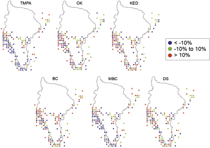
The spatial distribution of these scores across the study area reveals some insights into the relative per-formances between the merging methods. Figure 5

shows the percent bias, which is the ME normalized by the station average daily rainfall. MBC retains much of TMPA’s negative bias whereas DS improves along the Andes. This suggests that the latter has a better capa-bility for local correction, which is highly important for such a complex environment as the Andes. To a lesser extent, both methods also achieve correction in the lowlands, where the original TMPA is expected to al-ready perform well. Given OK’s tendency to converge to rain gauge measurements and that the meteorological FIG. 2. Annual mean precipitation of the TMPA, OK, and

merged products (1998–2008). The black line delimits the San Regis basin and the silver lines are country borders. The black dots indicate the locations of gauges used in the data merging. The Andean range follows the western boundary of the basin.

FIG. 3. The sensitivity analysis of BC’s variogram parameters performed on 10 Jan 1998. The figure shows (a) three different variogram parameterizations: (left) good model fit, (middle) overestimated range, and (right) underestimated sill; (b) the corresponding error variance field; and (c) merged products in comparison to the original (d) TMPA and BK fields.

evaluation takes rain gauge values as reference, OK performs well in general but in particular in the low-lands, and KED follows the same spatial pattern. This is also consistent with the expectation that spatial corre-lation is higher in the lowlands than it is in the

mountains. Moreover, OK and KED perform better in highly sampled regions, which is discernible inFig. 6in terms of higher modeling efficiency values at the centers of rain gauge clusters. Finally, this figure further suggests that the best merging products overall are achieved FIG. 4. Annual mean residual between merged products (including OK) and TMPA (1998–

2008). The black line delimits the San Regis basin and the silver lines are country borders. The black dots indicate the locations of gauges used in the data merging. The Andean range follows the western boundary of the basin.

using OK, KED, and DS. This is in spite of OK and KED’s poor representation of the spatial patterns of the annual mean precipitation over the entire merging field. This highlights another limitation of the meteorological cross-validation framework when applied to large areas with an uneven rain gauge density distribution.

c. Hydrological evaluation: Impact on the water balance and hydrological modeling at basin and subbasin scales

Table 3 presents a hydrological evaluation of the merging algorithms and shows several merging algo-rithms having a positive impact on the water balance. The most prominent improvements are seen with the DS, MBC, and (to a lesser degree) the KED methods in the upper Andean basins Borja and Santiago, where the runoff ratios are closer to the reference runoff ratio value of 0.7. In San Regis, the DS and MBC are similarly successful in reducing the water balance errors whereas KED increases them. In Chazuta, improvements are gained with the BC and DS methods, although the highest improvement in this subbasin is achieved with MBCS, which is an additional analysis that was run by excluding the rain gauges located outside the subbasin. In contrast, OK exacerbates the errors in all basins compared to TMPA.

The hydrological modeling results are summarized in terms of the performance scores across the basins.

Figure 7 shows RMSE and relative bias reductions as TABLE2. Performance scores from the cross validation of the

merging analysis calculated over 141 wet days between 1998 and 2008. The percent indicates a score relative to the TMPA score. The average precipitation intensity at the rain gauges is 10.3 mm day21_{. The best scores are in boldface.}

MAE RMSE _ME mm % mm % mm NSE TMPA 8.71 14.32 21.40 20.09 MBC 8.67 20.5 14.18 21.0 21.06 20.07 DS 8.18 26.1 13.03 29.0 0.10 0.09 OK 8.07 12.86 20.03 0.12 KED 7.95 28.7 12.62 211.9 0.09 0.15 BCR 8.86 11.7 14.82 13.5 20.36 20.17 BC 8.34 24.2 13.11 28.4 0.08 0.08

well as NSE increases (compared to TMPA) by MBC and DS, and additionally by BC in Chazuta subbasin. In contrast, OK, KED, and BC (except in Chazuta) show generally poorer scores for all four indices—percent bias, RMSE, correlation, and NSE—compared to TMPA. In Borja and Santiago subbasins, the DS method also resulted in above zero model efficiency. Over the entire modeled time series, the NSE improvements range from 0.1 to 0.5, with the higher increases achieved at Santiago and Borja.

4. Discussion and conclusions

The results of this case study suggest that the relative performances of the rainfall merging methods are strongly influenced by the rain gauge density over the domain of analysis. Overall, the DS method followed by the MBC method delivered the most consistent im-provement over the satellite product in both cross-validation and hydrological verification performance scores. Although the geostatistical methods, that is, KED and BC, did not result in a good hydrological performance, they nonetheless performed well in the

cross validation and showed the potential to produce valuable merged rainfall estimates if employed in suffi-ciently gauged areas. Finally, the underperformance of methods such as OK and KED in the hydrological evaluation, which either fully or heavily rely on rain gauge precipitation, supports the use of satellite-based products over gridded rain gauge products that utilize sparse data for hydrological modeling at large scales.

Guided by these observations, we propose inFig. 8a guideline for the selection of a merging method given FIG. 6. The NSE between merging product and rain gauge time series at all cross-validation points.

TABLE3. Spatial trends in the average runoff ratios calculated using observed streamflows and precipitation from gauge-adjusted TMPA. The expected value for humid tropical regions is between 0.6 and 0.7.

Regis Borja Santiago Chazuta

TMPA 0.66 0.98 1.33 0.79 MBC 0.63 0.96 1.28 0.81 DS 0.61 0.81 0.99 0.76 OK 0.85 1.04 1.35 0.87 KED 0.8 0.96 1.26 0.8 BC 0.74 0.97 1.45 0.75 MBCS 0.52 0.84 1.08 0.71

data characteristics and constraint and discuss this in the following.

The rain gauge network density in the studied basin should be considered when choosing the optimal merging method. In relatively well gauged basins (less than 250 km2 per gauge), the interpolation of gauge data only is believed to be sufficiently reliable for water resources applications (World Meteorological Organization 1994;Chappell et al. 2013), and simpler kriging methods such OK are regarded as accurate interpolation techniques for average daily rainfall (Collischonn et al. 2008;Buytaert et al. 2006a). How-ever, large-scale applications might violate the as-sumption of stationarity (a constant mean) in OK because of the nature of the spatial variability of pre-cipitation. KED provides a solution to this by in-troducing the external drift as observed by the satellite measurements.

In moderately gauged basins (between 250 and 1500 km2 per gauge), merging methods based on geo-statistics such as BC or KED provide valuable rainfall estimates, as demonstrated in the Chazuta subbasin. However, geostatistical methods may still be affected

by a number of practical limitations and fundamental assumptions. For example, the Gaussian distribution assumption made during the variance minimization in the weights estimation does not particularly hold for applications at fine temporal scale, as daily precipitation data are typically positively skewed, unlike monthly accumulations, which are more normally distributed. Ways around this problem are widely discussed in the literature, for example, through data transformation methods (e.g.,Müller 2007).

In poorly gauged basins (more than 1500 km2 per gauge), geostatistical merging methods have delivered unsatisfactory results because of a strong reliance on rain gauge observations over valuable satellite in-formation in ungauged areas. A possible cause could be the assumption of a known semivariogram common to all kriging estimators. Since the true semivariogram is unknown in reality, the experimental semivariogram is used instead in order to estimate the semivariogram parameters from the data. As far as rainfall fields are concerned, nonzero precipitation events tend to have a spatial footprint that negatively correlates to the intensity of the event (e.g., small-scale convective vs large-scale FIG. 7. Performance scores of daily streamflow using TMPA vs TMPA-gauge-adjusted products.

stratiform precipitation). This should be captured in the experimental semivariogram, but in poorly gauged ba-sins, distances between rain gauges are often too large and spatial correlation can be overestimated.

Instead, nonparametric merging methods DS and MBC have proved to be more robust to data scarcity. The success of the DS method reflects the spatial het-erogeneity of the climate and the size of the model field and supports the idea that distant gauges should have very little bearing on and should be given minimal weight in the estimation of unknown points simply based on their distance alone, particularly in very complex landscapes such as the Andean Amazon. A local cor-rection is best achieved by DS that substantially weights surrounding observed residuals by distance. MBC is attractive for its simplicity, but the assumption of a uniform multiplicative bias is a very narrow assumption given the complexity of the climate and the size of the domain. This is reflected by the improvements observed by applying the method to a smaller scale (with MBCSin Chazuta subbasin), which in essence is a move toward a more local bias correction. Extended methods such as

range-dependent mean bias correction have also been implemented in radar applications (e.g., Amitai et al. 2002) that can be adopted. The range threshold may further be made adaptable to the dominant precipitation processes (large-scale versus convective) in the area of the rain gauges.

This decision flowchart is intended to be a pre-liminary, nondefinitive guide to the selection of an op-timal method given the data characteristics. As it was developed based on experiences from a region charac-terized with highly heterogeneous topography and pre-cipitation processes, we expect this flowchart to hold for many other regions, at least for humid tropical and (sub) tropical mountain regions. Alternatively, an ensemble modeling approach can be considered that utilizes all of the merging inputs, whereby the model parameters can be weighted using Bayesian model averaging based on each model’s reproduction of observed streamflow (Jiang et al. 2012;Strauch et al. 2012).

Acknowledgments.Z.Z. and W.B. were funded by UK NERC Grant NE/I0040117/1 and NE-K010239-1. The authors thank Dr. Cinzia Mazzetti and Prof. Ezio Todini (University of Bologna) for making freely available to us the RAINMUSIC software package for meteoro-logical data processing.

REFERENCES

Almazroui, M., 2011: Calibration of TRMM rainfall climatology over Saudi Arabia during 1998–2009.Atmos. Res.,99, 400– 414, doi:10.1016/j.atmosres.2010.11.006.

Amitai, E., D. B. Wolff, D. A. Marks, and D. S. Silberstein, 2002: Radar rainfall estimation: Lessons learned from the NASA/ TRMM validation program.Proc. Second European Conf. on Radar Meteorology (ERAD), Delft, Netherlands, Delft University of Technology, 255–260.

Anagnostou, E. N., A. J. Negri, and R. F. Adler, 1999: Statistical adjustment of satellite microwave monthly rainfall estimates over Amazonia.J. Appl. Meteor.,38, 1590–1598, doi:10.1175/ 1520-0450(1999)038_,1590:SAOSMM_.2.0.CO;2.

——, V. Maggioni, E. I. Nikolopoulos, T. Meskele, F. Hossain, and A. Papadopoulos, 2010: Benchmarking high-resolution global satellite rainfall products to radar and rain-gauge rainfall es-timates.IEEE Trans. Geosci. Remote Sens.,48, 1667–1683, doi:10.1109/TGRS.2009.2034736.

Best, M. J., and Coauthors, 2011: The Joint UK Land Environment Simulator (JULES), model description—Part 1: Energy and water fluxes. Geosci. Model Dev., 4, 677–699, doi:10.5194/ gmd-4-677-2011.

Bookhagen, B., and M. R. Strecker, 2008: Orographic barriers, high-resolution TRMM rainfall, and relief variations along the eastern Andes.Geophys. Res. Lett.,35, L06403, doi:10.1029/ 2007GL032011.

Buytaert, W., R. Célleri, P. Willems, B. De Bièvre, and G. Wyseure, 2006a: Spatial and temporal rainfall variability in mountainous areas: A case study from the south Ecuadorian Andes.

J. Hydro.,329, 413–421, doi:10.1016/j.jhydrol.2006.02.031. FIG. 8. Decision flowchart for merging methods selection based on

——, V. Iniguezz, R. C_élleri, B. De Bi_èvre, G. Wyseure, and J. Deckers, 2006b: Analysis of the water balance of small Páramo catchments in south Ecuador.Environmental Role of Wetlands in Headwaters, NATO Science Series: IV, Vol. 63, Kluwer, 271–281, doi:10.1007/1-4020-4228-0_24.

Campling, P., A. Gobin, K. Beven, and J. Feyen, 2002: Rainfall– runoff modelling of a humid tropical catchment: The TOPMODEL approach. Hydrol. Processes, 16, 231–253, doi:10.1002/hyp.341.

Chappell, A., L. J. Renzullo, T. H. Raupach, and M. Haylock, 2013: Evaluating geostatistical methods of blending satellite and gauge data to estimate near real-time daily rainfall for Australia. J. Hydrol., 493, 105–114, doi:10.1016/ j.jhydrol.2013.04.024.

Collischonn, B., W. Collischonn, and C. E. M. Tucci, 2008: Daily hydrological modeling in the Amazon basin using TRMM rainfall estimates. J. Hydrol., 360, 207–216, doi:10.1016/ j.jhydrol.2008.07.032.

de Marsily, G., 1986: Quantitative Hydrogeology: Groundwater Hydrology for Engineers. Academic Press, 440 pp.

Deutsch, C. V., 1996: Correcting for negative weights in ordi-nary kriging. Comput. Geosci., 22, 765–773, doi:10.1016/ 0098-3004(96)00005-2.

Erdin, R., 2009: Combining rain gauge and radar measurements of a heavy precipitation event over Switzerland: Comparison of geostatistical methods and investigation of important influencing factors. Ph.D. thesis, ETH Zurich, 108 pp. Espinoza Villar, J. C., and Coauthors, 2009: Spatio-temporal

rainfall variability in the Amazon basin countries (Brazil, Peru, Bolivia, Colombia, and Ecuador).Int. J. Climatol.,29, 1574–1594, doi:10.1002/joc.1791.

Garreaud, R. D., M. Vuille, R. Compagnucci, and J. Marengo, 2009: Present-day South American climate.Palaeogeogr. Pa-laeoclimatol. Palaeoecol., 281, 180–195, doi:10.1016/ j.palaeo.2007.10.032.

Gjertsen, U., M.Sálek, and D. Michelson, 2004: Gauge adjustment of radar-based precipitation estimates in Europe.Proc. Third European Conf. on Radar Meteorology and Hydrology, Visby, Sweden, SMHI, ERAD, 7–11. [Available online at www. copernicus.org/erad/2004/online/ERAD04_P_7.pdf.] Goudenhoofdt, E., and L. Delobbe, 2009: Evaluation of

radar-gauge merging methods for quantitative precipitation esti-mates. Hydrol. Earth Syst. Sci., 13, 195–203, doi:10.5194/ hess-13-195-2009.

Grimes, D., E. Pardo-Iguzquiza, and R. Bonifacio, 1999: Optimal areal rainfall estimation using raingauges and satellite data.

J. Hydrol.,222, 93–108, doi:10.1016/S0022-1694(99)00092-X. Haberlandt, U., 2007: Geostatistical interpolation of hourly

pre-cipitation from rain gauges and radar for a large-scale extreme rainfall event. J. Hydrol., 332, 144–157, doi:10.1016/ j.jhydrol.2006.06.028.

Heidinger, H., C. Yarlequé, A. Posadas, and R. Quiroz, 2012: TRMM rainfall correction over the Andean Plateau using wavelet multi-resolution analysis. Int. J. Remote Sens., 33, 4583–4602, doi:10.1080/01431161.2011.652315.

Hewitt, A. J., 2012: Comparative assessment of gauge–radar merging techniques. Tech. Rep., Met Office, 9–19.

Huffman, G. J., and D. T. Bolvin, 2013: TRMM and other data precipitation data set documentation. Accessed 27 November 2013. [Available online at ftp://precip.gsfc.nasa.gov/pub/ trmmdocs/3B42_3B43_doc.pdf.]

——, and Coauthors, 1997: The Global Precipitation Climatology Project (GPCP) combined precipitation dataset.Bull. Amer.

Meteor. Soc.,78, 5–20, doi:10.1175/1520-0477(1997)078_,0005: TGPCPG.2.0.CO;2.

Jiang, S., L. Ren, Y. Hong, B. Yong, X. Yang, F. Yuan, and M. Ma, 2012: Comprehensive evaluation of multi-satellite pre-cipitation products with a dense rain gauge network and optimally merging their simulated hydrological flows using the Bayesian model averaging method.J. Hydrol.,452–453, 213–225, doi:10.1016/j.jhydrol.2012.05.055.

Kalman, R. E., 1960: A new approach to linear filtering and pre-diction problems.J. Basic Eng.,82(1), 35–45.

Kottek, M., and F. Rubel, 2008: Co-kriging global daily rain gauge and satellite data.Geophysical Research Abstracts, Vol. 10, Abstract EGU2008-A-03133. [Available online at http:// meetings.copernicus.org/www.cosis.net/abstracts/EGU2008/ 03133/EGU2008-A-03133.pdf.]

Krajewski, W. F., 1987: Cokriging radar-rainfall and rain gage data.

J. Geophys. Res.,92, 9571–9580, doi:10.1029/JD092iD08p09571. Lavado-Casimiro, W., D. Labat, J. L. Guyot, J. Ronchail, and J. J. Ordonez, 2009: TRMM rainfall data estimation over the Pe-ruvian Amazon–Andes basin and its assimilation into a monthly water balance model.IAHS Publ.,333, 245–252. Lehner, B., K. Verdin, and A. Jarvis, 2008: New global hydrography

derived from spaceborne elevation data. Eos, Trans. Amer. Geophys. Union,89, 93–94, doi:10.1029/2008EO100001. Li, M., and Q. Shao, 2010: An improved statistical approach to

merge satellite rainfall estimates and raingauge data.

J. Hydrol.,385, 51–64, doi:10.1016/j.jhydrol.2010.01.023. Maggioni, V., H. J. Vergara, E. N. Anagnostou, J. J. Gourley,

Y. Hong, and D. Stampoulis, 2013: Investigating the applica-bility of error correction ensembles of satellite rainfall prod-ucts in river flow simulations.J. Hydrometeor.,14, 1194–1211, doi:10.1175/JHM-D-12-074.1.

Mazzetti, C., and E. Todini, 2004: Combining raingages and radar precipitation measurements using a Bayesian approach.

geoENV IV—Geostatistics for Environmental Applications, X. Sanchez-Vila, J. Carrera, and J. J. Gómez-Hernández, Eds.,

Quantitative Geology and Geostatistics, Vol. 13, Springer, 401– 412, doi:10.1007/1-4020-2115-1_34.

Moore, R., B. Watson, D. Jones, and K. Black, 1989: London weather radar local calibration study: Final report. Rep. for the National Rivers Authority, Thames Region, NERC/ Institute of Hydrology, Wallingford, United Kingdom, 85 pp. Müller, H., 2007: Bayesian transgaussian kriging.Proc. 15th

Eu-ropean Young Statisticians Meeting, Castro Urdiales, Spain, Bernoulli Society, 5 pp.

PROGEA Srl, 2009: RAINMUSIC: Multi-sensor Bayesian com-binations. PROGEA Srl, Bologna, Italy, 119 pp. [Available online atftp://ftp2.progea.net/Web/RAINMUSIC_TechDoc_ ENG_2012.pdf.]

Rollenbeck, R., and D. Anhuf, 2007: Characteristics of the water and energy balance in an Amazonian lowland rainforest in Venezuela and the impact of the ENSO-cycle.J. Hydrol.,337, 377–390, doi:10.1016/j.jhydrol.2007.02.004.

——, and J. Bendix, 2011: Rainfall distribution in the Andes of southern Ecuador derived from blending weather radar data and meteorological field observations.Atmos. Res.,99, 277– 289, doi:10.1016/j.atmosres.2010.10.018.

Schiemann, R., R. Erdin, M. Willi, C. Frei, M. Berenguer, and D. Sempere-Torres, 2011: Geostatistical radar–raingauge combination with nonparametric correlograms: Method-ological considerations and application in Switzerland.

Hydrol. Earth Syst. Sci., 15, 1515–1536, doi:10.5194/ hess-15-1515-2011.

Silverman, B., 1998: Density Estimation for Statistics and Data Analysis.Monographs on Statistics and Applied Probability, Vol 26, Chapman & Hall, 175 pp.

Strauch, M., C. Bernhofer, S. Koide, M. Volk, C. Lorz, and F. Makeschin, 2012: Using precipitation data ensemble for uncertainty analysis in SWAT streamflow simulation.

J. Hydrol.,414–415, 413–424, doi:10.1016/j.jhydrol.2011.11.014. Tian, Y., C. D. Peters-Lidard, B. J. Choudhury, and M. Garcia, 2007: Multitemporal analysis of TRMM-based satellite precipitation products for land data assimilation applica-tions. J. Hydrometeor., 8, 1165–1183, doi:10.1175/ 2007JHM859.1.

Todini, E., 2001: A Bayesian technique for conditioning radar precipitation estimates to rain-gauge measurements.Hydrol. Earth Syst. Sci.,5, 187–199, doi:10.5194/hess-5-187-2001. Vila, D. A., L. G. G. de Goncalves, D. L. Toll, and J. R. Rozante,

2009: Statistical evaluation of combined daily gauge obser-vations and rainfall satellite estimates over continental South America.J. Hydrometeor.,10, 533–543, doi:10.1175/ 2008JHM1048.1.

Wang, L.-P., S. Ochoa-Rodr_íguez, N. E. Sim_ões, C. Onof, and C. Maksimovic, 2013: Radar–raingauge data combination techniques: A revision and analysis of their suitability for ur-ban hydrology.Water Sci. Technol.,68, 737–747, doi:10.2166/ wst.2013.300.

Wood, S., D. Jones, and R. Moore, 2000: Static and dynamic cali-bration of radar data for hydrological use.Hydrol. Earth Syst. Sci.,4, 545–554, doi:10.5194/hess-4-545-2000.

World Meteorological Organization, 1994: Guide to hydrological practices: Data acquisition and processing, analysis, fore-casting and other applications. WMO 168, 5th ed., 735 pp. [Available online atwww-cluster.bom.gov.au/hydro/wr/wmo/ guide_to_hydrological_practices/WMOENG.pdf.]

Yin, Z.-Y., X. Zhang, X. Liu, M. Colella, and X. Chen, 2008: An assessment of the biases of satellite rainfall estimates over the Tibetan Plateau and correction methods based on topo-graphic analysis. J. Hydrometeor., 9, 301–326, doi:10.1175/ 2007JHM903.1.

Zulkafli, Z., W. Buytaert, C. Onof, W. Lavado, and J. L. Guyot, 2013: A critical assessment of the JULES land surface model hydrology for humid tropical environments. Hydrol. Earth Syst. Sci.,17, 1113–1132, doi:10.5194/hess-17-1113-2013. ——, ——, ——, B. Manz, E. Tarnavsky, W. Lavado, and J.-L.

Guyot, 2014a: A comparative performance analysis of TRMM 3B42 (TMPA) versions 6 and 7 for hydrological applications over Andean–Amazon River basins.J. Hydrometeor.,15, 581– 592, doi:10.1175/JHM-D-13-094.1.

——, D. Nerini, and B. Manz, 2014b: Rainmerging: Pixel-point merging functions for precipitation time series. R package. [Available online athttps://github.com/zedzulkafli/Rainmerging.]