2013
A balanced approach to the multi-class imbalance
problem
Lawrence Mosley
Iowa State UniversityFollow this and additional works at:
https://lib.dr.iastate.edu/etd
Part of the
Operational Research Commons, and the
Statistics and Probability Commons
This Dissertation is brought to you for free and open access by the Iowa State University Capstones, Theses and Dissertations at Iowa State University Digital Repository. It has been accepted for inclusion in Graduate Theses and Dissertations by an authorized administrator of Iowa State University Digital Repository. For more information, please [email protected].
Recommended Citation
Mosley, Lawrence, "A balanced approach to the multi-class imbalance problem" (2013).Graduate Theses and Dissertations. 13537. https://lib.dr.iastate.edu/etd/13537
by
Lawrence Se’kou Denu Mosley
A dissertation submitted to the graduate faculty in partial fulfillment of the requirements for the degree of
DOCTOR OF PHILOSOPHY
Major: Industrial Engineering
Program of Study Committee:
Sigurdur ´Olafsson, Major Professor
Dianne Cook Stephen Gilbert
Heike Hofmann Lihzi Wang
Iowa State University Ames, Iowa
DEDICATION
TABLE OF CONTENTS
LIST OF TABLES . . . vi
LIST OF FIGURES . . . ix
ABSTRACT . . . xii
CHAPTER 1. INTRODUCTION . . . 1
1.1 Data Mining and the Operations Researcher . . . 1
1.2 A Gentle Introduction to Data Mining . . . 3
1.3 Supervised Learning in the Presence of Class Imbalance . . . 5
1.4 Thesis Structure . . . 7
CHAPTER 2. REVIEW OF LITERATURE AND BACKGROUND . . . 8
2.1 Supervised Learning . . . 8
2.1.1 Introduction . . . 8
2.1.2 Classification Models . . . 9
2.2 Model Assessment Metrics . . . 19
2.2.1 Model Validation . . . 19
2.2.2 Contingency Tables . . . 20
2.2.3 Two-Class Evaluation Measures . . . 21
2.2.4 k-Class Evaluation Measures . . . 23
2.3 Background and Formalization of the Class Imbalance Problem . . . 26
2.3.1 Formalization and Definitions . . . 26
2.3.2 Effects of Class Imbalance . . . 28
2.4 Current Approaches for Class Imbalance Prediction . . . 31
2.4.2 Algorithm Methods . . . 32
2.5 Data and Computing . . . 33
CHAPTER 3. A GLIMMER OF HOPE FOR MULTI-CLASS ACCURACY MEASUREMENT IN THE PRESENCE OF CLASS IMBALANCE . . . . 36
3.1 Introduction . . . 36
3.2 Definitions, Properties and Proofs . . . 39
3.2.1 Definition . . . 40
3.2.2 Interpretation and Proof . . . 42
3.2.3 Properties . . . 44
3.3 Calculation Examples . . . 49
3.4 On the Use of Class Balance Accuracy in Controlled and Uncontrolled Environ-ments . . . 54
3.4.1 Study 1: Initial Investigations into Class Balance Accuracy’s Practical Application . . . 54
3.4.2 Study 2: All-Red Boundary Tests . . . 59
3.4.3 Study 3: U.C.I. Hold-Out Study . . . 68
CHAPTER 4. MULTI-CLASS INSTANCE SELECTION WITH CLASS BAL-ANCE ACCURACY . . . 75
4.1 Introduction . . . 75
4.2 Background . . . 76
4.3 Study 1: Accuracy Comparisons between Class Balance Accuracy and Regular Accuracy Maximized Subsets . . . 77
4.4 Study 2: Accuracy Comparisons between Class Balance Accuracy and Regular Accuracy Maximized Subsets . . . 81
CHAPTER 5. A NOVEL APPROACH TO MODEL STACKING THROUGH CLASS EXPERT ENSEMBLING . . . 90
5.1 Introduction . . . 90
5.3 Algorithm . . . 91
5.4 Study: Investigation of Model Performance on Hold-Out Samples from the U.C.I. Model . . . 94
CHAPTER 6. TACKLING CLASS IMBALANCE WITH THE CLIMBR PACKAGE IN R . . . 103
6.1 Introduction . . . 103
6.2 climm: Class Imbalance Models and Measures . . . 106
6.3 climer: Class Imbalance Experts . . . 111
6.4 Utility Functions . . . 115
6.5 Package Expansion . . . 117
CHAPTER 7. CONCLUSION . . . 118
7.1 Future Extensions . . . 119
CHAPTER A. ADDITIONAL THEORY AND R IMPLEMENTATION . . . 120
LIST OF TABLES
Table 2.1 A 2x2 Confusion Matrix denoted asC2. . . 21
Table 2.2 Data set descriptions for the 16 data samples used in this research. . . 35
Table 3.1 A 3x3 Confusion Matrix denoted asC3. . . 41
Table 3.2 Invariance properties for performance criteria across binary and multi-class multi-classification tasks. Let “-” represent invariance, “∆” denote non-invariance and “±” highlight quasi-invariance. . . 48
Table 3.3 2x2 Confusion matrices highlighting the change in accuracies as minority or majority classes are correctly classified. . . 49
Table 3.4 Special case 3x3 confusion matrices without class imbalance where all cells are equal. . . 50
Table 3.5 Special case 3x3 confusion matrices without class imbalance where all observations have been predicted into one class. . . 50
Table 3.6 Special case 3x3 confusion matrices without class imbalance where each class has been perfectly classified. . . 51
Table 3.7 Special case 3x3 confusion matrices without class imbalance where one class is perfectly classified and all other observations have their labels switched by the classifier. . . 51
Table 3.8 Measure values calculated from Table 3.3 through Table 3.7. . . 51
Table 3.9 The majority class is perfectly predicted and no others. . . 53
Table 3.10 A minority class is perfectly predicted. . . 53
Table 3.12 Observations are assigned to classes based on the natural proportion of
the data. . . 54
Table 3.13 Multi-class measure values for each instance. . . 54
Table 3.14 Top performing models for each performance metric as assessed after training on the full Audio dataset. . . 55
Table 3.15 Top performing models for each performance metric as assessed after training on the full E. coli dataset. . . 56
Table 3.16 Per class recall for the E. coli dataset. . . 57
Table 3.17 Top performing models for each performance metric as assessed after training on the full Nursery dataset. . . 58
Table 3.18 Per class recall for the Nursery dataset. . . 58
Table 3.19 Measure rankings according to overall performance. . . 60
Table 3.20 Measure rankings according to per class performance. . . 61
Table 3.21 Hold out study results for the Anneal data set. . . 69
Table 3.22 Hold out study results for the Hepatitis data set. . . 71
Table 3.23 Hold out study results for the Page data set. . . 72
Table 3.24 Hold out study results for the Satellite data set. . . 73
Table 4.1 Instance selection model results from three simulated data sets. Three degrees of concept complexity were analyzed: Separable, Partially-Separable and Non-Separable. As the concept complexity increases, building mod-els from subsets that maximize Class Balance Accuracy will out preform similar subsets that maximize Regular Accuracy. . . 80
Table 4.2 Modeling results for the Diamonds data set per repetition by Instance Selection technique. . . 83
Table 4.3 Per class recall for the Diamonds data set per repetition by Instance Selection technique. . . 84
Table 4.4 Modeling results for the Glass data set per repetition by Instance Selec-tion technique. . . 87
Table 4.5 Per class recall for the Glass data set per repetition by Instance Selection technique. . . 88
Table 5.1 Model results ranked according to overall performance using Regular
Accuracy. . . 96
Table 5.2 Model results ranked according to per class performance using Class
Balance Accuracy. . . 98
Table 5.3 Modeling results for the Annealing data set. . . 99
Table 5.4 Per class recall for the Annealing data set. . . 100
Table 5.5 Class Expert choices for climer(CBA,CBA,DM) call on the Annealing
data set. . . 100
Table 5.6 Modeling results for the Balance Scale data set. . . 100
Table 5.7 Per class recall for the Balance Scale data set. . . 101
Table 5.8 Class Expert choices for climer(BA,OA,CP) call on the Balance Scale
data set. . . 101
Table 5.9 Modeling results for the Yeast data set. . . 101
Table 5.10 Per class recall for the Yeast data set. . . 102
LIST OF FIGURES
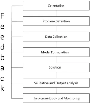
Figure 1.1 The Maynard’s Industrial Engineering Handbook visual representation
of the operations research approach. This work flow diagram describes
the steps necessary for systematic decision making and problem solving. 2
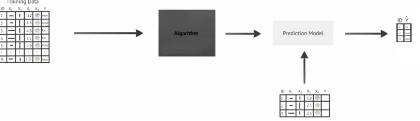
Figure 1.2 A process flow diagram of the supervised learning sequence. After the
data collection step, training data is used in conjunction with a machine learning algorithm to create a prediction model. This model can now be used to forecast class memberships of new, previously unforeseen
observations. . . 5
Figure 2.1 From left to right, the initial data is plotted and has it’s optimal
non-linear boundary derived by the classifier. The bounds are then used to differentiate between the two groups and here the accuracy of the bounds can be assessed. Lastly, the bounds themselves can be used to classify any data observation within the data space as either a red or
blue class member. . . 10
Figure 2.2 A decision tree with rules for differentiating between cereal
manufactur-ers based on a product’s sodium content, calories from fat, and weight per serving. . . 12
Figure 2.3 Random forest Gini based variable rankings for differentiating between
cereal manufacturers. . . 14
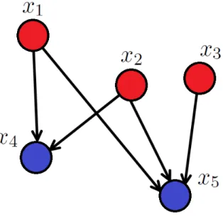
Figure 2.5 A network graph of connected events. The full joint probability can be given byp(x1∩x2∩x3∩x4∩x5) =p(x1)∗p(x2)∗p(x3)∗p(x4|x1x2)∗
p(x5|x1x2x3). . . 16
Figure 2.6 Sample linear and non-linear bound for a support vector machine. . . . 18
Figure 2.7 Multiple minority and multiple majority imbalance scenarios. . . 27
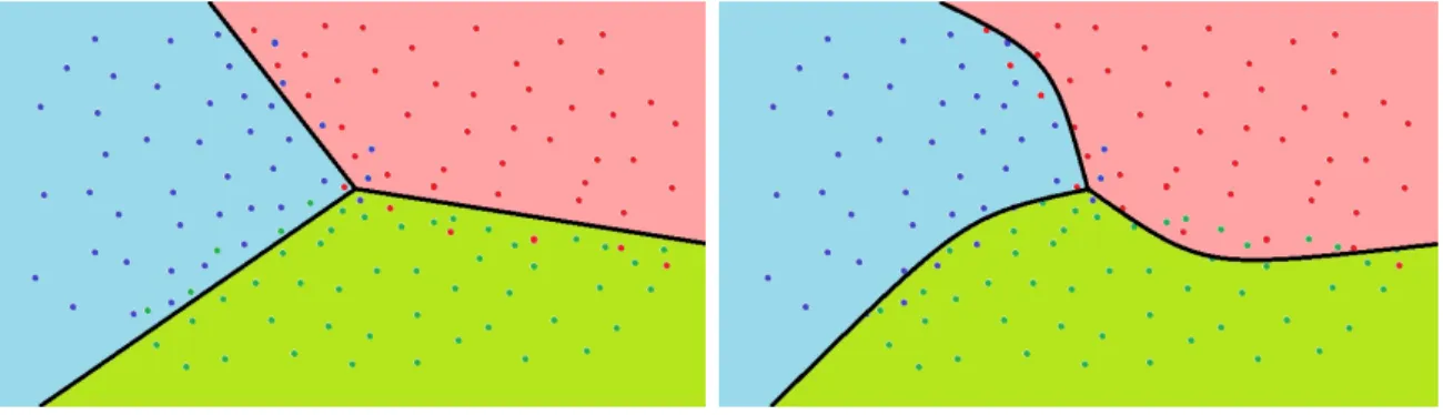
Figure 2.8 Both figures are suffering from concept complexity. On the left is a
dataset with small disjoints, while the figure on the right suffers from significant class overlap. . . 29
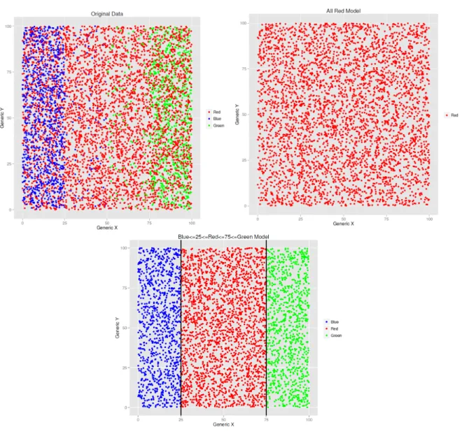
Figure 3.1 A data visualization of all red and class partitioned models derived from
the original data set on the top, left. Both models have the same level of accuracy, 62.5%, but clearly divide the data space differently. The Class Balance Accuracy for the all red and class partitioned models are
20.8% and 50% respectfully. . . 38
Figure 3.2 Values for five metrics across five matrices. CBA has the strongest
discriminancy ability, returning five distinct values, one for each matrix. 46
Figure 3.3 Data snapshot and convergence curves for two groups in a highly
sepa-rable scenario. . . 64
Figure 3.4 Data snapshot and convergence curves for two groups in a scenario with
average separability. . . 65
Figure 3.5 Data snapshot and convergence curves for two groups in a partially
separable scenario. . . 66
Figure 3.6 Data snapshot and convergence curves for two groups in a scenario with
low separability. . . 67
Figure 4.1 Modeling results for Instance Selection derived models after selecting a
subset that maximizes Class Balance Accuracy and one that maximizes
Figure 4.2 Modeling results for Instance Selection derived models after selecting a subset that maximizes Class Balance Accuracy and one that maximizes
Overall Accuracy under partially separable concept complexity. . . 79
Figure 4.3 A MDS plot of the full Diamonds data set. . . 85
Figure 4.4 Two MDS plots of the instances selected by maximizing CBA (top) and
Regular Accuracy (bottom) for iteration 1 on the Diamonds data set. . 86
Figure 4.5 A MDS plot of the full Glass data set. . . 88
Figure 4.6 Two MDS plots of the instances selected by maximizing CBA (left) and
Regular Accuracy (Right) for iteration 2 on the Glass data set. . . 89
ABSTRACT
The multi-class class-imbalance problem is a subset of supervised machine learning tasks where the classification variable of interest consists of three or more categories with unequal sample sizes. In the fields of manufacturing and business, common machine learning classifica-tion tasks such as failure mode, fraud, and threat detecclassifica-tion often exhibit class imbalance due to the infrequent occurrence of one or more event states. Though machine learning as a discipline is well established, the study of class imbalance with respect to multi-class learning does not yet have the same deep, rich history. In its current state, the class imbalance literature leverages the use of biased sampling and increasing model complexity to improve predictive performance, and while some have made advances, there are still no standard model evaluation criteria for which to compare their performance. In the presence of substantial multi-class distributional skew, of the model evaluation criteria that can scale beyond the binary case, many become invalid due to their over-emphasis on the majority class observations.
Going a step further, many of the evaluation criteria utilized in practice vary significantly across the class imbalance literature and so far no single measure has been able to galvanize consensus due not only to implementation complexity, but the existence of undesirable prop-erties. Therefore, the focus of this research is to introduce a new performance measure, Class Balance Accuracy, designed specifically for model validation in the presence of multi-class im-balance. This paper begins with the statement of definition for Class Balance Accuracy and provides an intuitive proof for its interpretation as a simultaneous lower bound for the average per class recall and average per class precision. Results from comparison studies show that models chosen by maximizing the training class balance accuracy consistently yield both high overall accuracy and per class recall on the test sets compared to the models chosen by other criteria. Simulation studies were then conducted to highlight specific scenarios where the use of class balance accuracy outperforms model selection based on regular accuracy. The measure is
then invoked in two novel applications, one as the maximization criteria in the instance selec-tion biased sampling technique and the other as a model selecselec-tion tool in a multiple classifier system prediction algorithm. In the case of instance selection, the use of class balance accuracy shows improvement over traditional accuracy in scenarios of multi-class class-imbalance data sets with low separability between the majority and minority classes. Likewise, the use of CBA in the multiple classifier system resulted in improved predictions over state of the art methods such as adaBoost for some of the U.C.I. machine learning repository test data sets. The paper
then concludes with a discussion of the climbRpackage, a repository of functions designed to
CHAPTER 1. INTRODUCTION
An introduction of data mining and its applications will be discussed as a build up towards our specific area of investigation. At that junction, research questions of interest will be estab-lished and a brief outline of the thesis structure will be given upon the chapter’s conclusion.
1.1 Data Mining and the Operations Researcher
Operations research as a discipline was built around the idea that analytical reasoning is the ideal method for evaluating alternatives. The process of selecting one alternative over an-other involves framing the problem as a highly structured mathematical program where the objective, decision variables, and constraints are made explicit and arranged in a manner that facilitates the search for optimal solutions. With this approach, agencies have been able to minimize costs, determine the best chemical proportions for gasoline blends, create the most efficient schedules, and find feasible fleet assignments across tens of thousands of variables and constraints (Rajgopal, 2001). The systematic organization of classical efficiency problems into solvable frameworks has been so successful that there is a common tautology now that em-phatically states “everything is an optimization problem”. As subscribers, we have no qualms about this statement’s truth. Regardless of our ability, or inability to solve these mathemati-cal programs, model formulation is only possible after a clear understanding of the objectives, inputs, and constraints. As a testament to its importance, industrial engineers have dedicated an entire step in the operations research work flow for this phase alone (Rajgopal, 2001). The “Data Collection” step in the operations research approach is designated as one such point in the work flow where relevant information is to be collected about the system, process, or event of interest. Data collected on subjects of interest serve to characterize the inputs with the hope
that later analysis will disclose important relationships between the characteristics. Questions
arise, Are certain geographical locations more prone to flight delays? Does the orientation of
the airport and the subsequent wind drift direction affect arrival times? Data driven solutions to these questions are used to form the basis for not only the decision variables and constraints of a program, but the inclusion or exclusion of parameters in the objective function, the key differential for solution discrimination. Therefore beyond simply collecting data for record keep-ing, there is a need to glean applicable knowledge from this information for the formulation of optimization problems.
Figure 1.1 The Maynard’s Industrial Engineering Handbook visual representation of the
op-erations research approach. This work flow diagram describes the steps necessary for systematic decision making and problem solving.
Sparked by human curiosity and made possible through human ingenuity, the data collec-tion process has become streamlined in such a way that it is now possible to record informacollec-tion across many subjects simultaneously and efficiently which increases the breadth of data. The volume of stored datum combined with the speed in which it is collected and the variety of
in-formation sources form the backbone of what industry has labeled “big data” (Stapleton, 2011). It becomes immediately apparent that to gain guiding insight from such large, high velocity data sets, the information contained must be processed in some automated fashion. It was this same desire for automation that inspired the machine learning scholars of yesteryear to develop the field of data mining to address the “big data” problems of their day (He, 2009). With an alternative paradigm to data analysis than traditional statistical thinking, data mining was introduced as a knowledge discovery tool that could, at the least, semi-automate the process of discovering previously unknown patterns in the data without an a priori hypothesis (Olafsson, 2008). The solutions to this insight search process are unknown patterns which can manifest themselves in two forms: as structured groupings of observations or relationships between in-put, output data fields. Standard nomenclature denotes the search for natural groupings as unsupervised learning tasks, whereas the investigation into relationships between explanatory variables and a labeled qualitative response is called supervised learning. Returning back to the operations research approach, given a domain context, the successful completion of these tasks can grant the industrial engineer valuable discernment into the model formulation. For
example, we may find thatanalysis suggests that both geographical location and runway
orienta-tion are related to traffic delays; therefore, these effects should be accounted for our formulaorienta-tion through the constraints, decision variables or objective function. Discussions of data mining thus far have revolved around its use in conjunction with the data collection step to aid indus-trial engineers in operations research tasks; however the applications of data mining can’t be constricted to one field. From the author’s own consulting experience data mining techniques have been sought after to differentiate between human and machine generated computer code, group graduate students according to post-baccalaureate school satisfaction, and analyze online text reviews of hotels for specific areas of competitive advantage.
1.2 A Gentle Introduction to Data Mining
Beyond general applications, for the purpose of this thesis, a more in depth discussion of data mining is warranted. As mentioned previously, data mining tasks exist in two realms, where
the learning process is either supervised and unsupervised. Unsupervised learning tasks aim to gather observations into clusters, where the ideal outcome involves the formulation of groups of observations with similar characteristics. In this scenario, the machine learning algorithm uses the input data and subsequently the underlying data structure to determine the optimal cluster membership for each case. This specific type of learning process can also be viewed as a search for latent variables within the data structure, where both the location and number of groups are unknown. Despite having objective data to guide the learning process, there is no way to verify that the clusters drafted by the algorithm are indeed veritable, which lends credence to state-ment that these techniques are “learning without a teacher” (Tibshirani and Freedman, 2009). That said, practitioners often calculate measures which describe the cluster’s compactness and separability; two intuitive measures that quantify the within cluster distances between obser-vations and the between cluster distances, respectfully (Grira, 2005). Based on these measures, a successful unsupervised learning task will create clusters that minimize the within-cluster distances while simultaneously maximizing the between-cluster distances, resulting in clusters that are tightly knit and spread apart. Popular algorithms include the distance based methods like k-means and hierarchical clustering, and self-organizing maps which were derived from the theory of topological maps (Tibshirani and Freedman, 2009). Common applications of unsu-pervised learning involve market segmentation of customers, grouping of countries with similar to economic output, and signal categorization.
Supervised learning differs from unsupervised learning because well-defined class labels ex-ist for each observation. Given a set of characterex-istics for the observations, amongst them the corresponding class label, classification models sift through the noise in the data set and output relevant relationships between the characteristics and the class labels. Some of these relationships can be expressed as intuitive patterns, like“after 5 pm the risk of a network log-in being malicious increases two fold” or “ip addresses that attempt to log-in more than 10 times at perfectly space intervals are 75% more likely to be machines compromised with a Trojan virus than other client terminals”. To attain these rules, the first step is to partition the data into training and test sets that contain 66.6% and 33.3% of the data, respectfully. With the training set, a model is learned and classification rules are created. These newly developed
classification rules are applied to the test data to assess the accuracy and robustness of the model on observations outside of the original training set. This emulates model usage in the real world. To determine the model’s level of accuracy, for each observation in the test set, predictions are derived from the model rule set and are compared with its true class observed from the data. The sum of the number of observations whose predicted class and observed class match are divided by the total number of observations in the data set, which results in high predictive accuracy for models that can recall more of the original observed class labels. This ability to assess the model, as a consequence of having known class memberships, supervises the learning process. As the more formalized branch of machine learning, its uses are pervasive in all branches of science with broad, diverse applications too numerous to list. A survey of
applications can be found in Tibshirani and Freedman’s“Elements of Statistical Learning”.
Figure 1.2 A process flow diagram of the supervised learning sequence. After the data
collec-tion step, training data is used in conjunccollec-tion with a machine learning algorithm to create a prediction model. This model can now be used to forecast class mem-berships of new, previously unforeseen observations.
1.3 Supervised Learning in the Presence of Class Imbalance
Supervised learning models are widely applicable and can offer substantial insights into how the explanatory variables are related to the categorical response variable. The ability of
models to discover useful patterns in data rely on some key assumptions that provide justifi-cation for the use of statistical machine learning methods. One such assumption is that there is an underlying deterministic mechanism that generates differences between the groups. This assumption clearly disallows the possibility that the class labels are a sole result of chance. Another fundamental assumption, and the main topic of this thesis, is the requirement that all levels of the categorical outcome variable be evenly distributed. Deviations from this assump-tion are exhibited when the one of more levels of the response variable are not represented at the same relative frequency as the other levels. This scenario is aptly named, the class imbal-ance problem (Japkowicz, 2000). Since all classification models seek to find boundaries between classes, in cases where there is a departure from this assumption, meaningful boundaries are hard to ascertain. Reduced to its core, class imbalance makes the very act of prediction more difficult because of the added challenge to group delineation and demarcation (Longadge et. al, 2013). Aside from the added difficulty of partitioning the data space, when the target variable has skewed class distributions, the fundamental intuition behind performance accounting is attacked as imbalance increases. In these situations, performing assessment begins to transi-tion from straight forward ratio calculatransi-tions and branches into the realm of informatransi-tion theory and matrix reduction. Classifiers are implicitly or explicitly designed to segment the classes to optimize the total number of correctly specified observations. When the objective is merely to maximize the number of observations, classifiers manifest a myopic view of the task which guides them toward the prediction of classes that are over represented in the data set (Kumar and Sheshadri, 2012). As an example, given ninety-eight observations with “positive” labels, a single “negative” observation, and a single “neutral” labeled instance, if the latter two points are not conspicuously separated in the data space then most classifiers would be well suited to create a rule that classifies all observations as a positive group member. The learning rule would achieve ninety-eight percent accuracy, but effectively provide no new knowledge if the initial objective was to gain insight and demarcate boundary lines between the three classes. While the value added of this classification model would be nil, our evaluation criteria returns a value that suggests directly the opposite. In effect, when information about each class is inte-gral, class imbalance severely hinders the effectiveness of traditional accuracy as a performance
measure. This dissertation acknowledges these short comings and seeks to address the class imbalance problem by introducing a novel alternative measure for model evaluation, one that balances the precision and recall metrics across each class.
1.4 Thesis Structure
In this chapter we have discussed how data mining serves as a central part of the modern
operations research work flow. An overview of supervising and unsupervised learning was
presented, as well as an introduction to the class imbalance problem along with a discussion of its effect on model evaluation. The remainder of this PhD thesis will be outlined in the following sequence.
In chapter 2, we will review the background and literature relevant to the class imbalance problem. It will begin with a formalization of supervised learning tasks within the context of class imbalance. The class imbalance problem will be revisited, including an in-depth discussion of its effects and current approaches. The chapter will conclude with supplemental discussions on material relevant to work done in subsequent chapters. Chapter 3 will begin with a formal proposal of the Class Balance Accuracy measure. Sections will be devoted to its definition, proofs, properties, intuition, and a concluding comparison study highlighting its use as a model evaluation criterion in practice. Where relevant, simulation studies will be discussed to provide additional experimental evidence in support of the measure. In Chapters 4 and 5, two novel applications of class balance accuracy are introduced. In both, Class Balance Accuracy is used within the objective function, where in one the goal is to determine the selection of subsets for instance selection and in the other to determine suitable class experts for a multiple
classifier system. Simulation studies for each method are conducted to show how the use
of our proposed measure can improve accuracy in the presence of non-separable multi-class data sets. Afterward, Chapter 6 will walk through a software implementation of the methods and procedures introduced to address the class imbalance problem. The chapter will provide interactive documentation for the use of functions specifically designed to assist with model prediction and evaluation in the presence of class imbalance. In conclusion, the final chapter will summarize the key points of this PhD research and discuss future extensions.
CHAPTER 2. REVIEW OF LITERATURE AND BACKGROUND
It is the intent of this chapter is to give the reader a sufficient background understanding of the class imbalance problem and knowledge of the current state of the art.
2.1 Supervised Learning 2.1.1 Introduction
Let a m-dimensional vector of measurements be denoted by X, where each dimension is
identified as xj such that j = 1,...,m. In conjunction, let Y be a singleton element from the
setG, that contains, k, elements distinguished asg1,g2,gj,...gk. Combined, the 2-tuple{X,Y}
form one complete data observation. A n-dimensional collection of these data observations,
{X,Y}n, form the completedataset from which classification models are trained.
The supervised learning process consists of a structured search through the data space by
a chosen member a subset of models within, M, the superset of all available models. For
any given model, say Ml, when trained with some randomly selected subset of data,
classifica-tion boundaries are drawn based on the locaclassifica-tion of optimal separaclassifica-tions that maximize some algorithm based measure of separation (Tibshirani and Freedman, 2009). Commonly used as-sessments of separation are Kullback-Leibler divergence and the Gini coefficient. Boundaries derived from these models may consist of rule based criteria that delineate the classes according to the values of the input variables or archetypal observations that serve as threshold limits where all observations more extreme are deemed to be from another group extant in the data. Due to the diversity of algorithm approaches for boundary detection, there can be a reasonable expectation for a commensurate amount of heterogeneity in model interpretability. Generally, as models increase in complexity, the effects of the explanatory variables are no longer
extri-cable due to the lack of closed form partitionable formulas. Ideally, to preserve the individual input variable effects, their contribution should be structured in such a manner that facilitates easy differentiation, not unlike the concept of partitioning sum of squares in the linear model framework (Kutner et.al, 2004). Interpretability aside, these boundaries established by the models are used for the prediction of observations with complete records across all explanatory variables, regardless of the existence of pre-observed class labels. Predictions are given as ˆYi,
corresponding to the ith observation’s prediction, where every label forecast is one of the
pos-sible groups contained inG. Intuitively, after the original data space has been demarcated, it
then degenerates leaving only the model derived boundaries as marker fields or zones. Each zone corresponds to a specified label, wherein all observations contained within are classified into the boundary specified group. Hence, at the conclusion of the supervised learning process, the training data has been used to calibrate the model which results in estimated boundaries for the various classes.
2.1.2 Classification Models
Statistical procedures and machine learning algorithms that perform supervised learning tasks are aptly called classifiers. As a collective unit, classifiers each perform the same duties, transforming input data into class membership predictions, yet individually, each technique is grounded in theory derived from different assumptions and hypothesis. The work involved in this thesis will revolve around six standard classification models: Classification and Regression Trees, Random Forests, AdaBoost, Naive Bayes, Support Vector Machines, and Neural Net-works. To establish a rudimentary understanding of the models and their approaches, a brief introduction to each classifier will be provided. It is the intent of the introduction to familiarize the reader with the theoretical underpinnings of each technique and highlight the diversity in methodology.
F igur e 2. 1 F rom le ft to righ t, the in it ial d at a is pl ot te d and h as it ’s op ti m al non -l in ear b oun d -ar y d er iv ed b y th e clas si fi er . Th e b ou n ds ar e th en us ed to d iff er en ti ate b et w ee n th e tw o gr oup s and h er e the acc ur ac y of the b oun ds can b e ass es se d. Last ly , th e b oun ds th ems el v es ca n b e us ed to cl ass if y an y d at a obs er v at ion wi th in the d at a sp ace as eit h er a red or bl u e cl as s me m b er .
2.1.2.1 Classification and Regression Trees
Decision tree learning is all encompassing phrase that describes rule based partitioning methods. Developed in the early 1980’s, classification and regression trees, like most machine learning algorithms, had its usefulness spurned by the advent of high-powered, low cost com-puting. These rule based techniques rely on the identification of homogenous “splits” derived from subsetting along regions of the input variables (Tibshirani and Freedman, 2009). The dual process of feature selection and split construction are the initial phases in the tree algorithm design. Determining the variable order involves searching among the explanatory variables for fields that will yield the most homogenous splits. A split’s quality is assessed through vari-ety of metrics which can include information gain or entropy calculations (Ripley et.al, 2013). Through the use of impurity metrics, each split’s level of homogeneity can be quantified. As candidate fields are selected and included in the tree, the rule-based model grows, encompassing a large yet nuanced path along the data space. Because it is a split-based partitioning method, classification and regression trees paths can be easily interpreted. Each path represents a given a set of scenarios that lead to a cluster of similar observations. Following along each path, the model accounts for interactions between variables within the data space. As such, classification trees are an excellent tool for the search of interactions between fields with the inside of an exploratory data analysis framework. Recursive partitioning techniques, do not have any set assumptions that must be followed. That said, the lack of assumptions to be explicitly satisfied does not grant liberty from careful consideration to the application. As a result of the algo-rithm’s construction, variables with a larger number of categories are preferred over variables with fewer levels and when the model is allowed to grow in an unconstrained fashion, the prob-lem of overfitting cannot be avoided. The phenomenon of overfitting occurs when the model grows and complexity and reaches the point where the given data can be perfectly explained by the model yet the complexity mars its ability to make generalized predictions (Izenman, 2008). To protect against the scenarios machine learning practitioners take careful consideration to examine the resulting rules from the tree algorithm. Moreover, to combat the overfitting issue, pruning techniques have been developed that impose penalties for excessive growth beyond
essential branches. Despite its relative simplicity, tree-based methods have been proven to be a reliable and largely attainable technique for model based prediction (Tibshirani and Freedman, 2009).
Figure 2.2 A decision tree with rules for differentiating between cereal manufacturers based
on a product’s sodium content, calories from fat, and weight per serving.
2.1.2.2 Random Forests
Machine learning experts, borrowing from the field of statistics, realized that improvements to tree based predictions could be easily accomplished by incorporating resampling methods, in conjunction with model ensemble techniques, into the modeling framework (Breiman, 2001). This simple modification increased the computational costs and complexity of the modeling procedure, yet has been shown to increase predictive accuracy while maintaining resistance
to overfitting. Dubbed, random forests, the algorithm gained notoriety after Leo Breiman’s seminal paper where he described the process of randomly selecting from a fixed training set and allowing only a subset of variables to act as candidates to entry. The algorithm forms a random subspace wherefore features are searched through. As a result of the randomization of both the features and the subset, diversity is induced within the subsequent trees that are created. This process is akin to taking small randomly selected subsections of data along with random subsets of features, fitting a tree model to each subset, and repeating the procedure
a predefined number of times. More formally, for some subset of training objects, N and
fea-tures, X, at each iteration choose a subset x of size |x| to be the number of input variables
to be used in each individual classifier such that |x| < |X|. Select |M| to be the number of individual classifiers to be fit by the ensemble. For each classifier, m, we first randomly sample
|N| observations from the data, with replacement, and fit a tree classifier without any growth
constraints. Each model is given a single vote and the majority voting scheme is employed to determine the class membership of each observation.
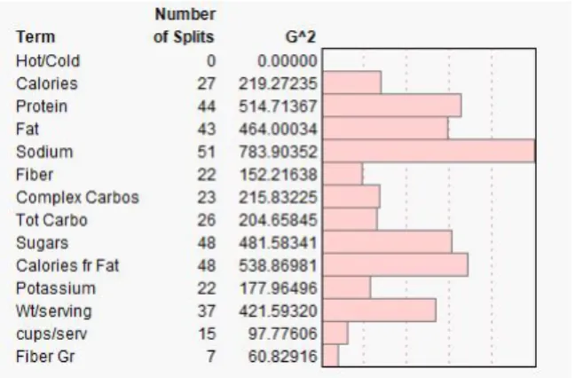
Random forests have been shown to be not only efficient on larger datasets, but also out-perform other more sophisticated machine learning techniques (Breiman, 2001). Other benefits of random forests include the lack of a need for cross validating the model to develop an un-biased estimate of test set error and the ability of the model to return Gini based variable importance rankings, along with a host of features that are documented in Breiman’s original paper. Practitioners have been well served by the variable rankings returned by the random forest procedure. They are a natural result of the tree based construction, are not limited to only categorical or continuous variable types. To accomplish its variable importance ranking, the decrease in Gini for splits under each tree is summed across all trees in the forest and sorted according to the variables which have the largest decrease in Gini. Further advances in the ideas of model aggregation, resampling and computation have spurned even more state of the art techniques that rest on the same fundamental principles as random forests. One such advancement has been the advent of adaptive boosting which will be discussed in the next section.
Figure 2.3 Random forest Gini based variable rankings for differentiating between cereal man-ufacturers.
2.1.2.3 AdaBoost
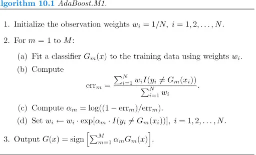
Boosting is a machine learning approach that supposes the use of many “weaker” models, i.e. low preforming classifiers, crowd sourced to create a single well-informed body of classifiers that will improve predictions by accounting for the collective experience of the group (Freund, 1997). This concept is not unlike the random forest procedure, but is generalized to apply to techniques beyond just classification and regression trees. At the crux, boosting provides a systematic framework for fitting multiple classifiers, reweighting their value according to performance on individual observations. Though the previous statement may imply that the classifiers themselves are being reweighted, within the actual algorithm, the observations are
assigned an initial weight, say wi = 1/N. Each observation unsuccessfully classified has its
weight reinitialized before the next model fit. Key to the final predictions is the majority vote formula: G(x) =sign( M X m=1 αmGmx) (2.1)
The function G(x) serves as an aggregator for the individual predictions of each classifier. Figure 2.4 shows the Adaboost.M1 procedure as described by Tibsherani, Fredman and Hastie
on page 339 ofThe Elements of Statistical Learning.
Figure 2.4 The Adaboost.M1 algorithm procedure.
Lastly, the authors show that the AdaBoost algorithm reduces to the optimization of an additive model across an exponential loss function where solutions are found through the use of a gradient descent search procedure. As a result of the gradient descent technique and the structure of the problem, it has been shown that random classification noise can have a negative effective on AdaBoost’s performance. None withstanding, AdaBoost methods perform well in practice and give comparable results with other ensemble based methods (Tibshirani and Freedman, 2009).
2.1.2.4 Naive Bayes
Probabilistic graphical models are relatively simple techniques that allow for the visual ac-counting of probability augmented characterizations of networked events. These interconnected events have their stochastic properties modeled through the use of conditionally independent probabilities. This allows for the use of complex computations to be expressed and calculated within the graph theory framework. An even more simplistic version of this technique,
specif-ically applied to supervised learning, is the Naive Bayes classifier. As its name suggests, the naive Bayes classifier is grounded in probability theory with Bayes rule at the crux.
Figure 2.5 A network graph of connected events. The full joint probability can be given by
p(x1∩x2∩x3∩x4∩x5) =p(x1)∗p(x2)∗p(x3)∗p(x4|x1x2)∗p(x5|x1x2x3).
Bayes rule allows for the estimation of conditional probabilities not directly observed using information that can be directly measured and quantified. Under the independence assumption, Naive Bayes classifiers exploit the factorization property the independence structure grants to calculate conditional and joint probabilities of class memberships. Satisfaction of the indepen-dence assumption also imposes a ‘naivety” assertion that gives equal weight to all features used in the model. This has the unfortunate side effect of making Bayes classifiers susceptible to increased signal noise caused by irrelevant features which may hinder performance (Rish and Watson, 2009). Executing the Naive Bayes classification scheme requires the computation of the maximum a posteriori decision rule which is calculated by selecting the class that yields the largest posterior probability.
Class(x1, . . . , xm) = argmax g p(G=g) m Y i=1 p(Xi=xi|G=g) (2.2)
The above equation quantifies the choice of class as the group membership that maximizes the posterior probability as calculated by looking at the conditional probability of a feature given a specific class. True to its Bayesian nature, the prior information is contained in the
p(G = g) term obtained from the observed class memberships in the data. Applying the
product across each of these observed conditional probabilities ranks the posteriors with respect to the class of interest so that the one with the highest value can be selected. It has been shown in the past that deviations from the independence assumption makes the numerical estimates unreliable, but do not lead to permutations in the rankings of posterior probabilities and therefore the final output, an estimated class membership, are often reliable predictions. Due to its simplicity and efficiency, the Naive Bayes classifier even has an Apache Mahout big data implementation that works for gigabyte and terabyte sized datasets (Rish and Watson, 2009).
2.1.2.5 Support Vector Machines
Hermann Minikowski, a German mathematician, is responsible for creating the “separating hyperplane theorem”. This theorem purports that if given two disjoint, closed, convex sets,
say A and B, with properties such that one set is compact, then these two sets have a pair
of points p and q where one point lies in each set such that a hyperplane exists perpendicular to the line segment between points p and q. Minikowski’s assertion shows that under certain conditions there will exist an N-dimensional line segment that will separate convex sets. In ma-chine learning, the exact conditions do not hold for every set, but the concept of searching for a separating hyperplane motivated the creation of a technique called support vector machines. This technique involves finding a solution to a quadratic programming problem of the form:
minw,b 12kwk2
yi(w·x−b)≥1
Where w is a normalizing vector, b is a constant, x is the value of the observation, and
y is the class of the observation. This quadratic program can be relaxed with Lagrangian
multipliers to make the problem more tractable. In practice, most boundaries between classes are not separable due to overlap, which hinders the search for a support bound that maximizes the distance between the support vectors. This can be compounded with the addition of non-linear boundaries. To account for this scenario, what is known as a “kernel trick” can be applied to the data by recasting the datum into a higher dimension and searching for a linear bound. When the data is returned to its original dimension, the resulting higher dimensional linear bound is now non-linear. This powerful and clever mathematical transformation has proven to be extremely useful in practice (Tibshirani and Freedman, 2009). Support vector machines have been shown to preform very well in practice for both binary and multi-class prediction problems.
Figure 2.6 Sample linear and non-linear bound for a support vector machine.
2.1.2.6 Neural Networks
Originating to emulate the biochemistry of the brain, neural networks is one of the most popular machine learning algorithms in use today. As a model, it attempts to focus on linear combinations of the inputs and then characterize the response variable as a function of these
yet as it was studied in more detail some of its short-comings became more apparent. Neural networks have an inability to handle mixed data well, have no integrated procedure for handling missingness, can be biased easily due to outliers, do not scale well, aren’t interpretable and do not handle noisy input variables with any degree of intelligence (Arel, 2010). Beyond those shortcomings, neural networks also have a tendency to overfit to the existing training data (Kotsiantis, 2007). As a result, the ubiquitous use of neural networks waned toward the end of the 1990’s due to issues with its performance. Recently, big data repositories and extensions of neural networks aptly named “deep learning” has brought on a resurgence of the technique’s popularity. When given a sufficient amount of data, neural networks ability to model nuances allows for the quick search through large feature spaces for patterns that traditionally not be distinguishable. Within small data contexts, these same patterns often serve as noise, yet with sufficient data these patterns give marginal improvements in accuracy which can be substantial in the aggregate. Deep learning algorithms attempt to improve predictions by layering neural network models into a machine that conceptualizes a hierarchy of features in the data (Arel, 2010).
2.2 Model Assessment Metrics 2.2.1 Model Validation
Model evaluation is crucial to the machine learning, data mining process because it is the method by which the legitimacy of models are tested. As such an important phase in the learning process, the evaluation must be simultaneously both objective and robust. To fulfill the objectivity necessity, quantitative measures, be they information-theoretic based or matrix reduction, are used to provide a singular numerical representation of the quality of a model. Representing this model quality with error or misclassification rates is standard, just as well as citing their inverse, accuracy. Scenarios with imbalance will be discussed later; however, performing model evaluation for multi-class problems is not just a straightforward extension of the binary case. Many techniques do not have multi-class extensions, particularly ones set in an information theoretic frame. Therefore any measure utilized in a multi-class situation
must be robust beyond the binary case. The following sections will introduce commonly used metrics and discuss their use in practice.
2.2.2 Contingency Tables
The consortium of performance measures defined on 2x2 confusion matrices and their more
generalkxkcounter parts can be parsed based on how the off diagonal misclassification
knowl-edge is processed (Wei et.al, 2010). Measures derived from information theory treat the actual class as a model input and their corresponding predictions as output. The classifier, acting as a communication channel between input and output, allows for the use of information theoretic tools which seek to characterize the amount of entropy or information loss in a given confusion matrix (Moreno and Albacete, 2010). In essence, the confusion matrix is acting as a random variable and its information content measured accordingly. These measures usually afford a high degree of matrix discrimination, which serves well to detect differences in misclassification rates from similar matrices, an asset when class distributions are skewed in favor of one class. Unfortunately the nature of information theoretic derivations, which rely heavily on non-trivial differential entropy, make extensions of these measures difficult to construct as supported anec-dotally by their scarcity in the multi-class prediction assessment literature. The other branches of measures rely on confusion matrix reduction and transformation to glean misclassification information (Moreno and Albacete, 2010). Individual elements and sums are manipulated to
reduce thektimeskmatrix entries into a single number that represents the classification
accu-racy. This simplicity often comes with a cost, as information loss is inevitable when reducing
a kxk table into a single number (Chauvin et.al, 2000).
We will briefly discuss the some of the more common measures applied to two-class and
k-class prediction. Let Ck denote a confusion matrix or the contingency table of actual class
labels by their model predictions, with cij representing the number of cases with true label i
Predicted
Class 1 Class 2 Total
Actual Class 1 c11 c12 c11 +c12
Class 2 c21 c22 c21 +c22
Total c11 +c21 c12 +c22 N
Table 2.1 A 2x2 Confusion Matrix denoted asC2.
2.2.3 Two-Class Evaluation Measures
AccuracyAs the current de-facto accuracy measure, overall Accuracy is simple to calculate and interpret. Within a contingency table, successfully classified observations appear along the
diagonal. Accuracy, therefore, is simply the proportion of correctly classified observations
divided by the total number. Following the notation in Table 2.1, Accuracy is defined as:
Accuracy= c11+c22 c11+c12+c21+c22
(2.3) Recall, Precision, and the F-measure Despite being easily attainable, this 3-tuple of measures is less commonly used. As per Table 2.1, classifier Recall is calculated from the number of correct Class 1 matches divided by the total number of actual Class 1 cases. Similarly, Precision aptly describes how precise a model is by dividing the number of correct Class 1 matches by the total number of predicted Class 1 instances. The F-measure supplements them by reducing both measures into a single number by producing the harmonic mean between Precision and Recall. The usefulness of these measures has largely been restricted to document retrieval and similar applications. Their formula is as follows:
P recision= c11 c11+c21 (2.4a) Recall= c11 c11+c12 (2.4b) F−measure= 2∗Recall∗P recision
Recall+P recision (2.4c)
Sensitivity and Specificity Reporting the sensitivity and specificity of a laboratory di-agnostic test is a generally accepted practice in the medical literature because of their direct
relation to type I and type II error. Sensitivity is identical to the Recall measure discussed erst-while and is calculated for Class 1. Specificity judges a classifier’s ability to correctly identify Class 2 instances. To avoid misleading conclusions, both numbers are reported when assessing testing procedures. At this time, aside from averaging across each class, no well-established multi-class generalization exists. Explicitly stated the formulas for Sensitivity and Specificity are: Sensitivity = c11 c11+c12 (2.5a) Specif icity= c22 c21+c22 (2.5b)
ROC and AUC Receiver Operator Characteristic (ROC) curves and the Area Under the Curve (AUC) are common measures in medicine, machine learning, and a host of other fields (Arun and Sheshadri, 2012) that want to take advantage of the well behaved statistical prop-erties and leverage the graphical nature of the technique. Unlike the previously mentioned techniques, ROC curves are not defined on a single confusion matrix but on the class probabil-ity estimates. In combination with the probabilprobabil-ity estimates, if given a set probabilprobabil-ity threshold value, a model’s sensitivity can be plotted on the y-axis against the false positive rate creating the curve. Naturally, the area under the curve could serve as a measure of model quality, since at perfect accuracy both ROC axis measures are maximized suggesting that larger areas are superior. This single number reduction has prompted hopeful researchers to seek meaningful multi-class extensions of the AUC measure. One such extension, the Volume under the Surface, has been derived but was shown to be particularly unwieldy (Moreno and Albacete, 2010). It wasn’t until Hand’s work in 2009 did the entire foundation of using AUC as a measure become suspect. Hand boldly states that “...using the AUC is equivalent to using different metrics to evaluate different classification rules.” Recently other authors have cited his work and published extensions or proposed their own alternative solutions for AUC’s incoherency.
2.2.4 k-Class Evaluation Measures
Matthew’s Correlation CoefficientFirst introduced in 1975 by Brian W. Matthews for
the 2x2 case, this measure has been carefully studied and shown to have connections to the χ2
distribution (Chauvin et.al, 2000). The measure has some other notable characteristics, such as an intuitive [-1,1] range where the bounds represent perfect misclassification and perfect classification, respectively. MCC calculates a value of 0 for confusion matrices that indicate the classifier preformed the classification randomly. Findings have discussed MCC’s relationship with Confusion Entropy, a measure discussed later, have been explored for fruitful results (Jurman and Furlanello, 2010). Though MCC has been gaining more traction as one of the best binary classification task measures, how it performs in multi-class settings with unbalanced groups has not yet been well studied. The formal expression is as follows:
M CC = k P i,l,m=1 ciicml−clicim v u u t n P k=1 ( n P k=1 clk)( k P f,g=1 f6=k cgf) v u u t k P i=1 ( k P i=1 cil)( k P f,g=1 f6=k cf g) (2.6)
Relative Classifier Information RCI is an information theoretic approach designed ex-pressly to summarize how distinctly classes have been demarcated (Wei et.al, 2010). This measure has a deceptively intuitive range of [0,1] where large values indicate better classifica-tion performance; however, the measure’s construcclassifica-tion does not account for actual accuracy
only the uniformity of the predicted classes. Stated explicitly, the formula for RCI is given as: RCI = Hc Hd (2.7a) Hd=− n X i=1 n P i=1 cil n log( n P i=1 cil n ) (2.7b) Ho = n X j=1 n P k=1 ckj n Hoj (2.7c) Hoj =− n X i=1 cij n P k=1 ckj log( ncij P k=1 ckj ) (2.7d) Hc=Hd−Ho (2.7e)
Confusion Entropy Continuing within the information theory framework, Wei et.al. de-fine their measure, Confusion Entropy, on multi-class confusion matrices by focusing on all available information contained in the off diagonal entries. As a result of their careful deriva-tion, they created a measure that discriminates among matrices better than any previous mea-sure to date (Jurman and Furlanello, 2010). The resolution of Confusion Entropy’s separations is so pronounced that the measure values can’t assign a unique value to all cases that represent random classification like its MCC counterpart. For this entropy measure, small values repre-sent less information loss and better classification, and in practice this fact must be kept in the forefront because of its counterintuitive nature. The Confusion Entropy is defined as:
CEN = n X j=1 Pj X k=1 k6=j h2(n−1)(Pjkj ) +h2(n−1)(Pkjj ) (2.8a)
hb =P(x)logb(P(x)) (2.8b) Pijj = n cij P k=1 cjk+ckj (2.8c) Piji = n cij P k=1 cik+cki (2.8d) Pj ij = n P k=1 cjk+ckj 2 n P k,l=1 ckl (2.8e) Piii = 0 (2.8f)
Balanced Accuracy Balanced Accuracy is the Recall for each class, averaged over the number of classes. As an assessment tool it is intuitively simple, the predictive quality is measured for each class independently and aggregated. Balance accuracy derives all of its information from the diagonal elements and the row sums.
Balanced Accuracy= c11 c11+c12 + c22 c21+c22 2 (2.9) (2.10) G-Mean Similar to Balanced Accuracy, the Geometric Mean focuses only on the Recall of each class. What differentiates this measure from balance accuracy comes from the way the class recall is aggregated; multiplicatively instead of additively across each class.
G−M ean= (Πi=1ri) 1
k (2.11a)
ri =Recall f or Group i (2.11b)
The multi-class measures show much more promise than their 2x2 counterparts with regards to practical application in the presence of imbalance, yet the field is still open for measures that can provide simplicity, are mathematically coherent and extendable beyond two classes.
2.3 Background and Formalization of the Class Imbalance Problem In this section the class imbalance problem will be formalized and followed with a discussion of its effects on supervised learning tasks.
2.3.1 Formalization and Definitions
Suppose for a given dataset, {X,Y}n, we recall that the Yncomponent is an-dimensional
collection of singleton elements from the set G, whose units are distinct labels g1,...,gk. Here
we introduce the set P, a container for the proportions of each class distribution. In similar
fashion to the erstwhile defined sets, the elements of P are denoted asp1,p2,pj,...pk. Each pk proportion has a value that ranges from 0 to 1.
Classical machine learning algorithms assume the response variable has an equal number of observations within each class. The multi-class imbalance problem can be stated simply as
any deviation from this assumption where at least one class proportion pi is not equal to the
other proportions when k >2. It is obvious that in practice, most if not all tasks will exhibit imbalance due to the inability to control the outcome of a model, experiment or procedure. It is true however, that since data mining tasks involve the development of the model ex post some procedure, and it is possible to select an equal number of observations of each class as long as the researcher is comfortable ignoring observations. Imbalance can also occur in instances where limitations are due to collection of data due to cost or privacy. Returning to our previous thought, class imbalance, according to its strict definition, occurs frequently in practice, and yet does not have much effect on the outcome unless the imbalance reaches some threshold. Unfortunately, it is at this junction where the objectivism of defining class imbalance departs. Because imbalance can occur at varying degrees, there is no set standard wherefore we can definitively say that the imbalance within a class variable is indeed a problem. Currently, at best we can hope for the development of a threshold value that will indicate if a response subset suffers from class imbalance to such a degree that it will have some impact on the modeling process (Japkowicz, 2000). At this point in time there is no such indicator.
publica-tions have established definipublica-tions for two common imbalance scenarios (Wang and Yao, 2012). For any multi-class problem, a “multi-minority” case is one where a single class has a signif-icantly larger proportion than the average size of all other classes. The converse situation is where a single class has a significantly smaller proportion than the average size of all classes. This is deemed the “multi-majority” case. This situation can be formalized aspmin<< pwhere
p is the average proportion across all classes. Likewise for the multi-minority case pmaj >> p
wherep (Wang and Yao, 2012).
Figure 2.7 Multiple minority and multiple majority imbalance scenarios.
Wang and contributing authors point out that both forms of imbalance negatively affect both overall and per class performance. They found that multi-majority cases to be the more harmful of the two, hindering common data based imbalance solutions, ultimately leading to overfitting issues. In addition, when multiple minority classes exist, random undersampling greatly reduced the majority class performance. In the next section we will discuss the effects of class imbalance in more detail.
2.3.2 Effects of Class Imbalance
Class imbalance influences data mining tasks by proxy. In the presence of imbalance, algo-rithms can be initialized, their procedure will run, and converge can be met; therefore, the effect of imbalance are largely symptomatic. Despite a non-terminal prognosis for models trained un-der imbalanced distributions, unequal class distributions exacerbate already troublesome data mining issues such as over-shadowing minority classes when there exists concept complexity, introducing additional training bias when building models with a small sample sizes, and in-validating commonly used accuracy measures (Japkowicz, 2000).
2.3.2.1 Concept Complexity
When majority and minority classes exhibit a low amount of separability within the feature space, the data is said to express a high degree of concept complexity. The idea of separability communicates the degree in which observations share similar values along fields in the feature space. With each similar value, learning techniques must search an alternative variable or linear combination of fields to separate the observations. In the presence of imbalance, this overlap creates blurred boundaries between the classes (Drummond and Holte, 2005). When combined with an accuracy driven algorithm, it creates a situation where the minority class observations can be ignored (Drummond and Holte, 2005; Wang and Yao, 2012; Dongre and Malik, 2013). This will be a critical theme within this body of work.
As a generalized term, concept complexity also describes the linearity of the class bound-aries. Linearly separable boundaries are the holy grail of modeling bounds. Nearly all algo-rithms, either search based or statistically grounded, can find an optimal linearly separable plane where groups can be partitioned (Tibshirani and Freedman, 2009). These bound also happen to be easily interpretable with explanations that are conducive to creating classification rules. Unfortunately, when bounds are non-linear, the “classification bounds” for groups can take any shape or form, which increases the computational effort required to carve boundaries to some sensible approximation. A further complication can occur when these clusters of mi-nority observations do not reside in one centralize location within the data space. Scattered
pockets of disjoint minority classes can exist with non-linear bounds and in situations where the overlap of majority classes seep into the minority class segments algorithms err towards ignoring the minority class segments (Wang and Yao, 2012).
Figure 2.8 Both figures are suffering from concept complexity. On the left is a dataset with
small disjoints, while the figure on the right suffers from significant class overlap.
2.3.2.2 Small and Noisy Data
Noisy data can be described as data that have been gathered in some ill-prepared manner, incorrectly labeled, or contain features that provide spurious information. Minority class ob-servations, which already exhibit sparse representation, are especially prone to noise by biasing the boundaries away from their true limits. As a consequence of noise, classes that originally may be linearly separable now increase in concept complexity and bring along with it all the subsequent ramifications (Garcia et.al, 2007).
It is intuitive that the fewer data points in the datum, the easier it is to separate groups, the faster algorithms will converge and higher the likelihood for the boundaries to be linearly separable; however, as a consequence of having a reduced sample sizes, group demarcations found will not be generalizable. With imbalance extant, the metes created to differentiate the
minority class observations may not approximate the true boundaries because of sampling bias.
2.3.2.3 Evaluation
As discussed previously, model evaluation is an integral part of the data mining process. When comparing and contrasting the model predicted class memberships with the actual class groupings any measure utilized should consider both the overall accuracy of predictions along with the individual class recalls. In the presence of imbalance, accuracy measures that focus on overall performance will have a tendency to ignore minority classes because as a group they do not contribute much to the general performance (Zeno et.al, 2011). As a classic example, given ninety-eight observations with “positive” labels, a single “negative” observation, and a single “neutral” labeled instance, if the latter two points are not conspicuously separated in the data space then most classifiers would be well suited to create a rule that classifies all observations as a positive group member. The learning rule would achieve ninety-eight percent accuracy, but effectively provide no new knowledge if the initial objective was to gain insight and demarcate boundary lines between the three classes. While the value added of this classification model would be nil, our evaluation criteria returns a value that suggests directly the opposite. In effect, when information about each class is integral, class imbalance severely hinders the effectiveness of traditional accuracy as a performance measure.
Unfortunately, it is still common practice for scholars to report measures that account only
for the overall performance of the classifier (Galar et.al, 2012). This is a result of a lack
of consensus for the choice of measures in the presence of skewed class distributions. Many measures lack the ability to be generalized to the multi-class case, which hinders their use beyond binary classification and therefore are invalid for multi-class imbalance problems. As a further consequence of complexity, implementations of non-matrix reduction techniques are uncommon and restricted to a few programming languages. Therefore there is a gap in the literature for any measure that can account for accuracy across all classes, is robust to the cardinality of the class set, and possesses a form that is easily implementable.
2.4 Current Approaches for Class Imbalance Prediction
Previous investigations into imbalance have shown that the effects of skewed class distribu-tions are a function of the degree of imbalance, the amount of overlap between the minority and majority classes, the overall size of the data and the classifier itself (Wang and Yao, 2012; Japkowicz, 2000). Methods to address class imbalance attempt to do so by mitigating the in-fluence of one of those four characteristics of the modeling process. These characteristics form the basis for the two general approaches that involve either data space manipulation, algorithm modifications or an amalgamation of both. This section we will discuss common approaches to the class imbalance problem in more detail.
2.4.1 Data Methods
A straight-forward procedure involves rebalancing the class distributions through resam-pling the data space. These methods involve either oversamresam-pling the minority class or under-sampling the majority class. In their simplest form, overunder-sampling and under under-sampling involve the random selection of data observations already extant in the data. This has the consequence of being computationally quick, however both can potentially and often do bias the datum in unintentional ways. Oversampling the minority class has been known to increase the chances of overfitting because observations within the minority class are exact replicas of one another. Random undersampling does not have this effect, but can potentially discard useful obser-vations. To account for the shortcomings, techniques such as synthetic minority oversampling technique and selective preprocessing of imbalance data were introduced. SMOTE is a k-nearest neighbor approach to minority class oversampling. The hope is that the overfitting problem can be sidestepped by generating new instances from a random interpolation of existing minority members. SPIDER is a hybrid technique that involves both over sampling the minority class and under sampling the majority class through an intelligent two-phase process of identifica-tion and preprocessing. The first phase begins with the identificaidentifica-tion of misclassified instances using k-nearest neighbors. The second phase then decides whether to amplify minority class instances, amplify the minority class instances and relabel majority class instances, or just