IMPROVING THE COMPUTATIONAL EFFICIENCY
OF APPROXIMATE DYNAMIC PROGRAMMING
USING NEURAL NETWORKS, WITH APPLICATION
TO A MULTI-RESERVOIR HYDROPOWER AND WIND
POWER SYSTEM
A Dissertation
Presented to the Faculty of the Graduate School of Cornell University
in Partial Fulfillment of the Requirements for the Degree of Doctor of Philosophy
by
Kyle Robert Perline December 2017
c
2017 Kyle Robert Perline ALL RIGHTS RESERVED
IMPROVING THE COMPUTATIONAL EFFICIENCY OF APPROXIMATE DYNAMIC PROGRAMMING USING NEURAL NETWORKS, WITH APPLICATION TO A MULTI-RESERVOIR HYDROPOWER AND WIND
POWER SYSTEM Kyle Robert Perline, Ph.D.
Cornell University 2017
This dissertation develops a more computationally efficient Approximate Dy-namic Programming (ADP) method that can be applied to optimal control prob-lems that are stochastic, nonconvex, and either finite or rolling horizon with many stages. The primary application is to a realistic model of Bonneville Power Ad-ministration, which is a large wind power and hydropower producer in the Pacific Northwest. The objective is to determine the optimal amount of power to buy and sell on the day and hour ahead markets conditioned on the wind power forecast, as well as how much water to release from each reservoir.
The second Chapter in this dissertation develops the Fitting via Unimodal Ap-proximation Optimization (FUA) method for more accurately approximating the value function in ADP with a Feedforward Neural Network with one hidden layer (FFNN1). A major part of FUA is the new Unimodal Approximation Optimization (UAO) algorithm that is used to perform FFNN1 hyperparameter optimization. UAO can be applied to optimization problems with a discrete domain and a noisy unimodal objective function, and it is proven that UAO converges almost surely to the correct solution. Results on two control problems with 4, 12 and 15 state space dimensions show that approximating the value function in ADP with an FFNN1 using FUA yields a more accurate control solution in less time as compared to
using other methods of fitting an FFNN1.
Chapter 3 presents the Long Term Generation method that generates long-term synthetic wind power scenarios conditioned on historical sequential short-term wind power forecasts. Power systems with wind power integration can be simulated on this data in order to more accurately evaluate the performance of their control policies. Additionally, the Joint Distribution Comparison test is developed to evaluate the quality of these synthetic scenarios.
Finally, in Chapter 4 a stochastic rolling horizon model of Bonneville Power Administration is developed and the resulting control problem is solved using the ADP algorithm developed in Chapter 2 and is evaluated using data generated in Chapter 3. The stochastic control formulation has a nonlinear objective function, 24 decision variables, and 16 state space dimensions.
BIOGRAPHICAL SKETCH
Kyle Perline was born in Burlington, Vermont on October 24, 1989 to Kevin Perline and Lori Rippa. Kyle has always had a love of mathematics, engineering, and physics, which led him to attend the Honors Program at Clarkson University from 2008 to 2012. There, he obtained a double Bachelor of Science Degree in Physics and Mathematics, as well as a double Bachelor of Science Degree in Aeronautical Engineering and Mechanical Engineering. In the summer of 2012 Kyle first went to Cornell and began work with his adviser Christine Shoemaker.
ACKNOWLEDGEMENTS
Thank you to my adviser Christine Shoemaker. Throughout five and a half years she helped me focus my research and yet gave me enough flexibility to explore my changing interests.
I am grateful to the entire Center for Applied Mathematics. This includes all of the staff, directors, and in particular my committee members, Alexander Vladimirsky and Huseyin Topaloglu, who help make CAM an excellent academic program. Of course, my time there was so enjoyable largely because of my fellow CAM students, and I thank all of them for giving me motivation to go to the office. I would also like to thank everyone I worked with during my internship at The Aerospace Corporation during the Spring of 2016.
Finally, I want to share my appreciation for my entire family.
This work was supported by the National Science Foundation Grant DGE-1650441, the Center for Applied Mathematics, and teaching assistantships in Cor-nell’s Mathematics Department.
TABLE OF CONTENTS
Biographical Sketch . . . iii
Dedication . . . iv Acknowledgements . . . v Table of Contents . . . vi List of Tables . . . ix List of Figures . . . xi 1 Introduction 1 Bibliography 7 2 Improved Stochastic Neuro-Dynamic Programming with Appli-cations to Hydropower 9 2.1 Abstract . . . 10
2.2 Introduction . . . 10
2.3 Background on Feed Forward Neural Networks and Research Plan . 15 2.3.1 Component C1: Training Algorithms ES and BR . . . 17
2.3.2 Component C2: Generalization Error Estimation methods TSM and VSM . . . 18
2.3.3 Component C3: Hyperparameter Optimization algorithms UAO, BO, G, R . . . 18
2.3.4 Component C4: Ensemble . . . 19
2.3.5 Summary: F it(C1, C2, C3, C4) . . . 19
2.3.6 Implementation . . . 20
2.4 Fitting with Unimodal Approximation Optimization . . . 21
2.4.1 Unimodal Approximation Optimization Algorithm . . . 25
2.4.2 UAO Theoretical Considerations and Convergence . . . 29
2.4.3 Comparison of Hyperparameter Optimization Algorithms and Error Estimation Methods . . . 31
2.5 Test Problems . . . 37
2.5.1 4D Hydropower . . . 37
2.5.2 12D Hydropower . . . 37
2.5.3 15D Inventory . . . 40
2.6 Comparing FFNN1 Fitting Algorithms on ADP Test Problems . . . 41
2.7 Conclusions . . . 48
2.A FFNN1 Training Error Distribution Plots . . . 49
2.B Theoretical Properties of the Unimodal Approximation Optimiza-tion Algorithm . . . 53
2.B.1 Proof of Lemma 1 . . . 53
2.B.2 Proof of Bounded θ . . . 54
2.B.3 Proof of Convergence Theorem . . . 56
2.D Speedup Definition . . . 73
2.E Computation and Accuracy Analysis Trials . . . 75
2.F Computation Time Plots . . . 77
Bibliography 79 3 Generating Long-Term Wind Scenarios Conditioned on Sequen-tial Short-Term Forecasts 83 3.1 Abstract . . . 84
3.2 Nomenclature . . . 84
3.3 Introduction . . . 85
3.4 Notation . . . 90
3.5 Long Term Generation Method . . . 91
3.5.1 Handling Missing Historical Data . . . 95
3.5.2 Existing Evaluation Methods . . . 97
3.6 Joint Distribution Comparison . . . 98
3.6.1 Application of JDC on Simulated Data . . . 101
3.7 Computational Results . . . 111
3.7.1 Naive Concatenation Method . . . 111
3.7.2 Bonneville Power Administration Dataset . . . 112
3.7.3 Results . . . 113
3.8 Note on Optimized Covariance Parameter . . . 121
3.9 Conclusions . . . 125
Bibliography 127 4 Operation of Wind and Hydropower Producer With Market In-fluence 131 4.1 Abstract . . . 132
4.2 Introduction . . . 132
4.3 Wind and Hydropower Producer Model . . . 135
4.3.1 Reservoir State Dynamics and Constraints . . . 136
4.3.2 Hydropower Generation . . . 140
4.3.3 Wind Power Forecasts and Scenarios . . . 142
4.3.4 Combined Model Price Functions . . . 144
4.3.5 Individual Model Price Functions . . . 147
4.4 Rolling Horizon Control Formulation . . . 149
4.4.1 Decision Variables . . . 150
4.4.2 State Space . . . 151
4.4.3 State Transition . . . 152
4.4.4 Benefit Function . . . 153
4.4.5 Dynamic Programming Equation . . . 154
4.4.6 Neuro-Dynamic Programming Solution . . . 155
4.5 Results . . . 157
4.5.1 Finite Horizon Convergence . . . 158
4.5.2 Comparison of Combined and Individual Models . . . 159
4.5.3 Comparison of Varying Market Influence . . . 164
4.6 Conclusions . . . 168
4.A Terminal Value Function . . . 170
Bibliography 177
LIST OF TABLES
2.1 Component 3 speedup results — values greater than one means UAO is faster. Speedups Serror
U AO-C2,C3-C2(t) shown in bold boxes compare F it(ES, C2, C3,1), with Component C2 denoted by su-perscript (b) and C3 denoted by (a), to F it(ES, C2, U AO,1) on 9 test problems denoted byc. If C2=TSM thenerror is test set error, if C2=VSM then error is validation set error. For example, con-sider the top left bolded 3X2 box, where the number in the first row and first column is 2.00. This indicates that on test problem 4D-16 (4D is on the left side of the row, L=16 is on the top of the column) the fitting algorithm F it(ES, V SM, BO,1) (BO is on the left side of the row, VSM is on the top of the column) required 2.00∗12 = 24 seconds of computation time (wheret = 12 seconds is on the top of the row) to obtain a mean estimated error not statistically larger than what the fitting algorithm F it(ES, V SM, U AO,1) obtained in 12 seconds. . . 35 2.2 Component 2 speedup results — values greater than one means
VSM is better than TSM. Speedups SL2
C3-V SM,C3-T SM(t) compare
F it(ES, V SM, C3,1), with Component C3 denoted by superscript (a), toF it(ES, T SM, C3,1) on 9 test problems denoted byc. Com-parison uses L2 error of trained FFNN1 with smallest estimated error. For example, consider the top left number in the table, which is > 2. This indicates that in the test problem 4D-16 (4D and L = 16 are both on top of the row) the fitting algorithm
F it(ES, T SM, U AO,1) (algorithm UAO is on the left side of the row) required (> 2)∗25 = (> 50) seconds of computation time (t = 25 seconds is shown on the top of the column) to obtain a mean L2 error not statistically larger than what the fitting algo-rithm F it(ES, V SM, U AO,1) obtained in t= 25 seconds. . . 36 3.1 Seven variations of Long-Term Generation method. . . 91 3.2 Determining the ability of the JDC test to identify if a perturbed
distribution is biased and/or scaled for different values ofK. Larger z-scores, defined in Equation (3.25), indicate the JDC test can more reliably distinguish when samples are drawn from different distri-butions. . . 110 3.3 Three variations of Naive Concatenation Method. . . 112 3.4 Brier Scores. Bold are best scores, underlined are worst scores. . . 118 3.5 Historical variance of errors (first row), optimized exponential
co-variance parameter (second row), and first derivative of coco-variance function (third row). . . 124 4.1 Reservoir release constraints, measured in ksfd/8 hours. . . 139
4.2 Operational hydropower reservoir volume constraints, measured in ksfd. Numbers in parentheses are absolute reservoir bounds. . . 139 4.3 Run-of-river reservoir volume bounds, measured in ksfd. . . 139 4.4 Square root of mean hourly squared error (MWh) between power
sold in the full dynamic programming and simplified models. . . . 163 4.5 Summary statistics of the Combined and Individual Models . . . . 166
LIST OF FIGURES
2.1 Distribution of estimated generalization errorsXhD,C2 when training an FFNN1 with h hidden nodes and using Early Stopping. The solid lines show the 95% confidence interval of the estimated mean on the domain H = {1,2, ...,100}, and the dashed line shows the mean. The boxplots show the distribution for h= 1,5,10, ...,100. 22 2.2 Progress plots comparing optimization algorithms applied to
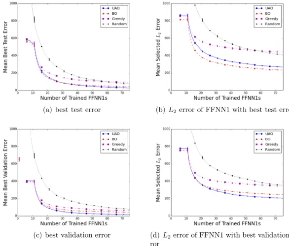
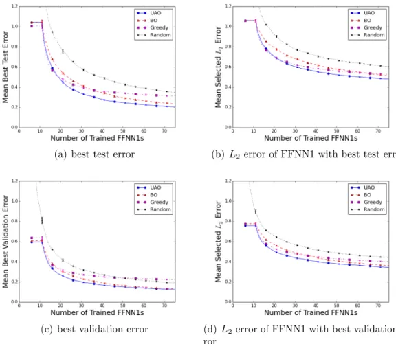
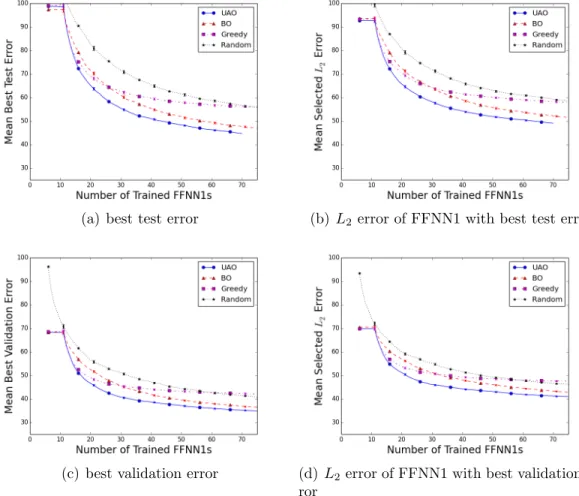
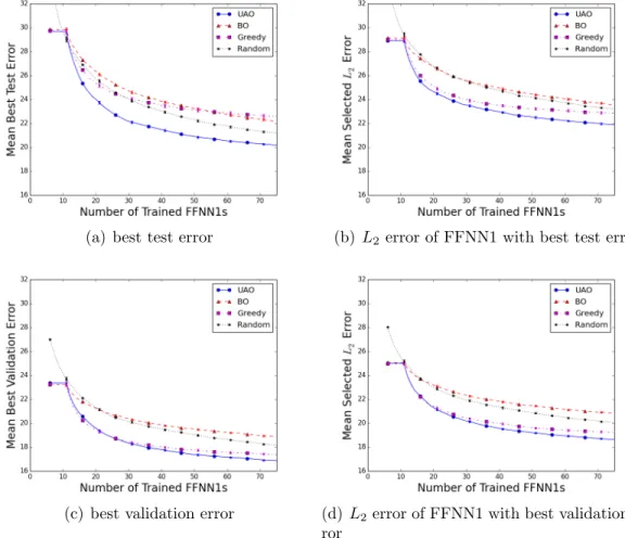
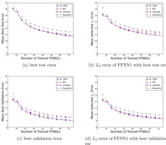
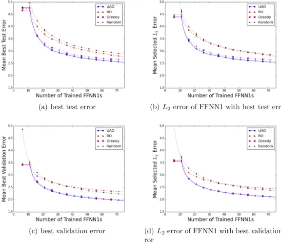
dataset 12D-750, i.e. the dataset from the 12D Hydropower prob-lem withL= 750; top plots use Component C2=TSM, bottom use C2=VSM. Plots show mean performance over 1,000 trials, error-bars show standard deviation of estimate of the mean and are often too small to be seen. . . 32 2.3 Visual explanation of speedup comparisonSA,Berror(t). Ssolid,dashederror (t0) =
Serror
dashed,solid(t0) = 1 (algorithms same), Sdashed,soliderror (t1) = t2/t1 > 1 (dashed is better), Serror
solid,dashed(t2) =t1/t2 <1 (solid is worse) . . . . 34 2.4 Reservoir network diagram. Numbers indicate the reservoir
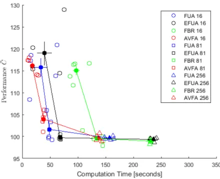
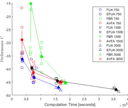
num-ber. Gray reservoirs have water capacity and white reservoirs are run-of-the-river. Water enters the system through reservoirs 1, 2, and 3. . . 39 2.5 Computation and Accuracy Analysis in plots (a)-(c). Some BR
data points have MEC values too large (bad) to fit on the plot. Plot (d) shows computation time of the 12D Hydropower problem. Black bars are training time, white bars are time to evaluate state space samples, and bar height is total time. . . 44 2.6 Statistical Accuracy Analysis. An ‘X’ indicates the column test
case statistically outperforms the row test case at the 5% level, an ‘O’ is the reverse, and an empty square indicates no statistical difference. . . 47 2.7 FFNN1 error distributions in 4D Hydropower problem. The solid
lines show the 95% confidence interval of the estimated mean on the domain H = {1,2, ...,100}, and the dashed line shows the mean. The boxplots show the distribution on domainH={1,5,10, ...,100}. 50 2.8 FFNN1 error distributions in 12D Hydropower problem. The solid
lines show the 95% confidence interval of the estimated mean on the domain H = {1,2, ...,100}, and the dashed line shows the mean. The boxplots show the distribution on domainH={1,5,10, ...,100}. 51 2.9 FFNN1 error distributions in 15D Inventory problem. The solid
lines show the 95% confidence interval of the estimated mean on the domainH={1,2, ...,100}, and the dashed line shows the mean. The boxplots show the distribution on domainH={1,5,10, ...,100}. 52 2.10 Progress plots comparing optimization algorithms applied to test
2.11 Progress plots comparing optimization algorithms applied to test problem 4D-81. . . 65 2.12 Progress plots comparing optimization algorithms applied to test
problem 4D-256. . . 66 2.13 Progress plots comparing optimization algorithms applied to test
problem 12D-750. . . 67 2.14 Progress plots comparing optimization algorithms applied to test
problem 12D-1500. . . 68 2.15 Progress plots comparing optimization algorithms applied to test
problem 12D-3000. . . 69 2.16 Progress plots comparing optimization algorithms applied to test
problem 15D-750. . . 70 2.17 Progress plots comparing optimization algorithms applied to test
problem 15D-1500. . . 71 2.18 Progress plots comparing optimization algorithms applied to test
problem 15D-3000. . . 72 2.19 Computation and Accuracy Analysis for the 4D Hydropower test
control problem. . . 75 2.20 Computation and Accuracy Analysis for the 12D Hydropower test
control problem. Some BR data points have MEC values too large (bad) to fit on the plot. . . 76 2.21 Computation and Accuracy Analysis for the 15D Inventory test
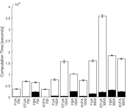
control problem. Some BR data points have MEC values too large (bad) to fit on the plot. . . 76 2.22 Computation time of the 4D Hydropower problem. Black bars are
training time, white bars are time to evaluate state space samples, and bar height is total time. . . 77 2.23 Computation time of the 12D Hydropower problem. Black bars are
training time, white bars are time to evaluate state space samples, and bar height is total time. . . 78 2.24 Computation time of the 15D Inventory problem. Black bars are
training time, white bars are time to evaluate state space samples, and bar height is total time. . . 78 3.1 Qualitatively showing the simulated distributions (b) and (c) are
similar to the historical BPA data set (a). . . 102 3.2 Examining the impact of increasing the number of scenariosNS on
JDC, with K = 50. The x-axis is χ2
ratio in Equation (3.24), and
the y-axis is the histogram relative frequency. In each row of three plots the perturbed distribution has a different bias and scaling, shown on left. . . 106
3.3 Examining the impact of increasing the number of scenarios K on JDC, with NS = 100. The x-axis is χ2ratio in Equation (3.24), and
the y-axis is the histogram relative frequency. In each row of three plots the perturbed distribution has a different bias and scaling,
shown on left. . . 108
3.4 Showing that the JDC method can correctly distinguish between similar and dissimilar distributions. The x-axis is the scaling, and the y-axis is the bias. Contours show values of the mean χ2 ratio in Equation (3.24). . . 111
3.5 Examples of scenarios generated by two Long Term Generation variations. Hour 1 corresponds to 12:00 on August 5, 2013. The thin lines are wind scenarios. The thick red line is the historical wind outcome. The thick black line is the forecast used to create the marginal distributions. . . 114
3.6 Examples of scenarios generated by two Naive Concatenation Method variations. Hour 1 corresponds to 12:00 on August 5, 2013. The thin lines are wind scenarios. The thick red line is the historical wind outcome. The thick black line is the forecast used to create the marginal distributions. . . 115
3.7 Impact of covariance on MST rank histogram test in variation X12. x-axis is rank (bin), y-axis is count. . . 116
3.8 Minimum Spanning Tree rank histograms. The χ2 value tests the hypothesis that the histograms are uniform. The 95% χ2 critical value is 67.5, so values less than 67.5 fail to reject the hypothesis the histogram is uniform. . . 116
3.9 Joint Distribution Comparison results, when δ = 0. Small values on they-axis indicate that the joint distribution resulting from the synthetic wind scenarios is more statistically similar to the histori-cal joint distribution, where 1 is the critihistori-cal value. . . 121
3.10 Joint Distribution Comparison results with δ > L . . . 122
3.11 Joint Distribution Comparison results with δ < L . . . 123
3.12 Covariance function in untransformed space. . . 124
3.13 Optimized and estimated optimal exponential covariance parameters.125 4.1 Reservoir network diagram, water travels from left to right. Num-bers indicate the reservoir number. Gray reservoirs are hydropower reservoirs, with 1, 3, and 7 corresponding to Grand Coulee, Chief Joseph, and McNary, respectively. White reservoirs are run-of-river. The displayed hours indicate how long it takes water to travel from an upstream reservoir to the downstream reservoir. . . 137
4.2 Plotting the functionelevr, r= 1,3,7, showing the water level ele-vation as a function of reservoir storage volume. . . 140
4.3 Plotting the function twr, r = 1,3,7, showing the tailwater eleva-tion as a funceleva-tion of total reservoir release. . . 141
4.4 Plotting the functiongenr, r= 1,3,7, showing the hydropower
gen-eration as a function of power house release at five head levels. . . 142 4.5 Short term wind scenarios conditioned on a single point forecast.
The solid black line is the point forecast, the dashed red line is the actual wind outcome, and the thin lines are equally-likely scenarios. 144 4.6 Long term wind scenarios. The solid black line is the point forecast,
the dashed red line is the actual wind outcome, and the thin lines are equally-likely scenarios. . . 145 4.7 Day ahead and Hour Ahead base prices,baseiDA and baseiHA. Hour
i= 1 is hour 08 of August 1, 2013. . . 146 4.8 The thick black line is the day ahead power committed by
W-GENCO in the Individual model, and the thin lines show examples of the wind power forecast scenarios. Hour 1 is August 5, 2013 at hour 08. . . 148 4.9 Rolling horizon model. Vertical lines mark the individual stages,
and thick vertical lines denote that the hour of day is 07. The decisions to be made at each stage are listed, and in the rolling horizon model only the first stage decisions are enacted. . . 150 4.10 Mean Expected Profit (MEP), in Equation (4.31), of finite horizon
ADP policies as a function of number of state space samples. The tested number of state space samples are 250,500,750,1000,1500 and 3000, and for each number three trials were performed. The MEP are plotted with errorbars, and the solid line shows the mean MEP value over three trials. . . 159 4.11 Reservoir volumes as a function of time from trial 1 of the Combined
model. Time 0 on the x-axis corresponds to August 5, 2013 at hour 07. The ith subplot shows the volume of reservoir i. The quantile plots show the distribution of reservoir volumes over the 1,000 reoptimization trajectories. . . 160 4.12 Hydropower production. The top and middle plots show the
dis-tribution of hydropower production in trial 1 of the Combined and Individual models, respectively. In the bottom plot the solid and dashed lines show the mean hydropower production of the two trials of the Combined and Individual models, respectively. . . 161 4.13 Power sold on the day ahead market. Top and middle plots are
distribution ofdai in trial 1 of the Combined model anddaiW+daiH
in trial 1 of the Individual model, respectively. Black and white lines show results of the simplified model. Bottom plot shows mean value of each trial, with solid lines showing the Combined model. . 162 4.14 Power sold on the hour ahead market. See caption for Figure 4.8. . 163
4.15 Distribution of power sold on the day ahead (top) and hour ahead (bottom) markets. Lighter colored bars are from the Combined model, black bars are from the Individual model. Plots on the left are from the dynamic programming model, plots on right use the approximate market solution method. . . 164 4.16 Distributions of power sold and price of power as a function of
market depth scale. A smaller scale means the power producers have more market influence. Thick solid lines and thin dashed lines are the Combined and Individual model, respectively. . . 167 4.17 Total profit accrued in the Combined model (thick solid line) and
in the Individual model (thin dashed line) as a function of market depth. Error bars show standard deviation. . . 168 4.18 Mean steady state value as a function of reservoir 1 volume, vol7
1. The points are colored according to thex-axis in order to compare to Figure 4.19. The red line shows a slice of the best-fit function in Equation (4.34). . . 175 4.19 Mean steady state value as a function of water volumes in
reser-voirs 2 through 7. The x-axis is reservoir volume and the y-axis is the mean steady state value. The colorbar shows the volume in reservoir 1, vol7
CHAPTER 1
The optimal control problems of power systems are often formulated so that they are either linear or convex. However, these formulations usually need to simplify the power system control problem by using linear or convex approxima-tions. For example, hydropower production is a nonconcave function of water head and flow rate, but it is common to use a linear, piecewise linear, or concave approximation of these power curves when planning hydropower operations. In this dissertation we develop a more efficient approximate dynamic programming algorithm that can be used to solve stochastic nonconvex optimal control problems in general, and, in particular, coordinate hydropower production to help integrate wind energy into the power grid.
Wind power capacity has been substantially increasing both in the United States and abroad [1]. While it is desirable to continue to increase wind power ca-pacity in order to provide more renewable energy sources, it is difficult to integrate large amounts of wind power into the power grid. The two primary difficulties are that wind power is non-dispatchable, meaning it is not controllable, and that it cannot be accurately forecasted. This results in situations where the wind power may suddenly and unexpectedly increase or decrease, and the power grid must be able to accommodate these unpredictable ramps.
A common approach to integrating wind power is to combine, or balance, it with another dispatchable power source [14, 15]. The combined power generation can be more easily and reliably integrated into the power grid. Hydropower in particular is a common power source to balance wind power because it has a large storage capacity and a quick response time [5, 2].
Most wind power research focuses on power producers that are price takers, meaning the amount of power that they sell on the power market does not impact
the price of power. This is true for most producers, which produce a relatively small amount of power as compared to the power markets. However, some producers are large enough where this assumption is not valid.
The primary example investigated in this thesis is based on the Bonneville Power Administration (BPA). BPA is a federal agency in the US Pacific North-west that operates hydropower reservoirs along the Columbia and Snake Rivers. Additionally, BPA markets this produced hydropower, which has a capacity of almost 20,000 MW, as well as the wind power produced in the geographic area, which has a capacity of about 4700 MW.
BPA markets a large enough amount of power that it is modeled as a price setter. We propose an extension of the model of BPA developed in [12]. In this rolling horizon model, BPA participates in an hourly day ahead market and an hourly intraday market, and BPA’s actions influence the price of power in both markets. The resulting optimal control model is stochastic because the controls are conditioned on an uncertain wind forecast, and the model is nonconvex because the hydropower generation curves are nonconcave.
The primary differences in the dynamic programming formulation and power producer model presented here as compared to [12] are: the hydropower system includes seven reservoirs instead of two; the hydropower generation curves are nonconcave; the wind power forecasts use historical forecasts generated by BPA; the rolling horizon formulation enacts decisions every eight hours instead of every 24; and the dynamic programming formulation includes in the state space the day ahead power committed during previous days. Additionally, two models are compared. In the Combined model the wind and hydropower are marketed by the same power producer, while in the Individual model a separate wind power
producer and a separate hydropower producer act independently. In both models all power producers have market influence.
In Chapter 2 we first develop a more efficient approximate dynamic program-ming (ADP) algorithm to solve this optimal control problem. The ADP algorithm can be used to solve stochastic and nonconvex optimal control problems, but it has an exponential computational cost with respect to the number of state space di-mensions. Much work has been performed to create a more accurate value function approximation by using various methods of sampling the state space and different classes of functions for approximating the value function. For example, some of the classes of functions used to approximate the value function include cubic piecewise and tensor polynomials [10], Multiadaptive Regression Splines (MARS) [8], and a local approximator called a Nadaraya Watson model [6].
We develop a more accurate method of fitting a Feedforward Neural Network with one hidden layer (FFNN1) to the value function in order to increase the ADP algorithm efficiency. Neural networks have been used as the value function approxi-mation [4, 7, 9]. However, there are many ways to fit an FFNN1 to a dataset, which in the case of ADP consists of the state space/value function samples. There has been relatively little work investigating the impact on ADP solutions when differ-ent fitting methods are used. In particular, FFNN1s have a single hyperparameter called the number of hidden nodes that should be tuned, and fitting an FFNN1 is a noisy process, meaning fitting two FFNN1s with the same hyperparameter to the same data will likely not yield the same trained FFNN1s.
We develop the Fitting via Unimodal Approximation Optimization (FUA) method of fitting an FFNN1 that is specifically tailored for use in ADP. The pri-mary component of FUA is to use the new Unimodal Approximation Optimization
(UAO) algorithm to perform a hyperparameter optimization. Additionally, we also demonstrate that, contrary to common practice, it is better to only partition the training data into a training and validation set, and to not use a test set.
In Chapter 3 we develop the Long Term Generation method of generating wind scenarios to help evaluate the ADP solutions obtained on the wind and hydropower problem. Power systems with wind integration are often evaluated using simulation. In this rolling horizon process, the power system controls are calculated at each time step conditioned on the most recent wind power forecast. The state of the system and the cost incurred then evolve according to the actual wind power outcome. This means that a sequence of wind power forecasts are required to calculate the controls and a corresponding sequence of wind power outcomes over the same horizon is required to evaluate the system.
There are three common methods for obtaining these wind power forecast and outcome sequences. First, historical data can be used, which gives a single sequence of data [3]. Second, a sequence of wind power outcomes is obtained, either by gathering historical data or by generating a sequence from a stochastic process. Synthetic wind forecasts are then generated conditioned on the outcome sequence [13]. However, this approach assumes the forecast errors of forecasts generated at different time steps are independent, which may not be correct. And third, a single short-term historical wind power forecast is obtained and then short-term wind outcome scenarios are generated conditioned on this forecast [11].
The Long Term Generation method generates long-term wind scenarios condi-tioned on a sequence of short-term wind power forecasts. There is an advantage of using LTG over each of the three current approaches mentioned above. First, LTG can augment historical data used in the first approach in order to more
ac-curately estimate the distribution of performances. Second, LTG does not require estimating a multivariate time series, like in the second approach. And third, LTG generates arbitrarily long-term scenarios, and so these scenarios can be used to help evaluate the long-term performance of a power system; the third approach mentioned above only generates scenarios over the same horizon as the forecast.
The Joint Distribution Comparison (JDC) test is also developed here to help evaluate these scenarios. Existing scenario evaluation methods only compare the synthetic scenarios to historical wind outcomes. The JDC test instead compares the joint distribution of historical forecasts and historical outcomes to the joint distribution of historical forecasts and synthetic scenarios.
Finally, Chapter 4 presents the model of a wind and hydropower producer with market influence. The FUA algorithm developed in Chapter 2 is used to solve the resulting optimal control problem. The power system is evaluated using wind scenarios generated by the LTG method developed in Chapter 3. A case study compares the Combined model, in which a single company markets both the wind and hydropower, and the Individual model, in which an individual wind power company and hydropower company act independently. Empirical results show that the differences between these two models are magnified when the power producers have greater market influence.
BIBLIOGRAPHY
[1] Global Wind Energy Council, Global Statistics. http://www.gwec.net/ global-figures/graphs/. Accessed: 2017-08-16.
[2] Jorge M´arquez Angarita and Julio Garcia Usaola. Combining hydro-generation and wind energy: Biddings and operation on electricity spot mar-kets. Electric Power Systems Research, 77(5):393–400, 2007.
[3] R¨udiger Barth, Heike Brand, Peter Meibom, and Christoph Weber. A stochas-tic unit-commitment model for the evaluation of the impacts of integration of large amounts of intermittent wind power. In Probabilistic Methods Applied
to Power Systems, 2006. PMAPS 2006. International Conference on, pages
1–8. IEEE, 2006.
[4] Dimitri P Bertsekas and John N Tsitsiklis. Neuro-dynamic programming: an overview. In Decision and Control, 1995., Proceedings of the 34th IEEE
Conference on, volume 1, pages 560–564. IEEE, 1995.
[5] Edgardo D Castronuovo and JA Pe¸cas Lopes. On the optimization of the daily operation of a wind-hydro power plant. IEEE Transactions on Power
Systems, 19(3):1599–1606, 2004.
[6] Cristiano Cervellera, Mauro Gaggero, and Danilo Macci`o. Low-discrepancy sampling for approximate dynamic programming with local approximators.
Computers & Operations Research, 43:108–115, 2014.
[7] Cristiano Cervellera, Aihong Wen, and Victoria CP Chen. Neural network and regression spline value function approximations for stochastic dynamic programming. Computers & operations research, 34(1):70–90, 2007.
[8] Victoria CP Chen, David Ruppert, and Christine A Shoemaker. Applying experimental design and regression splines to high-dimensional continuous-state stochastic dynamic programming. Operations Research, 47(1):38–53, 1999.
[9] Huiyuan Fan, Prashant K Tarun, and Victoria CP Chen. Adaptive value func-tion approximafunc-tion for continuous-state stochastic dynamic programming.
Computers & Operations Research, 40(4):1076–1084, 2013.
[10] Sharon A Johnson, Jery R Stedinger, Christine A Shoemaker, Ying Li, and Jose Alberto Tejada-Guibert. Numerical solution of continuous-state
dy-namic programs using linear and spline interpolation. Operations Research, 41(3):484–500, 1993.
[11] Pierre Pinson, Henrik Madsen, Henrik Aa Nielsen, George Papaefthymiou, and Bernd Kl¨ockl. From probabilistic forecasts to statistical scenarios of short-term wind power production. Wind energy, 12(1):51–62, 2009.
[12] Sue Nee Tan. Computationally Efficient Hydropower Operations Optimiza-tion for Large Scale Cascaded Hydropower Systems Reflecting Market Power, Fish Constraints, Multi-Turbine Powerhouses, and Renewable Resource Inte-gration. PhD dissertation, Cornell University, 2017.
[13] Aidan Tuohy, Peter Meibom, Eleanor Denny, and Mark O’Malley. Unit com-mitment for systems with significant wind penetration. IEEE Transactions
on Power Systems, 24(2):592–601, 2009.
[14] Bart C Ummels, Madeleine Gibescu, Engbert Pelgrum, Wil L Kling, and Arno J Brand. Impacts of wind power on thermal generation unit commitment and dispatch. IEEE Transactions on energy conversion, 22(1):44–51, 2007. [15] Chaoyue Zhao, Qianfan Wang, Jianhui Wang, and Yongpei Guan. Expected
value and chance constrained stochastic unit commitment ensuring wind power utilization. IEEE Transactions on Power Systems, 29(6):2696–2705, 2014.
CHAPTER 2
IMPROVED STOCHASTIC NEURO-DYNAMIC PROGRAMMING WITH APPLICATIONS TO HYDROPOWER
2.1
Abstract
Hydropower operation and other control problems can be analyzed using finite horizon Approximate Dynamic Programming (ADP), but more computationally efficient ADP algorithms are required for systems with many dimensions, e.g. reser-voirs. In Neuro-Dynamic Programming, neural networks (commonly Feedforward Neural Networks with one hidden layer (FFNN1)) are used to approximate the value function. However, the FFNN1 accuracy, and therefore the control solu-tion accuracy, is stochastic and depends upon the FFNN1’s hyperparameter. We increase ADP solution accuracy without increasing computation time by devel-oping the Fitting via Unimodal Approximation Optimization (FUA) algorithm to create more accurate FFNN1 value function approximations. FUA uses the new Unimodal Approximation Optimization (UAO) algorithm to perform FFNN1 hyperparameter optimization. It is proven that UAO converges almost surely, and UAO outperforms other algorithms, including Bayesian Optimization, on the tested FFNN1 hyperparameter optimization problems. We develop the CAA and SAA methods of assessing the quality of an ADP control solution. The CAA and SAA results on two hydropower control problems and one inventory control problem show that fitting the value function with an FFNN1 using FUA yields statistically more accurate control solutions using less computation time when compared to other methods of fitting an FFNN1.
2.2
Introduction
Hydropower is an important renewable energy source that can reduce the need for fossil fuels. The operation of hydropower facilities is often formulated as the
so-lution to a discrete-time, stochastic, finite horizon, and nonlinear optimal control problem that can be difficult to solve. Stochastic Dynamic Programming (SDP) can be used to solve these types of problems, and it has been a focus in hydropower analysis for decades [37, 38]. However, SDP suffers from the ‘curse of dimension-ality,’ meaning its computational cost is exponential with respect to the number of state dimensions.
Approximate Dynamic Programming (ADP) reduces the computational cost by generating an approximation of the future value function and efficiently sampling the state space [30]. The goal of solving larger, more realistic hydropower problems has therefore provided motivation for developing ADP algorithms [22]. However, even ADP is challenged by high dimensional problems.
Various models have been used to approximate the value function when ADP is applied to hydropower problems. These include Hermite polynomials [19]; cubic piecewise and tensor polynomials [22]; Multivariate Adaptive Regression Splines (MARS) [10], which was also applied in inventory problems [13, 11, 12]; local ap-proximators called a Nadarya-Watson model [8]; and Feedforward Neural Networks (FFNNs), in which case the ADP algorithm is sometimes called Neuro-Dynamic Programming [4, 6].
More commonly, FFNNs with one hidden layer (FFNN1) are used, which have a single integer-valued hyperparameter called the number of hidden nodes. These were applied in both hydropower problems [10] and inventory problems [16].
Using FFNN1s, as well as FFNNs more generally, as the future value func-tion approximafunc-tion can yield accurate control solufunc-tions, but there are two main problems that make it difficult to reliably use them in ADP applications. First,
the selection of the FFNN1 hyperparameter can have a significant impact on how well a trained FFNN1 approximates a value function. And second, training an FFNN1 is stochastic, meaning that it is not necessarily the case that training two FFNN1s with the same hyperparmeter on the same data will yield the same trained FFNN1s. This means that the ADP solution accuracy is stochastic and depends on the hyperparameter selection.
In the neural network community, hyperparemter optimization methods have been developed to more reliably train an accurate FFNN. In a process we refer to as ‘fitting,’ the hyperparamters are first optimized as multiple FFNNs are sequentially trained, and then upon termination the trained FFNNs with the smallest estimated errors are selected [5].
This process can be decomposed into four Components: Component C1 is the method of training a single FFNN with fixed hyperparameters on a dataset; Com-ponent C2 is the method of estimating the error of a trained FFNN; ComCom-ponent C3 is the hyperparameter optimization algorithm used to determine the optimal hyperparameters; and Component C4 is the number of trained FFNNs that are combined together in an ensemble to create the value function approximation. There are multiple methods that can be selected for each Component, so a fitting algorithm consists of a selection of one method per Component.
Our objective is to create an FFNN1 fitting algorithm that increases the accu-racy of ADP solutions, when applied to hydropower problems and general control problems, using less computation. The first step is to develop the new Unimodal Approximation Optimization (UAO) algorithm to apply in the hyperparameter op-timization, Component C3, and then to determine the best combination of methods for all four Components. To evaluate results we develop the new Statistical
Accu-racy Analysis (SAA) and Computation and AccuAccu-racy Analysis (CAA) tests. This research focuses on FFNN1s, although it can be extended to more general FFNNs.
First main contribution: We develop the UAO algorithm and apply it to hyperparameter optimization. The domain of this optimization problem is the positive integers (i.e. number of hidden nodes), and the noisy objective function is the expected estimated error. The two optimization algorithms that have al-ready been developed specifically for tuning the number of hidden nodes in an FFNN1 are a two-phase greedy process [33] and a manual optimization based on a coarse-to-fine approach [36, 15]. However, most work in the neural network community focuses on performing multivariate hyperparameter optimization on general FFNNs when they are trained with millions of data points. Research has shown that Bayesian Optimization outperforms random sampling, which in turn outperforms grid sampling [2, 3, 34].
We developed the UAO algorithm because of the empirical observation that a unimodal function, with respect to the number of hidden nodes, could alway be fit within the 99% confidence interval of the expected error when training an FFNN1 on our test problems. Existing optimization algorithms suitable for a discrete do-main and noisy unimodal objective function were designed for the bandit problem. However, these should not be applied in FFNN1 hyperparameter optimization be-cause they either assume the noise follows a Bernoulli distribution or they require too many evaluations (number of trained FFNN1s) to be applicable [20, 14, 21].
The UAO algorithm is designed to require few evaluations by using a unimodal surrogate, or meta-model, to approximate the objective function. This surrogate then helps determine the number of hidden nodes with which to train the next FFNN1. Our empirical testing shows that UAO outperforms other algorithms,
including Bayesian Optimization, on FFNN1 hyperparameter optimization. We prove that UAO converges almost surely when the noisy objective function is unimodal and the noise distributions have compact support. This result is also extended to the multidimensional domain.
Second main contribution: We determine the best method for each of the four fitting Components, C1 through C4. This results in the Fitting via Unimodal Approximation Optimization (FUA) algorithm. The specific Components of FUA are: for Component C1 use the Early Stopping method (and not Bayesian Reg-ularization) to train individual FFNN1s; for Component C2 estimate the error using the validation set (and not a test set); for Component C3 use the UAO algo-rithm (and not Bayesian Optimization, greedy search, or random search); and for Component C4 use the single best-trained FFNN1 (and do not use an ensemble).
Third main contribution: We perform testing on two hydropower control prob-lems and an inventory control problem, and we develop the Statistical Accuracy Analysis (SAA) and Computation and Accuracy Analysis (CAA) methods to eval-uate the accuracy and computational cost of an ADP control solution. Both SAA and CAA are related to, but more statistically extensive than, the evaluation pro-cess used in [16]. In SAA, the ADP control policy is determined over multiple trials. For each trial, its performance is calculated by simulating the system over many trials with appropriate stochastic inputs over all time steps. SAA tests the null hypothesis that two methods of determining the ADP control policy yield the same mean performance. The CAA method plots the trade-off between computa-tion time and accuracy and shows the distribucomputa-tion over these two results. Results on test problems show that approximating the ADP value function with an FFNN1 using FUA yields a more accurate control solution in less time than alternative
methods of fitting an FFNN1.
This Chapter is organized as follows. First, a brief background on ADP and a detailed explanation of the four Components comprising a fitting algorithm are de-scribed in Section 2.3. In Section 2.4, the Unimodal Approximation Optimization algorithm is first motivated and developed. Then, to help reduce the large num-ber of FFNN1 fitting algorithms that need to be compared based on their impact on ADP solutions, a subset of fitting algorithms are first compared based on how well they fit FFNN1s to value functions. In Section 2.5 two hydropower control problems, with 4 and 12 state dimensions, and one inventory control problem are presented. In Section 5 four fitting algorithms are used to approximate the value function in the control problems with an FFNN1, and they are compared using the SAA and CAA fitting assessments. Conclusions are summarized at the end.
2.3
Background on Feed Forward Neural Networks and
Research Plan
It is helpful to first provide an overview of finite horizon Approximate Dynamic Programming in order to make it clear how FFNN1s are used. In aT-stage discrete-time control problem, at stageka real-valued costck(sk, πk(sk), ωk) is incurred for being in theN-dimensional state sk belonging to the state space Sk⊂
RN, taking action πk(sk) in a set of allowable actions Πk(sk), and obtaining sample ωk from
an exogenous random variable. At the terminal stage the cost iscT(sT). The state
evolves according to the transition functionsk+1 =gk(sk, πk(sk), ωk). In backwards
dynamic programming the optimal actions are determined by setting the terminal value functionJT(sT) =cT(sT) and for k=T −1, ...,1 recursively calculating the
value function Jk at stagek as Jk(sk) = min πk(sk)∈Πk(sk) n E ωk ck(sk, πk(sk), ωk) +Jk+1(sk+1) : sk+1 =gk(sk, πk(sk), ωk)o. (2.1)
The optimal action is then the argument solving Equation (2.1). In ADP the value function Jk :Sk →
R is approximated by numerically evaluating Jk(ski) for some
set{sk
i}Li=1 ⊂ Sk and fitting a function approximation ˆJk :Sk →Rto the resulting datasetDk={(sk
i, Jk(ski))}Li=1.
Feedforward Neural Networks with one hidden layer F(·;θ, h) : S → R can be fit to the datasets Dk to approximate the value functions. FFNN1s have a
single positive integer-valued hyperparameterhcalled the number of hidden nodes and are parameterized by a vector θ. The number of hidden nodes h controls the dimension ofθ, and so hcontrols the complexity of an FFNN1. For a given h and
θ the mean squared L2 generalization error of an FFNN1 Fk(·;θ, h) is
GE(Fk, Jk) = R 1
sk∈Skdsk
Z
sk∈Sk
(Jk(sk)−F(sk;θ, h))2dsk. (2.2)
Since Jk is not known over all Sk this cannot be computed, so the error can be
estimated as d GE(Fk,Dk) = 1 L X sk∈D (Jk(sk)−F(sk;θ, h))2. (2.3) An FFNN1Fkwith a fixedhis trained on a datasetDkby solving the minimization
problem
min
θ GEd(F
k(·;θ, h),Dk). (2.4)
Fitting an FFNN1 to a dataset D is a two-step process that requires four components: 1) Select a method of training a single FFNN1 (Component 1) on D
and use a hyperparameter optimization algorithm (Component 3) to train multiple FFNN1s while optimizing the hyperparameters; and 2) Use an error estimation method (Component 2) to determine which FFNN1s are the most accurate and combine the best-trained FFNN1s into an ensemble (Component 4).
2.3.1
Component C1: Training Algorithms ES and BR
Solving the optimization problem in Equation (2.4) often results in overfitting due to the large number of parameters in θ. In the Early Stopping (ES) method D is partitioned into a training set T and validation set V; a local optimization algorithm solves Equation (2.4) to minimize the training error GEd(Fk(·;θ, h),T); and the optimization is terminated when the validation error GEd(Fk(·;θ, h),V) begins to increase, which indicates the FFNN1 is overfittingT [5]. The Bayesian Regularization (BR) method penalizes non-zero components of θ, which drives some parameters to zero and thereby reduces the complexity and helps to prevent overfitting [26]. BR does not require a separate validation set and should be solved to convergence.
An important practical consideration is that training a single FFNN1 with BR requires significantly more computation time than ES. Results in Section 2.6 show that the computation time can be over 100 times greater. Because of the computation time considerations in ADP the fitting process of training multiple FFNN1s will only be applied when the ES method is used.
Training is a noisy process. If FFNN1s Fi, i = 1,2, ... with h (fixed) hidden
nodes are trained on the same data D and θi are the trained FFNN1 parameters
D is randomly partitioned into new sets T and V when training a new FFNN1. Second, the objective function in Equation (2.3) has multiple local minima, so if the parameters θ are randomly initialized the local optimization algorithm will converge to a random local minimum [32, 17, 24]. So even for a fixed h and partition T and V the trained parametersθi can be different.
2.3.2
Component C2:
Generalization Error Estimation
methods TSM and VSM
Two estimation methods are investigated when using ES training. The Test Set Method(TSM) first partitions D into a training setT, validation setV, and test set E in a ratio of 70\15\15, the ES training is performed as described using T and V, and the generalization error is estimated with the test set error GEd(F,E). In the Validation Set Method(VSM) D is only partitioned into T and V in a ratio of 80\20 and the validation error GEd(F,V) is the estimate. The trade-off is that the Test Set Method uses fewer samples in T and V, possibly making it less likely to train an FFNN1 with a smallL2 error, but the independent test set error is likely more accurate. When using BR training only one FFNN1 is trained so there is no need to estimate the error.
2.3.3
Component C3: Hyperparameter Optimization
algo-rithms UAO, BO, G, R
Suppose a dataset D = {(si, J(si)) : si ∈ S}Li=1 is drawn from a value function
estimation method C2. The estimated error (GEd(F,E) if C2=TSM or GEd(F,V) if C2=VSM) is a random variable
XhD,C2 (2.5)
with a distribution that depends on h. For a set of candidate number of hidden nodes H the hyperparmeter optimization can be formulated as minimizing the expected estimated error
min
h∈HE(X D,C2
h ). (2.6)
This hyperparameter optimization problem has a discrete domain (number of hid-den nodes), is noisy (training an FFNN1 yields a sample from XhD,C2), and is computationally expensive. The hyperparameter optimization algorithms that are tested areUnimodal Approximation Optimization (UAO),Bayesian Opti-mization (BO),Greedy (G), and Random (R).
2.3.4
Component C4: Ensemble
Theory proves that an average of multiple FFNN1s can have a smaller generaliza-tion error than any of the FFNN1s individually, and ensembles are often used in practice [25]. The trade-off in ADP is that an ensemble can yield a more accurate value function approximation, but it will take more computation time to evaluate this approximation in Equation (2.1).
2.3.5
Summary:
F it(C
1, C2, C3, C4)
A fitting algorithm can therefore be written asF it(C1, C2, C3, C4) for each choice of Components C1 through C4. As previously mentioned the Bayesian
Regulariza-tion (BR) training method requires significant computaRegulariza-tion time, and so the fitting process will consist of training exactly one FFNN1 when C3=BR. When using ES to train the FFNN1s there are four optimization algorithms (UAO, BO, G, R), two error error estimation methods (TSM, VSM), and the ensemble can consist of 1,2, ... trained FFNN1s. Testing in Section 2.4.3 will show that the Fitting via Unimodal Approximation Optimizationmethod F it(ES, V SM, U AO,1), or FUA, that uses Early Stopping for C1, the Validation Set Method for C2, the UAO hyperparamter optimization algorithm for C3, and an ensemble of one for C4 outperforms the rest.
2.3.6
Implementation
The FFNN1s are all implemented in MATLAB with thefeedforwardnetfunction and use the default settings unless otherwise noted. In particular, the training algorithm is switched between using the Levenberg-Marquardt training algorithm when Early Stopping is used (there is no need for stochastic gradient descent because the number of data points, i.e. state space samples, is relatively small) and the Bayesian Regularization training algorithm.
2.4
Fitting with Unimodal Approximation Optimization
In this Section the Unimodal Approximation Optimization (UAO) algorithm is first developed. Then, the best combination of hyperparameter optimization al-gorithm (Component C3) and error estimation method (Component C2) is deter-mined when Components C1 and C4 are fixed to training FFNN1s with the Early Stopping method (C1=ES) using an ensemble of the single best-trained FFNN1 (C4=1). The eight algorithms tested here are therefore F it(ES, C2, C3,1), with C2=UAO, BO, G, or R, and C3=TSM or VSM, and it is shown that Fitting via UAO (FUA), given byF it(ES, V SM, U AO,1), outperforms the other seven fitting methods.
Each fitting algorithmF itis evaluated on datasets drawn from the three control problems in Section 2.5. This evaluation consists of three steps: First create a test problem CP-L, where CP is a control problem and L is the number of samples, by drawing a dataset D = {(si, JCPT−1(si)) : si ∈ SCPT−1}Li=1 from the state space ST−1
CP and future value function J T−1
CP of the second-to-last stage T −1 of control
problem CP. For each of the three control problems in Section 2.5 three samples of different sizes are drawn, resulting in the following nine test problems:
• 4D-16, 4D-81, 4D-256. 4D is the 4-dimensional hydropower control problem • 12D-750, 12D-1500, 12D-3000. 12D is the 12-dimensional hydropower control
problem
• 15D-750, 15D-1500, 15D-3000. 15D is the 15-dimensional inventory control problem
Sobol sequence [9]. Second, use F it to train FFNN1s on D to obtain the FFNN1 approximation F of JCPT−1. And third, evaluate F using the estimated error GEd in Equation (2.3) and the L2 error GE in Equation (2.2). Though it cannot be computed in practice, theL2 error is accurately calculated here using Monte Carlo integration.
(a) test problem 4D-256, Component
C2=VSM
(b) test problem 15D-1500, Component
C2=VSM
(c) test problem 12D-1500, Component
C2=VSM
(d) test problem 12D-1500, Component
C2=TSM
Figure 2.1: Distribution of estimated generalization errorsXhD,C2 when training an FFNN1 with h hidden nodes and using Early Stopping. The solid lines show the 95% confidence interval of the estimated mean on the domain H={1,2, ...,100}, and the dashed line shows the mean. The boxplots show the distribution for
h= 1,5,10, ...,100.
Each combination of test problem CP-L and error estimation method C2 cre-ates a unique hyperparameter optimization problem in Equation (2.6) to which the optimization algorithms are applied, yielding 18 hyperparameter optimization
test problems. The distribution of XhD,C2 in Equation (2.5) can be visualized for each of these 18 problems by training 100 FFNN1s on each number of hidden nodesh to approximate the distribution ofXhD,C2. Figure 2.1 shows four of these plots. The x-axis is the candidate number of hidden nodes H = {1,2,3, ...,100}, and the solid and dashed lines show the 95% confidence interval of the mean and the mean, respectively. The boxplots show the distributions of estimated error for
h= 1,5,10, ...,100.
Based on Figure 2.1 and the other 14 plots in Appendix 2.A, we develop the new surrogate-based Unimodal Approximation Optimization algorithm to apply in FFNN1 fitting. Surrogate optimization algorithms can often find a better solution with fewer evaluations than other algorithms by modeling the objective function with a surrogate based on the previous samples and using this information to guide future search [18, 31].
UAO uses a unimodal surrogate to estimate the objective function. A unimodal function can be drawn that is contained within the 95% confidence intervals shown in solid lines in 15 of these 18 plots, and this increases to all 18 plots when using the 95% confidence intervals. This provides evidence that the expected estimated error, which is the objective function, is unimodal. While there is no general theory describing the distribution of errors as a function of the number of hidden nodes, there is a result showing that the L2 error of an FFNN1 trained to the globally optimal parameters, meaning Early Stopping is not used, is bounded by the unimodal functionO(H) +O(1/H) [1].
An important note is that the data may not be convex, which is why the more general unimodal functions are used. A convex function can be fit within the 95% confidence intervals on only 1 of the 18 plots, and at the 99% confidence interval
this increases to 14 of the 18 plots.
Based on this evidence the set of unimodal functions is sufficiently general that they can fit the objective functions. But on the other hand, making the assumption that the objective function is unimodal will result in a more accurate approximation when only a small number of evaluations have been made, i.e. number of FFNN1s that have been trained. In particular, this contrasts with Bayesian Optimization, which models the objective function with a Gaussian Process (GP) [23]. While GPs can also exactly fit these experimental objective functions, they make fewer assumptions about the shape of the function and so may not be as accurate with a small number of evaluations. Additionally, GPs assume that the noise distribution is normal, which these plots show to be false.
2.4.1
Unimodal Approximation Optimization Algorithm
The most general UAO algorithm that can be applied to more general FFNNs with multiple discrete hyperparameters (such as FFNNs with multiple hidden layers) is described here. The domain of the optimization problem is ad-dimensional finite grid H, in Definition (1).
Definition 1. A set H is a d-dimensional finite grid if it is the Cartesian product
H={1,2, ..., N1} × · · · × {1,2, ..., Nd} for d positive integers N1, ..., Nd.
The noisy objective function µ: H →R must be strictly unimodal, in Definition (3).
Definition 2. Let H be a d-dimensional finite grid and select i, j, h ∈ H with h= (h1, ..., hd), i= (i1, .., id), and j = (j1, ..., jd). Then h is the unimodal partial
order with minimum h if the relation i h j is satisfied if and only if for all
k = 1, ..., d either hk≤ik ≤jk or jk ≤ik≤hk.
Definition 3. Let H be a d-dimensional finite grid, select h ∈ H, and let h
be the unimodal partial order on H with minimum h. A function z : H → R is
(strictly) unimodal with minimum h if for all i, j ∈ H the relation ih j implies
(z(i)< z(j)) z(i)≤z(j).
Notice that hh i for all h, i ∈ H, so a strictly unimodal function with minimum
h is uniquely minimized at h. For h∈ H the objective function noise is a random variable Xh, and the mean E(Xh) is equal to the objective function ath, µ(h). It
is only assumed that each Xh has compact support. Under these constraints the
optimization problem is
min
Relating this back to the hyperparameter optimization problem, notice that the optimization problem in Equation (2.7) is the same as Equation (2.6). H is the candidate number of hidden nodes and Xh is the distribution of estimated errors
when training an FFNN1 withh hidden nodes.
To describe the UAO algorithm the following functions are defined, where the superscript k denotes the algorithm iteration. Let 1k(h) for h ∈ H be a Boolean indicator that at iteration k of the UAO algorithm a sample is drawn from the distribution of Xh, and if 1k(h) = 1 set this sampled value to xk(h); if 1k(h) = 0
then set xk(h) = 0. Define the count nk(h) = Pk i=11
i(h). At iteration k if
nk(h)>0 then the empirical mean µk(h) of X h is µk(h) = 1 nk(h) k X i=1 xi(h). (2.8) Next define Xk h = {x i(h) : 1i(h) = 1, i = 1, ..., k}; let var(Xk h) be the unbiased sample variance of Xk
h; set Hmk = {h ∈ H : nk(h) ≥ m} to be the elements of H
which have been selected at leastm times; and select ε >0. The inverse variance of this estimate can then be defined as
σk(h) = 0 if nk(h) = 0 nk(h)−1 var(Xk h)+ε if nk(h)>1 1 if nk(h) = 1,|Hk 2|= 0 h 1 |Hk 2| P h0∈Hk 2 var(X k h0) +ε i−1 if nk(h) = 1,|Hk 2|>0 (2.9)
If nk(h) = 1, it is assumed that the variances of X
h for each h ∈ H are
approx-imately the same, so in line 4 of Equation (2.9) if |Hk
2| > 0 then σk(h) is set to the inverse mean of the estimated variances. Otherwise, in line 3σk(h) is set to 1.
A small constantε is added in the denominator both to avoid the potential issue that var(Xk
To construct the unimodal surrogate, the weighted quadratic penalty U of fitting a unimodal function z with minimum h to the data µk and σk for each
h∈ H is first calculated as U(h, µk, σk) = min z(h) X h∈H σk(h)(z(h)−µk(h))2 s.t. z(i)≤z(j) if ih j (2.10)
The constraints enforce that z is unimodal with minimum h. The set of points h
inH defined by
U(µk, σk) = nh∈ H:U(h, µk, σk) = min
h0∈HU(h
0
, µk, σk)o (2.11)
are those for which a unimodal function with minimum h can best fit the data. At the next iteration of the UAO algorithm k + 1 it is reasonable to sample Xh
for some element h either in or near to U(µk, σk). Optimal algorithms have been
developed for calculating the set U(µk, σk) [35].
The Unimodal Approximation Optimization algorithm is presented in Algo-rithm 1. In Lines 1 and 2 the constants ε and I are defined, and the domain H and noisy objective function are selected. The algorithm is initialized in Lines 3 and 4 by selecting Kinit elements h1, ..., hKinit ∈ H, sampling Xhi, and updating
xi(h
i) and 1i(hi) for i = 1, ..., Kinit. Lines 6-8 specify how to select the next
el-ement h. Line 7 helps improve the exploration characteristics of the algorithm. Instead of selecting any ˜h∈ U(µk, σk), ˜h is uniformly randomly selected from the
subset ofU(µk, σk) that maximizes the EuclideanL
1 distance|| · ||1 to anyh0 ∈ H1k; that is, ˜his selected as far from anyh0 such thatnk(h0)>0 as possible. The reason why this helps improve the exploration is explained in Lemma 1, which shows that when the UAO iterationkis small with respect to the number of elements inHthe
Algorithm 1Unimodal Approximation Optimization (for Fitting FFNN1s)
1: SelectI ≥1;ε >0;d-dimensional finite gridH(d= 1, His candidate number
of hidden nodes)
2: LetXhbe noise distributions,µ(h) =E(Xh), h∈ Hbe objective function (µ(h)
is expected estimated error when training an FFNN1 with h hidden nodes)
3: Initial data xk(h) and 1k(h) for h∈ H, k = 1, ..., K
init (train Kinit FFNN1s)
4: Setk←Kinit;xbest←smallest sampledxk(h) from Step (3); F ←best-trained
FFNN1
5: while Condition do
6: Compute U(µk, σk) using Equations (2.10), (2.11)
7: Uniformly randomly select ˜h∈ argmax
h∈U(µk,σk) min i∈Hk 1 ||h−i||1
8: Uniformly randomly select h∈ {i:||˜h−i||1 ≤I, i∈ H}
9: Draw sample xk(h) from Xh (train FFNN1 with h hidden nodes, xk(h) is
estimated error)
10: If xk(h)< x
best then xbest ←xk(h), F ←Fk
11: Updatek ←k+ 1, xk,1k end
12: end while
13: returnU(µk, σk), (F is best-trained FFNN1)
setU(µk, σk) is potentially large. In Line 8 the selection ˜h is randomly perturbed
using input I. This can be viewed as a sort of annealing parameter, though it is also critical to prove almost sure convergence. Finally, the algorithm is iterated until some termination Condition in Line 5 is satisfied, such as continuing for a predefined number of allowed iterations or until a time budget has expired.
2.4.2
UAO Theoretical Considerations and Convergence
All proofs are presented in Appendix 2.B. Lemma 1 below implies that when the UAO algorithm has only been repeated for a small number of iterations then U(µk, σk) can be large. For example, if d = 1 and at iteration k nk(h) = 0 for
h=i, .., j, then U(h, µk, σk) =U(i, µk, σk) for h=i, ..., j.
Lemma 1. Select k and h, H ∈ H such that at the kth iteration of Algorithm
1 nk(h) = nk(H) = 0, and let
h and H be the unimodal partial orders with
minimum h and H (Definition 3). If i h j iff i H j for all i, j ∈ H such that
nk(i)>0 and nk(j)>0, then U(h, µk, σk) =U(H, µk, σk).
The main theoretical result is Theorem 1, which states that under two assump-tions the UAO algorithm converges almost surely. The primary assumption is that the mean objective functionµis strictly unimodal with some unique minimumh∗.
The second assumption is that the noise Xh has compact support for each
h∈ H. In the FFNN1 fitting process this condition requires that the distribution of estimated generalization errors when trained with h hidden nodes has com-pact support. The probability is zero that the estimated error is less than zero since the errors are non-negative. For any dataset ˜D the estimated generaliza-tion error GEd(F(·;θ, h); ˜D) is bounded above if the parameters θ of the FFNN1
F are all bounded. Lemma 3 in Appendix 2.B proves that if the Levenberg-Marquardt training algorithm is used, the initialized parameters θ are bounded, and the Levenberg-Marquardt algorithm is terminated after a finite number of iterations then the trained parameter values of θ are also bounded.
Theorem 1. Set I ≥ 1 and ε > 0 in the UAO algorithm (Algorithm 1). Select
with mean µ(h) = E(Xh) and compact support. Assume the function µ : H → R
is strictly unimodal with unique minimum h∗.
Let U1,U2, ...be the infinite sequence of random elements with probability measure
P such that at thekth iteration of the while loop (line5of Algorithm1)P(Uk =U)
is the probability that the solution in Equation (2.11) is U ∈ 2H\∅ conditioned on
the initial data in Line 3 of the UAO algorithm. Then
P( lim
k→∞U
k ={h∗}) = 1
,
2.4.3
Comparison of Hyperparameter Optimization
Algo-rithms and Error Estimation Methods
Again, there are eight FFNN1 fitting algorithms F it(C1 =ES, C2, C3, C4 = 1), and they are tested on 18 test problems. The three C3 optimization algorithms compared to UAO are:
a) Bayesian Optimization This is the BO algorithm as described in [34]. The posterior distribution is created using the Mat`ern 5\2 kernel, the length scale and noise hyperparameters are numerically integrated out, and the Expected Improvement criterion is optimized. This algorithm is initialized with Kinit
trained FFNN1s.
b) Greedy This algorithm has already been applied to FFNN1 hyperparameter optimization [33]. Kinit FFNN1s are initially trained with a predefined
num-ber of hidden nodes, and H is selected as the number of hidden nodes that yielded the smallest experimental estimated generalization error. All other FFNN1s are then trained withH hidden nodes.
c) Random The number of hidden nodes is uniformly randomly selected.
These algorithms were all run with the same parameters. The domain of the optimization problem, which is the candidate number of hidden nodes, is H = {1,2, ...,100}. The initialization method for UAO, BO, and the Greedy algorithms is to train Kinit = 11 FFNN1s, where one FFNN1 was trained with each of h =
1,10,20, ...,100 hidden nodes. It was found that UAO is insensitive for small values of parameters I and ε, and these are set to I = 1 and ε= 10−3.
(a) best test error (b) L2error of FFNN1 with best test error
(c) best validation error (d) L2error of FFNN1 with best validation
er-ror
Figure 2.2: Progress plots comparing optimization algorithms applied to dataset 12D-750, i.e. the dataset from the 12D Hydropower problem with L = 750; top plots use Component C2=TSM, bottom use C2=VSM. Plots show mean perfor-mance over 1,000 trials, errorbars show standard deviation of estimate of the mean and are often too small to be seen.
Each of the eight fitting algorithms can be compared using progress plots that measure either estimated error orL2 error. In these plots the x-axis is the number of trained FFNN1s. If the comparison uses the estimated error, then the y-axis is the minimum of the estimated errors of the FFNN1s that have been trained so far. This plot is non-increasing. If the comparison uses theL2 error, then they-axis is the L2 error of the FFNN1 that has been selected based on the estimated error. Because the estimated error is not completely accurate this plot is not necessarily non-increasing. The algorithms can be compared using either performance metric