(will be inserted by the editor)
Bayesian Lasso Binary Quantile Regression
Dries F Benoit · Rahim Alhamzawi ·
Keming Yu
the date of receipt and acceptance should be inserted later
Abstract In this paper, a Bayesian hierarchical model for variable selection and estimation in the context of binary quantile regression is proposed. Ex-isting approaches to variable selection in a binary classification context are sensitive to outliers, heteroskedasticity or other anomalies of the latent re-sponse. The method proposed in this study overcomes these problems in an attractive and straightforward way. A Laplace likelihood and Laplace priors for the regression parameters are proposed and estimated with Bayesian Markov Chain Monte Carlo (MCMC). The resulting model is equivalent to the fre-quentist lasso procedure. A conceptional result is that by doing so, the binary regression model is moved from a Gaussian to a full Laplacian framework with-out sacrificing much computational efficiency. In addition, an efficient Gibbs sampler to estimate the model parameters is proposed that is superior to the Metropolis algorithm that is used in previous studies on Bayesian binary quan-tile regression. Both the simulation studies and the real data analysis indicate that the proposed method performs well in comparison to the other methods. Moreover, as the base model is binary quantile regression, a much more de-tailed insight in the effects of the covariates is provided by the approach. An implementation of the lasso procedure for binary quantile regression models is available in the R-package bayesQR.
Keywords binary · quantile regression · Gibbs sampler · lasso · variable selection
Dries F Benoit
Faculty of Economics and Business Administration, Ghent University, Ghent, Belgium Rahim Alhamzawi
Department of Mathematics, Brunel University, Uxbridge, UK University of Al-Qadisiyah, Al Diwaniyah, Iraq
E-mail: [email protected] Keming Yu
1 Introduction
Since the seminal work of Koenker and Bassett (1978), quantile regression has been studied intensively. Studies that focussed on the theoretical proper-ties all point to two main benefits of the approach (see e.g., Koenker, 2005). First, quantile regression is insensitive to heteroskedasticity and outliers, and thus is able to accommodate non-normal errors, which are common in many real world applications (Koenker and Bassett, 1978; Koenker, 2005). Second, quantile regression gives a much more detailed insight in the effects of the covariates on the different quantiles of the response distribution than what is captured by mean regression. These unique advantages led to numerous prac-tical applications in a broad area of research domains such as finance, social science, ecology and medicine (see, Yu et al., 2003; Koenker, 2005).
Manski (1975, 1985), Kordas (2006) and Benoit and Van den Poel (2012) showed how these benefits of quantile regression are also of importance in the context of binary regression. Manski (1975, 1985), Kordas (2006) developed methods to estimate binary quantile regression models within the frequentist framework, while Benoit and Van den Poel (2012) propose a Bayesian approach to the problem.
When statistical models contain many parameters, there is a risk of over-fitting the specific dataset at hand. The problem is, however, to detect those parameters that are important and those who are not. The lasso method devel-oped by Tibshirani (1996) has become widely used as an alternative procedure to the traditional quadratic loss function for parameter estimation in regres-sion analysis that deals with this issue. Today, the lasso is a well established method for variable selection and estimation for regression coefficients and many extensions have been developed (e.g., Zou, 2006; Wang et al., 2007).
Also in quantile regression models, the problem of overfitting arises. The first use of penalization in quantile regression is made by Koenker (2004). The author developed an l1-regularization quantile regression method to shrink individual effects toward a common value.
In Bayesian terms, the lasso procedure can be interpreted as a posterior mode estimate under independent Laplace priors for the regression coeffi-cients (Tibshirani, 1996; Park and Casella , 2008). Li and Zhu (2008) de-veloped the solution path of thel1 penalized quantile regression, while Wu et al. (2009) studied penalized quantile regression with adaptive lasso penalties. Recently, Li et al. (2010) proposed Bayesian regularized quantile regression.
The current paper continues this line of research an proposes a Bayesian approach to estimate binary quantile regression models with lasso penalty. This model has the advantages of quantile regression models, that is robust-ness and detailed insights in covariate effects, and overcomes issues related to overfitting. Moreover, if the lasso is used as a model selection tool the results will not be influenced by possible outlying observations. Finally, the lasso pro-cedure can identify which variables are important for the different quantiles of the response distribution. These types of insights are totally missed when the lasso is combined with a logit or probit model.
The remainder of the paper is as follows. Section 2 discusses general quan-tile regression, binary quanquan-tile regression and the lasso procedure. Section 3 describes the method proposed in this study. It is shown how the model can be represented as a hierarchical Bayes model and an efficient Gibbs sampler is developed. In Section 4 the results of extensive simulation studies and a real data example are discussed. Finally, Section 5 concludes with the main findings of this research.
2 Methods
2.1 Quantile Regression
Consider the typical regression model given by:
yi=x0iβ+εi, (1)
where yi is the response for the ith sample, xi is a k×1 vector of variables (possibly, the first element of xi is 1 in case an intercept is desired), β is a k×1 vector of parameters, andεi is the error term. Equation 1 becomes the quantile regression model given that εi is restricted to have the pth quantile equal to zero, that is,R0
−∞fp(εi)dεi =p, i= 1,· · ·, n.Koenker and Bassett (1978) demonstrate that the regression coefficient vectorβ can be estimated consistently as the solution to the minimization of:
n X
i=1
ρp(yi−x0iβ), (2)
whereρp(·) is the check function defined by ρp(t) =
|t|+ (2p−1)t
2 , (3)
Since the check function (2) is not differentiable at the origin, there is no explicit solution for the regression coefficient vector β. However, minimizing (2) can be performed by using the AS229 algorithm that was proposed by Koenker and D’Orey (1987). Koenker and Machado (1999) were the first to note that the check function (2) is closely related to the asymmetric Laplace distribution (ALD). The density function of an ALD is:
f(x|µ, σ, p) =σp(1−p) exp{−σρ(x−µ)} (4) whereσis a scale parameter,pdetermines the quantile level andρis the check function as in equation (2). Minimizing the loss function (2) can be achieved by maximizing the likelihood function (4).
Since the Bayesian work of Yu and Moyeed (2001), Bayesian inference for quantile regression has attracted a lot of attention in the literature (Tsionas, 2003; Dunson and Taylor, 2005; Yu and Stander, 2007; Lancaster and Jun, 2010; Li et al., 2010; Kozumi and Kobayashi, 2011; Alhamzawi and Yu, 2011; Alhamzawi et al., 2012, among others).
2.2 Binary Lasso Quantile Regression
In this section, we extend Bayesian lasso quantile regression as reported in Li et al. (2010) in two ways. First, we consider Bayesian lasso quantile regres-sion for dichotomous response data, i.e. the binary quantile regresregres-sion model. Second, we treat all hyperparameters as unknowns and let the data estimate them together with the other model parameters. We believe this approach is valuable, because by doing so, we take the combined advantage of the desirable characteristics of Bayesian binary quantile regression as well as the excellent properties of the lasso. One of the standard notations for the binary regression problem is:
yi∗=x0iβ+εi,
yi = 1, ifyi∗≥0, yi= 0 otherwise, (5) where yi is the observed response of ith subject determined by the latent unobserved responsey∗i.
For a more fundamental treatment of binary quantile regression, we refer to Manski (1975, 1985), Kordas (2006) and Benoit and Van den Poel (2012) for an overview. As pointed out above, because quantile regression is able to accommodate for non-normal errors, binary quantile regression would be an appropriate tool to classify samples which belong to one of two different categories. Moreover, the proposed Bayesian approach can deal with a high dimensional predictor space and this is rarely the case for the optimization algorithms that are normally used for frequentist quantile regression. A re-cent exception here is Zheng (2012). Other frequentist approaches to binary quantile regression can be found in Manski (1975, 1985) and Kordas (2006).
However, all these frequentist approaches have some serious drawbacks. Benoit and Van den Poel (2012) discuss how the approaches of Manski (1975, 1985) and Kordas (2006) are difficult to optimize. The main reason for this dif-ficulty is the absence of first order conditions that can be exploited, due to the multidimensional step function in the estimator. Kordas (2006) tried to solve the difficult optimization problem of Manski’s methodology by smoothening the objective function but then ran into difficulties concerning tuning band-width parameters. Furthermore, asymptotic inference is unsatisfactory with these methods.
Alternative optimization algorithms have been proposed for Manksi’s es-timator (e.g., Florios and Skouras, 2008; Zheng , 2012), but despite the good results in terms of optimization, these methods do not provide guidance on how inference can be done. In the context of variable selection, however, the latter is crucial. In many studies the goal is to find a small set of relevant variables. Due to time and budget constraints, it is of primordial importance to find this smallest relevant set of variables. Multicollinearity and overfitting make this task even more difficult. The variable selection approaches proposed (i.e. least absolute shrinkage and selection operator (lasso)) together with the
binary quantile regression model are ideally suited to tackle the problem of predictor dimension reduction in binary datasets.
Mathematically, the lasso estimates of binary quantile regression coeffi-cients can be calculated by:
min β n X i=1 ρp(yi−g(xi0β)) +λkβk1, (6) where g(x0iβ) = I{x0iβ > 0} and λ ≥ 0 is a Lagrange multiplier. The sec-ond term in (6) is the so-called l1 penalty binary quantile regression, that is crucial for the success of the lasso, kβk1 =Pkj=1|βj|. As pointed out al-ready, l1 penalty term in (6) could be interpreted as a Bayesian posterior mode estimate under independent Laplace priors for the regression coeffi-cients (Tibshirani, 1996; Park and Casella , 2008). Thus, if we put a Laplace priorp(βj|λ) =σλ/2 exp{−σλ|βj|}on eachβj and following Yu and Moyeed (2001), the posterior distribution ofβ is given by:
f(β|σ, p, y∗, λ)∝σnexp{−σ n X i=1 |εi|+ (2p−1)εi 2 }( σλ 2 ) kexp {−σλ k X j=1 |β|} (7) whereεi =yi∗−g(x0iβ). The Laplace distribution has the attractive property that it can be represented as a scale mixture of normals with an exponential mixing density (Andrews and Mallows, 1974).
For any a, b > 0, we have the following equality (Andrews and Mallows, 1974): exp{−|ab|}= Z ∞ 0 a √ 2πvexp{− 1 2(a 2v+b2v−1)}dv. (8)
Let ν = σλ. Then, the second part in (7) can be written as (Park and Casella , 2008): p(β|ν) = k Y j=1 ν 2 exp{−ν|βj|} = Z ∞ 0 k Y j=1 1 p 2πsj exp{−βj2/2sj} ν2 2 exp{−ν 2s j/2}dsj. (9) This finding motivates us to use the class of gamma priors on ν2 of the form:
p(ν2|δ, τ) = τ δ Γ(δ)(ν
whereτ >0 andδ >0 are two hyperparameters.
By choosing this prior, we can develop an efficient Gibbs sampling al-gorithm. In addition, treating the parameters τ and δ as unknowns has an attractive property in the context of variable selection. As discussed in Sun et al. (2010) , smaller τ and larger δ leads to bigger penalization. Thus, by treating τ and δ as unknown parameters we avoid that preset, fixed values could affect the estimates of the regression coefficients (Sun et al., 2010; Yi and Xu, 2008). Moreover, it also allows the data to speak for itself and decide what variables should be selected in the final model or not. Further, we put a joint improper prior of the formp(τ, δ)∝1 to δ andτ. Forσ, we assign a conjugate gamma prior Gamma(a1, a2),a1 >0 anda2 >0. We assign small values to a1 and a2, e.g. a1 = 0.1 and a2 = 0.1, so that the prior for σ is essentially noninformative.
The mixture representation in (8) motivates us to write the first part in (7) as follows (Kozumi and Kobayashi, 2011):
σnexp ( −σ n X i=1 |εi|+ (2p−1)εi 2 ) = n Y i=1 Z ∞ 0 σ √ 4πσ−1v i exp −(εi−ξvi) 2 4σ−1v i −ζvi dvi (11)
whereξ= (1−2p) andζ=σp(1−p) (see also Alhamzawi and Yu, 2012, for some details). This mixture representation allows to express a quantile regres-sion model as well studied normal regresregres-sion model. In addition, this mixture approach allows to construct Gibbs sampler rather than the considerable more time consuming and complex Metropolis-Hastings algorithm.
From equation (11), the fully conditional distribution ofy∗ is a mixture of two truncated normal distributions
yi∗|yi, β, vi= N(x0 iβ+ξvi,2σ−1vi)I(yi∗>0),ifyi= 1, N(x0iβ+ξvi,2σ−1vi)I(yi∗≤0),otherwise. (12)
Several algorithms for sampling random draws from the truncated normal have been developed. We choose to use the sampling scheme as depicted in Geweke (1991) to generate they∗.
3 Hierarchical Model and Gibbs Sampler
The Bayesian Lasso binary quantile regression is a Bayesian hierarchical model given by:
y∗i =x0iβ+εi, yi= 1 if yi∗≥0, yi= 0 otherwise p(y∗|y, β, σ) = n Y i=1 Z ∞ 0 σ √ 4σ−1πv i exp{−(y ∗ i −x0iβ−ξvi)2 4σ−1v i −ζvi}dvi, p(β|ν2) = Z ∞ 0 k Y j=1 1 p 2πsj exp{−βj2/2sj} ν2 2 exp{−ν 2 sj/2}dsj, p(ν2|δ, τ) = τ δ Γ(δ)(ν 2)δ−1exp{−τ ν2 }, p(τ, δ) = 1, p(σ) =σa1−1exp{−a 2σ}.
Under the above hierarchical model, it is easy to sampley∗, β, σ, ν2,s,v, τ and δ, wheres= (s1,· · ·, sk) and v= (v1,· · · , vn). The full conditional dis-tribution for y∗ is given in (12) and the sampling can be done using Geweke (1991). The full conditional distribution for βj| · is a normal distribution N( ¯βj,σ˜j2), where: ˜ σj= (σ n X i=1 x2ij/2vi+s−1j ) −1, and β¯ j= ˜σ2jσ n X i=1 xij(y∗i − X l6=j xilβl−ξvi)/2vi
The full conditional distribution ofσis gamma with shape parametera1+ 3n/2 and scale parameterPn
i=1{(yi∗−x0iβ−ξvi)2/4vi+p(1−p)vi}+a2. The full conditional distribution of ν2 is gamma with shape parameterk+δ and scale parameterPk
j=1sk/2 +τ. The full conditional distribution ofτ again is gamma with shape parameterδand scale parameterν2.
Next, it can be shown that, the full conditional distribution ofviis general-ized inverse Gaussian distribution, GIG(1/2, b1, b2),whereb1=σ(yi−x0iβ)2/2 andb2=σ/2. The probability density function of generalized inverse Gaussian GIG(r, b1, b2) is given by:
f(x|r, b1, b2) = (b2 b1) r/2 2Cr( √ b1b2) xr−1exp{−1 2(b1x −1+b 2x)},
where x > 0,−∞< r < ∞, b1, b2 ≥0 and Cr(·) is a modified Bessel func-tion of the third kind (Barndorff-Nielsen and Shephard, 2001). We used the algorithm of Michael et al. (1976) to sample from generalized inverse Gaussian distribution.
The full conditional distribution of sj is again a generalized inverse Gaus-sian distribution, GIG(1/2, b1, b2),whereb1=β2 andb2=ν2.
p(δ|τ, ν)∝ (τ ν
2)δ
Γ(δ) . (13)
A Metropolis step is required to updateδin each iteration.
4 Results
4.1 Monte Carlo experiments
In this section, we apply the proposed Bayesian approach for binary quantile regression to a number of different data generating processes. By doing so we control for derivations of the model assumptions versus the effects that are present in the data generating process. For the proposed model, the MCMC simulations were implemented in R (R Development Core Team, 2011).
We simulated data from the following regression model:
yi∗=β0xi+i (14)
Thexvariables were simulated from the Uniform(−1,1) distribution. We used three different vectors of parameters that had to be estimated from the data.
β= (5,0,0,0,0,0,0,1)
β= (.85, .85, .85, .85, .85, .85, .85,1) β= (3,1.5,0,0,2,0,0,1)
For each of these three vectors of regression parameters, we then changed the the distribution of the error term. The following error distributions were taken into account:
i ∼N(µ= 0, σ= 1), i∼t(df= 3), and i∼χ2(df= 3) (15) For every data generating process, we simulated N = 200 observations. Some pretests indicated that the MCMC algorithm converges quickly for the data generating processes under investigation. Therefore, the burn-in size was set at 1,000 and 4,000 additional random draws from the posterior were re-tained. Next, we applied the proposed Bayesian model (BBRQL) as well as the existing approaches in the field, i.e. binary regression quantiles (BRQ) Manski (1975) or smoothed binary regression quantiles (sBRQ) (Kordas, 2006). This process then was repeated for a total of 1000 Monte Carlo replications. Next, a number of performance measures are calculated for every data generating process and every modeling technique, i.e. root mean square error (RMSE), bias and mean absolute error (MAE).
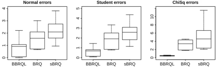
It is clear that this results in a very large number of performance measures, i.e. three different performance measures for eight parameters to estimate and this for nine data generating processes using four different modeling tech-niques. As a consequence it is not feasible to give all individual results, but instead we choose to group the results by modeling technique, performance measure and error distribution. This still gives us nine different box-plots to analyze. 0.0 0.5 1.0 1.5 2.0 2.5 Normal errors BBRQL BRQ sBRQ 0.0 0.5 1.0 1.5 2.0 2.5 Student errors BBRQL BRQ sBRQ −2 0 1 2 3 4 ChiSq errors BBRQL BRQ sBRQ
Fig. 1 Model performance in terms of bias.
Figure 1 gives us an overview of the performance of the models in terms of bias. Bias gives the expected difference between the true parameter values and the point estimates (or Bayes estimates). Larger bias indicates that the point prediction (or Bayes estimate) is further away from the true parameter value. Thus, lower bias means better performance. The plots clearly show that the proposed approach outperforms the frequentist approaches. For all error distributions considered, the bias is considerably lower for both Bayesian method.
Figure 2 plots the root mean squared error (RMSE) for every method and every error distribution that was considered. RMSE is a measure that represents how stable or how consistent the estimator is. Larger values indicate that the estimated point predictions (or Bayes estimates) fluctuate largely around the true parameter value. Lower values are thus preferred.
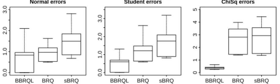
0 1 2 3 4 Normal errors BBRQL BRQ sBRQ 0 1 2 3 4 5 Student errors BBRQL BRQ sBRQ 0 2 4 6 8 10 ChiSq errors BBRQL BRQ sBRQ
Again, the results show that the proposed approach outperforms the ex-isting frequentist approaches. The RMSE is considerably lower for the lasso procedure. Similar as the results in terms of bias, the lasso outperforms the other methods for normal, Chi-square and Student errors.
Figure 3 plots the mean absolute error (MAE). Similar as RMSE, the MAE is a measure that indicates how stable or how consistent the estimator is. Again, larger values indicate that the the estimated point predictions (or Bayes estimates) fluctuate largely around the true parameter value. Contrary to RMSE, the MAE is not influenced by outliers. In this context this means that if a small minority of the 1000 Monte Carlo replications were extremely bad, this would not influence the MAE as much as it would influence RMSE.
0.0 1.0 2.0 3.0 Normal errors BBRQL BRQ sBRQ 0.0 1.0 2.0 3.0 Student errors BBRQL BRQ sBRQ 0 1 2 3 4 5 ChiSq errors BBRQL BRQ sBRQ
Fig. 3 Model performance in terms of MAE.
The boxplots of the MAE show that the proposed approach have better results compared to the frequentist methods. As with the previous perfor-mance measures, the Lasso outperforms the other methods in the case of the asymmetric Chi-square errors.
4.2 Pima Indian example
The well-known Pima Indian dataset available in the UCI machine learning repository, was analyzed using the proposed Bayesian hierarchical models. The data set consists 8 variables and 532 cases. The dependent variable is whether adult females of Pima Indians will test postitive or negative for diabetes us-ing seven covariate measurements. These measurments include the number of pregnancies (npreg), plasa glucose concentration in an oral glucose tolerance test (glu), diastolic blood pressure (dp), triceps skin fold thickness (skin), body mass index (bmi), diabetes pedigree function (ped), and age in years (age).
We treat the hyperparameters of inverse gamma prior as unknowns and estimate them along with other parameters. Three different quantiles were es-timated, that is the first quartile, the median and the third quartile. For each analysis, we ran the algorithm for 20,000 iterations. The number of burn-in iteration discarted was chosen based on the trace plots of the MCMC estima-tion and varied per quantile. To shrinkage the insignificant coefficient to zero
we used a threshold value, c = 0.1, such that the standardized effect βj is included if βjσj/σs >0.1 (Hoti and Sillan¨a¨a, 2001), where σj is the sample variance of covariatej andσp is the true variance.
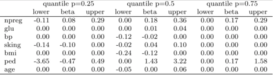
Table 1 Results of binary quantile regression with lasso on Pima dataset. quantile p=0.25 quantile p=0.5 quantile p=0.75 lower beta upper lower beta upper lower beta upper npreg -0.11 0.08 0.29 0.00 0.18 0.36 0.00 0.17 0.29 glu 0.00 0.00 0.00 0.00 0.01 0.04 0.00 0.00 0.00 bp 0.00 0.00 0.00 -0.12 -0.02 0.00 0.00 0.00 0.00 sking -0.14 -0.10 0.00 -0.02 0.04 0.10 0.00 0.00 0.00 bmi 0.00 0.00 0.00 -0.24 -0.12 0.00 0.00 0.00 0.00 ped -3.65 -0.47 0.49 0.00 1.43 3.22 0.00 0.17 1.58 age 0.00 0.00 0.00 -0.05 0.00 0.06 0.00 0.00 0.00
Table 1 shows the results of the binary quantile regression with lasso for different quantiles (i.e.p=0.25,p=0.50 andp=0.75) for the method proposed in this study. For comparison purposes, we also included the results of logis-tic regression in Table 2. The tables contain the 95% credible or confidence intervals and the posterior means and maximum likelihood estimates for the Bayesian and frequentist methods respectively.
Table 2 Result of logit model on Pima dataset. logit
lower beta upper npreg 0.00 0.12 0.24 glu 0.10 0.02 0.03 bp -0.09 -0.06 -0.33 sking 0.00 0.04 0.08 bmi -0.13 -0.06 0.01 ped 0.05 1.16 2.31 age -0.01 0.03 0.07
The results show that both the quantile model for p=0.5 and the logistic regression model give very similar results. Furthermore, the results from the quantile regression model show that not all variables exert an effect over the entire response distribution. For example the variable skin has a negative influence on the first quartile of the response distribution, while it has no effect on the other quantiles that were estimated. The opposite is true for the variable ped. This variable show to be important in the middle and high quantiles, but is irrelevant for the lower quartile. These effects would have been totally missed when analysed with popular approaches such as logit or probit models.
5 Conclusion
In this paper, we have presented a Bayesian approach for binary quantile re-gression combined with a variable selection technique, i.e. Bayesian binary quantile regression with lasso penalty. The main advantages of this approach are: first, the estimation and variable selection procedure is insensitive with regard to outliers, heteroskedasticity or other anomalies that can break exist-ing methods down. And second, the method can identify which variables are important predictors for the different quantile of the response distribution of the dependent variable.
In this paper, an l1 regularization method is proposed for binary quantile regression so that the individual effects are shrunken towards a common value. A Bayesian approach to this problem is to put Laplace prior distributions on the regression parameters. A conceptional result is that by doing so, the binary regression model is moved from a Gaussian to a full Laplacian framework and this without sacrificing much computational efficiency because of an efficient Gibbs sampling algorithm that was developed.
The applicability of the methodologies proposed was shown on both simu-lated as well as real-life data. The results showed that the Monte Carlo exper-iments strongly favoritized the new approach compared to the existing ones. That is, for every performance measure or every type of data generating pro-cess the lasso showed best performance.
Finally, the method proposed was also applied to a real-life dataset. In this kind of setting, researchers often rely to logit or probit models that are known to be biased by outliers, heteroskedasticity etc. The current method does not have this shortcoming and thus could be valuable approaches in this research setting. However, we are convinced that also in many other fields researchers could benefit from the attractive properties of the Bayesian lasso combined with binary quantile regression.
References
Alhamzawi R, Yu K (2011) Power Prior Elicitation in Bayesian Quantile Re-gression. Journal of Probability and Statistics doi:10.1155/2011/874907. Alhamzawi R, Yu K (2012) Conjugate Priors and Variable
Se-lection for Bayesian Quantile Regression. Comp Stat Data An doi:10.1016/j.csda.2012.01.014.
Alhamzawi R, Yu K, Benoit DF (2012) Bayesian Adaptive Lasso Quantile Regression. Stat Model 12:279-297.
Andrews DF, Mallows CL (1974) Scale Mixtures of Normal Distributions. J Roy Stat Soc B Met 36:99–102.
Barndorff-Nielsen OE, Shephard N (2001) Non-Gaussian Ornstein-Uhlenbeck-Based Models and Some of Their Uses in Financial Economics. J Roy Stat Soc B Met 63:167–241.
Benoit DF, Van den Poel D (2012) Binary Quantile Regression: A Bayesian Approach Based on the Asymmetric Laplace Distribution. J App Econom 27:1174–1188.
Dunson DB, Taylor JA (2005) Approximate Bayesian Inference for Quantiles. Nonparametric Statistics 17:385–400.
Florios K, Skouras S (2008) Exact Computation of Max Weighted Score Esti-mators. J Econometrics 146:86–91.
Geweke J (1991) Efficient Simulation from the Multivariate Normal and Student-t Distributions Subject To Linear Constraints. Proceedings of the 23d Symposium on the Interface 571–578.
Hoti F, Sillanp¨a¨a MJ (2006) Bayesian Mapping of Genotype 3 Expression Interactions in Quantitative and Qualitative Traits. Heredity 97:4–18. Koenker R (2004) Quantile Regression for Longitudinal Data. J Multivariate
Anal 91:74–89.
Koenker R (2005) Quantile Regression. Cambridge University Press, New York.
Koenker R, Bassett G (1978) Regression Quantiles. Econometrica 46:33–50. Koenker RW, D’Orey V (1987) Algorithm AS 229: Computing Regression
Quantiles. Appl Statist 36:383–393.
Koenker R, Machado J (1999) Goodness of Fit and Related Inference Processes for Quantile Regression. J Am Stat Assoc 94:1296–1310.
Kordas G (2006) Smoothed Binary Regression Quantiles. J Appl Econom 21:387–407.
Kozumi H, Kobayashi G (2011) Gibbs Sampling Methods for Bayesian Quan-tile Regression. J Stat Comput Sim 81:1565–1578.
Lancaster T, Jun SJ (2010) Bayesian Quantile Regression Methods J App Econom 25:287–307.
Li Q, Xi R, Lin N (2010) Bayesian Regularized Quantile Regression. Bayesian Analysis 5:1–24.
Li Y, Zhu J (2008) L1-Norm Quantile Regression. J Comput Graph Stat 17:163–185.
Manski CF (1975) Maximum Score Estimation of the Stochastic Utility Model of Choice. J Econometrics 3:205–228.
Manski CF (1985) Semiparametric Analysis of Discrete Response: Asymptotic Properties of the Maximum Score Estimator. J Econometrics 27:313–333. Michael JR, Schucany WR, Haas RW (1976) Generating Random Variates
Us-ing Transformations with Multiple Roots. The American Statistician 30:88– 90.
Park T, Casella G (2008) The Bayesian Lasso. J Am Stat Assoc 103:681–686. R Development Core Team (2011) R: A Language and Environment for
Sta-tistical Computing. URL: http://www.R-project.org
Sun W, Ibrahim JG, Zou Fei (2010) Genomewide Multiple-Loci Mapping in Experimental Crosses by Iterative Adaptive Penalized Regression. Genetics 185:349–359.
Tibshirani R (1996) Regression Shrinkage and Selection Via the Lasso. J Roy Stat Soc B Met 58:267–288.
Tsionas EG (2003) Bayesian Quantile Inference J Stat Comput Sim 73:659– 674.
Wang H, Li G, Jiang G (2007) Robust Regression Shrinkage and Consistent Variable Selection Through the LAD-Lasso. J Bus Econ Stat 25:347–355. Wu Y, Liu Y (2009) Variable Selection in Quantile Regression. Stat Sinica
19:801–817.
Yi N, Xu S (2008) Bayesian LASSO for Quantitative Trait Loci Mapping. Genetics 179:1045–1055.
Yu K, Lu Z, Stander J (2003) Quantile Regression: Applications and Current Research Area. Statistician 52:331–350.
Yu K, Moyeed RA (2001) Bayesian Quantile Regression. Stat Probabil Lett 54:437– 447.
Yu K, Stander J (2007) Bayesian Analysis of a Tobit Quantile Regression Model. J Econometrics 137:260–276.
Zheng S (2012) QBoost: Predicting Quantiles with Boosting for Regression and Binary Classification. Expert Syst Appl 39:1687–1697.
Zou H (2006) The Adaptive Lasso and Its Oracle Properties. J Am Stat Assoc 101:1418–1429.