John Carroll University
Carroll Collected
2018 Faculty Bibliography
Faculty Bibliographies Community Homepage
Spring 2018
The Propensity to Split and CEO Compensation
Erik DeVos
University of Texas at El Paso
William B. Elliott
John Carroll University, [email protected]
Richard S. Warr
North Carolina State University at Raleigh
Follow this and additional works at:
https://collected.jcu.edu/fac_bib_2018
Part of the
Finance and Financial Management Commons
This Article is brought to you for free and open access by the Faculty Bibliographies Community Homepage at Carroll Collected. It has been accepted
for inclusion in 2018 Faculty Bibliography by an authorized administrator of Carroll Collected. For more information, please [email protected].
Recommended Citation
DeVos, Erik; Elliott, William B.; and Warr, Richard S., "The Propensity to Split and CEO Compensation" (2018).2018 Faculty Bibliography. 13.
The Propensity to Split and CEO
Compensation
Erik Devos, William B. Elliott, and Richard S. Warr
∗We analyze the relation between the delta and vega of a chief executive officer’s (CEO) com-pensation and the propensity of the firm to engage in a split. Controlling for other well-known factors, we find that CEOs with compensation that has higher levels of delta are more likely to split their shares. Furthermore, the choice of split factor is inversely related to delta. Our results are economically significant: for the average (median) firm in our sample, a stock split results in
a CEO wealth gain of$4.9 million ($84,000).
Early studies of stock splits document a strong and positive abnormal return upon their an-nouncement (see, e.g., Ikenberry, Rankine, and Stice, 1996). Subsequent authors have attempted to identify factors that either trigger stock splits or that are related to the abnormal announcement returns resulting from the split announcement. Researchers have posited a variety of explanations for stock splits, including signaling to reduce information asymmetry (Brennan and Copeland, 1988; Dharan and Ikenberry, 1995; Ikenberry et al., 1996), adjusting the stock price to an optimal trading range (Copeland, 1979; Fernando, Krishnamurthy, and Spindt, 2004; Dyl and Elliott, 2006) or to an optimal tick size (Angel, 1997; Harris, 1997), and to increase the tax option value for investors (Lamoureux and Poon, 1987). In addition to the announcement return effect, beginning with Ohlson and Penman (1985), research has documented a significant increase in post-split stock volatility.
In this article, we examine whether the composition of a chief executive officer’s (CEO)
compensation portfolio increases the likelihood that the firm will announce a stock split.1Because
the announcement of a stock split frequently results in a substantial increase in both the price level and the return volatility, we hypothesize that a CEO whose compensation portfolio is sensitive to
these effects would be more likely to favor a stock split.2We base our theses on the broad idea
that CEOs with option and stock compensation portfolios benefit from stock splits in two broad ways. First, an increase in the stock price associated with the split announcement will increase the We thank Edward A. Dyl, Vincent Intintoli, Murali Jagannathan, Srini Krishnamurthy, Raghu Rau (Editor), Ousmane Seck, an anonymous referee, seminar participants at North Carolina State University and University of Texas–El Paso, and session participants at the 2010 meetings of the Financial Management Association for helpful comments. The authors gratefully acknowledge the contribution of Thomson Financial for providing analyst data available through Institutional Brokers’ Estimate System (IBES). These data were provided as part of a broad academic program to encourage earnings expectations research. We retain responsibility for any remaining errors.
∗Erik Devos is a Professor of Finance and holds the J.P. Morgan Chase Professorship in Business Administration in the
CollegeofBusinessAdministrationattheUniversityofTexas–ElPasoinElPaso,TX.WilliamB.ElliottisaProfessorof FinanceandholdstheEdwardJ.andLouiseE.MellenChairinFinanceintheBolerSchoolofBusinessatJohnCarroll UniversityinUniversityHeights,OH.RichardS.WarrisProfessorofFinanceinthePooleCollegeofManagementat NorthCarolinaStateUniversityinRaleigh,NC.
1Inanunpublishedworkingpaper,Baghai-WadjiandGabarro(2009)suggestalinkbetweenCEOstockownershipand
stock splits.
2Obviously,aCEOmaynotunilaterallycausethefirmtosplititsshares.Ataminimumthisdecisionrequiresavoteof
value of both the equity portion of their portfolio and the value of the options in their portfolio. Second, the increase in price volatility associated with a split will increase the value of the options in the CEO’s portfolio.
Evidence that CEOs know of the economic effects of splits comes from a variety of sources. First, survey evidence suggests that CEOs are aware of the positive stock price effects of an-nouncing a split. For example, in Baker and Powell’s (1993) survey of the management of 251 firms, 73.3% of the respondents agreed with the statement: “A stock split has a favorable market reaction on a firm’s stock price.” Second, evidence exists that suggests managers time splits to benefit the firm (e.g., Dyl and Elliott, 2006; Baker, Greenwood, and Wurgler, 2009). Third, anecdotal evidence suggests that managers are keenly aware of the positive stock price effects surrounding the split announcement. For example, in 2012, Tim Cook, in response to a question
from a stockholder stated that a stock split results in a “short-term pop.”3 Apple announced a
7-for-1 (7:1) split on April 23, 2014, which was greeted by an 8% stock price increase.4 Also,
Starbucks’ CEO, Howard Schultz, believes that shareholders get more excited about a stock
split announcement than any other firm announcement.5Finally, Devos, Elliott, and Warr (2015)
provide evidence that CEOs are cognizant of the effects that stock split announcements may have on their compensation portfolios. They report significant clustering of new option grants
before splits and increased levels of stock sales immediately after splits.6 They conclude that
these actions are unlikely to be random and are consistent with the conjecture that option grants to CEOs are timed such that the CEOs benefit from the largely value-increasing effect of a stock split.
To quantify how the price and volatility effects of a split might affect a CEO, we use the metrics developed by Guay (1999) and Core and Guay (2002), delta (the sensitivity of CEO wealth to a 1% change in stock price, stated in thousands of dollars) and vega (the sensitivity of CEO wealth
to a 1% change in the standard deviation (SD) of stock returns, stated in thousands of dollars),
to study the effect of the CEO’s compensation portfolio on the decision to split. As noted by Coles, Daniel, and Naveen (2006) and Core and Guay (2002), delta and vega are superior to other proxies (e.g., number of options held, value of options held, and number of options granted) of the sensitivity of CEO compensation to changes in the value and volatility of the firm’s stock.
Our article makes several contributions to the literature. First, after controlling for known determinants of splits, we show that the decision to split is directly related to the delta of the CEO’s compensation portfolio. This result is not only statistically significant, but we contend that it is also economically significant. The average (median) CEO wealth gain (in terms of her stock and option portfolio) is about $4.9 million ($84,000). To our knowledge, we are the first to examine the relation between CEO compensation and the propensity to announce a stock split. A potential criticism of our study is that stock splits tend to occur after significant price run ups and the financial benefit to the CEO of doing a stock split is probably relatively small compared to the recent wealth gains that she has experienced because of the stock price run up. We cannot refute this claim, but we can compare the economic significance of our results with those of other papers that examine CEO actions relative to their personal gain. For example, Aboody and Kasznik (2000,) in their study of information disclosures around stock grants find that CEOs have a median gain of about $18,500. They argue that this amount is an economically
3http://fortune.com/2012/02/23/no-apple-dividend-today/.
4http://www.businessinsider.com/why-tim-cook-decided-to-do-a-7-for-1-stock-split-2014-4.
5http://www.bizjournals.com/seattle/blog/2015/03/starbucks-announces-2-for-1-stock-split-investors.html.
6Specifically, Devos et al. (2015) find that timing grants before a split results in an average gain per CEO of about
meaningful incentive for CEOs and when compared to our economic estimates, this suggests that our documented wealth effect is economically meaningful as well.
Second, the prior literature posits that the motivations for splitting differ by the split factor (e.g., Desai, Nimalendran, and Venkataraman, 1998; Kamara and Koski, 2001). We find that the delta of the CEO’s compensation portfolio is negatively related to the split factor. Empirically, we also find that the announcement price reaction is unrelated to the split factor. These two results, when combined, suggest that high-delta CEOs may prefer smaller split sizes because these allow a firm to split more frequently and provide larger wealth gains in the long run.
When we bifurcate our sample by the split factor, we find that large split factors (2:1 or greater) exhibit larger post-split increases in volatility. In our tests, we find that vega is positively related to split size, although economically the importance of delta dominates the vega effect. Therefore, we doubt that vega is driving split factor sizes.
Third, we find evidence that is consistent with the premise that executive compensation (i.e., the delta of the CEO’s compensation portfolio) helps align managerial activities (in this case, engaging in a stock split that raises the share price and increases the volatility of the returns)
with those of stockholders.7We find that the likelihood of undertaking a stock split is positively
related to delta but not to the vega of the CEO’s stock and option compensation portfolio. This finding lends some support to the view that options reward value-enhancing activities.
Our final contribution is to provide further evidence, using a more recent sample, on the characteristics of splitting firms as well as some of the effects of splitting. For example, we provide evidence that abnormal returns around the announcement date remain positive and significant, though at a level of approximately 2% rather than the 3% return found using earlier
sample periods.8 We also document that the Ohlson and Penman (1985) finding, of increased
post-split price volatility, persists even after the decimalization of market prices.
The rest of the article proceeds as follows: Section I provides a brief literature review and Section II describes the hypotheses. Section III contains a description of the data and methods employed, and a univariate analysis of the splitting and nonsplitting firms. Section IV presents our multivariate results. Section V reports the analysis related to the split factor and contains additional tests. Section VI discusses the economic significance of our findings and Section VII states our conclusions.
I. Literature Review
Our article is related to two distinct areas of the literature. First, we review the literature on the causes and effects of stock splits. Second, we discuss findings on executive compensation, specifically the role of option-based compensation and executive risk-taking incentives.
A. The Effects and Determinants of Stock Splits
When a firm announces and implements a stock split, there is typically a positive price reaction on both the announcement day and the ex-date. For example, Ikenberry et al. (1996) report a mean
abnormal return of 3.38% for 2:1 stock splits (N=1,275) initiated by New York Stock Exchange
7Several researchers have attempted to use regulatory shocks to investigate the relation between risk taking and incentive
compensation. Hayes et al. (2012) use changes in stock option expensing regulations and Low (2009) uses changes in takeover protection in Delaware during the mid-1990s.
8However, our sample firms tend to be relatively large (S&P 1500 firms) and our method may differ in that we report
(NYSE) and American Stock Exchange (AMEX) firms from 1975 to 1990. However, they report a declining trend in announcement returns. In a more recent study covering 1975-2004, Lin, Singh, and Yu (2009) report an announcement return of more than 3%. Nayar and Rozeff (2001) provide evidence that the market reacts positively on the ex-date.
In addition to the positive price reaction, there is also an increase in daily return volatility. Ohlson and Penman (1985) calculate volatility as the mean of the squared daily returns for the 252 days before and after the split ex-date and find an increase in daily return volatility of about 30% beginning on the split ex-date. Their results hold for both daily and weekly data and are not temporary, but they are unable to identify any rational explanation for the effect. Subsequent work on this effect by Sheikh (1989) suggests that this volatility increase is reflected in the implied volatility of options on splitting firms. Koski (1998) finds the volatility increase remains, even after controlling for bid-ask measurement error and price levels.
Although there are numerous explanations for splits, Easley, O’Hara, and Saar (2001) categorize them into three broad subgroups: the trading range hypothesis, the reduction of information asymmetries hypothesis, and the optimal tick size hypothesis.
The trading range hypothesis, first posited by Copeland (1979), suggests that managers desire to have their firm’s shares traded at a particular stock price to attract specific clienteles. Lakonishok and Lev (1987) find that firms are likely to split their stock to maintain prices in line with a marketwide and industrywide average price, as well as a firm-specific price. Evidence consistent with the clientele effect is provided by Dyl and Elliott (2006), Fernando et al. (2004), Gompers and Metrick (2001), and Maloney and Mulherin (1992). More recently, Baker et al. (2009) suggest that managers seek a particular share price to mimic firms with high valuations.
Several papers have hypothesized that splitting behavior may be an attempt to reduce informa-tion asymmetry by revealing private informainforma-tion or attracting atteninforma-tion to the firm. Brennan and Copeland (1988) suggest that splits are a signal of improved performance; however, Lakonishok and Lev (1987) and Asquith, Healy, and Palepu (1989) provide evidence of performance increases before the split, not after. Dharan and Ikenberry (1995) and Ikenberry et al. (1996) find positive abnormal performance after the split. Brennan and Copeland (1988) find that the number of shares outstanding is related to the announcement return, and Brennan and Hughes (1991) find that changes in analyst coverage are related to the split factor. Others conclude the opposite; for example, Desai et al. (1998) use a spread decomposition approach and conclude that information asymmetry does not decrease after a split.
Angel (1997) and Harris (1997) suggest that splitting behavior is related to tick size. Firms split to increase the ratio of minimum tick size and share price such that dealers are induced to provide increased liquidity for the stock (see Schultz, 2000; Kadapakkam, Krishnamurthy, and Tse, 2005).
Others have examined the effects of split factors. For example, McNichols and Dravid (1990) suggest the split factor is related to the amount of private information disclosed.
B. Executive Compensation Incentives
To diminish the agency problems related to managerial risk aversion and better align managerial risk-taking behavior with their own, shareholders often use equity-based compensation (Jensen and Meckling, 1976). Equity-based compensation also mitigates perquisite consumption and increases effort levels. Stock options in particular have become an increasingly popular element of equity-based compensation. According to Hall and Murphy (2003), from 1992 to 2000, there was a 10-fold increase in the value of options granted to top managers of S&P 500 firms. However, following the recession of 2001, by 2004 the total value of options granted had fallen by more
than 50% of the 2002 level. Overall, this decline in option grants was temporary, as Cao and Wang (2013) note that from 1994 to 2009, median incentive pay increased by 244% in real terms whereas firm value increased only 40% during the same period.
The importance of equity-based compensation has resulted in a substantial literature being developed that analyzes the relation between CEO equity-based compensation, risk taking, and
firm performance.9 During the last decade or so, primarily based on insights provided by Core
and Guay (2002), researchers have begun to use delta (the sensitivity of compensation to a change in the stock price) and vega (the sensitivity of compensation to a change in the stock volatility) as measures of managerial compensation and incentives. Empirically, the evidence linking delta and vega to corporate policies is mixed. Cohen, Hall, and Viceira (2000) find that increases in option compensation leads to increases in firm risk; however, they fail to find a significant stock return response to option-induced risk taking and conclude that the effect is relatively small. Coles et al. (2006) find that higher levels of vega are associated with a greater propensity to take risk-increasing actions, including more research and development (R&D) spending, less spending on fixed assets, greater firm focus, and higher proportions of debt. However, Hayes, Lemmon,
and Qiu (2012) find that vega does not seem to be related to risk-taking activities.10
II. Hypotheses Development
A major finding of the compensation literature, as discussed above, is that delta and vega are effective proxies for measuring the degree to which CEO incentives are aligned with those of shareholders. Combined with the empirical fact that a large fraction of stock splits lead to announcement and ex-date price appreciation as well as increased price volatility in the year following the split, we hypothesize the following:
H1a: CEOs with stock and option compensation that is more sensitive to share price increases (i.e., high delta component) are more likely to split their firm’s shares.
H1b: CEOs with stock and option compensation that is more sensitive to volatility (i.e., high vega component) are more likely to split their firm’s shares.
Our second hypothesis examines the relation between the split factor and the delta of the CEO’s compensation portfolio. If a CEO’s wealth increases when she conducts a stock split, then rationally, a CEO would prefer to conduct more, rather than fewer, splits. Empirically, we find no statistical relation between the average announcement return and the split factor. Therefore, given this lack of correlation between the announcement return and the split factor, a CEO whose compensation portfolio has a relatively high delta (ceteris paribus) would likely select a smaller split factor. This is because a smaller factor will result in approximately the same average announcement and ex-date price increase as compared to a larger split factor. Therefore, for a given share price increase over a given period, the CEO could engage in more splits with smaller factors. Specifically, we hypothesize the following:
9See Core, Guay, and Larcker (2003) for a survey of this literature.
10Compensation-induced risk-taking behavior may result in negative consequences for shareholders. For example, Cheng
and Warfield (2005) find that equity incentives (i.e., delta) are related to earnings management. Johnson, Ryan, and Tian (2009) find that delta is related to accounting fraud; Efendi, Srivastava, and Swanson (2007) and Burns and Kedia (2006) find that delta is related to accounting misstatements. Bergstresser and Philippon (2006) find that delta is related to accruals. Conversely, Erickson, Hanlon, and Maydew (2006) and Armstrong, Jagolinzer, and Larcker (2010) find that stock-based compensation (delta) is not related to accounting fraud accusations and other accounting irregularities.
H2: CEOs with stock and option compensation that is more sensitive to share price increases (i.e., high delta component) are more likely to select a smaller split factor.
It is also possible that vega is correlated with the split factor. For example, if larger split factors are associated with greater post-split price volatility, CEOs whose compensation portfolios have high levels of vega may prefer a larger split factor. However, we think that this is unlikely to occur, for two reasons. First, the delta effects appear to dominate the vega effects by an order of magnitude. Second, although a price increase can have a direct realizable impact on CEO wealth, a volatility increase is harder to capitalize on given the nontradability of executive stock options.
III. Data and Methods
A. Sample
We use the ExecuComp database to compute a delta and vega for each firm with available data
between 1992 and 2005.11This produces a sample of 21,414 firm-years covering 2,704 unique
firms. We then gather the financial accounting data necessary to compute our control variables from Compustat. Because of missing data or nonpositive assets or revenues, the sample size decreases to 20,863 firm-years and 2,643 unique firms. Market data and split data are gathered from the Center for Research in Security Prices (CRSP) database. Any firm in the sample that has a CRSP distribution code of 5523 and a CRSP share factor of at least 0.5 (i.e., engages in at least a 3:2 split) at any time during the sample period is identified as a stock split. We find 1,837 splits made by 1,107 unique firms. We also gather return data around the split declaration and ex-dates as well as price data (to compute price appreciation in the preceding years as well as price volatility in the post-split year) from CRSP.
We filter the sample to remove extreme outliers and potential coding errors with the following restrictions. The share price must be greater than $5 and less than $10,000. We remove firms
with a debt-to-assets (Compustat item #181÷#6) or debt-to-equity (#181÷[#6−#181]) ratio
greater than 1 or 500, respectively. We restrict the sample to firms that have a positive value for total common equity (#60). Finally, to allow computation of a price appreciation measure, we
require that the firm exist in the CRSP database for three years before the sample year.12 The
final sample has 19,178 firm-years from 2,501 unique firms. During the sample period, there were a total of 1,617 splits made by 1,027 firms.
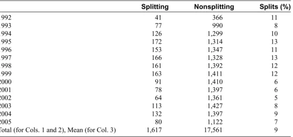
We show the temporal distribution of splitting and nonsplitting firms in Table I. The table provides several insights. First, there are 1,617 stock splits and 17,561 firm-years in which firms do not split. Second, the number of splits during a given year ranges from 41 (in 1992) to 172 (in 1995). As a percentage of all sample firms, on an annual basis, between 5% (in 2002) and 13% (in 1995 and 1997) of firms split. For most years this percentage is around 10%. Only 2000–2002 seems to have a smaller number of splits.
11The database contains, among other variables, complete details related to executive stock and option grants for more
than 3,300 firms. From the ExecuComp data description manual: “The universe of firms cover the S&P 1500 plus companies that were once part of the 1500 plus companies removed from the index that are still trading, and some client requests. Data collection on the S&P 1500 began in 1994. However, there is data back to 1992 but it is not the entire S&P 1500.” Several key variables were reported during this period that enable us to compute the vega and delta. After 2005, these key variables were no longer recorded.
Table I. Stock Splits by Year
This table presents the number of splitting (firms that engage in at least a 3:2 stock split) and nonsplitting firms by year.
Splitting Nonsplitting Splits (%)
1992 41 366 11 1993 77 990 8 1994 126 1,299 10 1995 172 1,314 13 1996 153 1,347 11 1997 166 1,328 13 1998 161 1,392 12 1999 163 1,411 12 2000 91 1,410 6 2001 78 1,397 6 2002 64 1,361 5 2003 113 1,427 8 2004 132 1,397 9 2005 80 1,122 7
Total (for Cols. 1 and 2), Mean (for Col. 3) 1,617 17,561 9
B. Price and Volatility Effects around Splits
Our hypotheses critically depend on whether splits lead to positive returns around the an-nouncement date and increased volatility after the split. In Table II, we show abnormal returns around the announcement dates and ex-dates, and pre- and post-split volatility. We calculate
two-day (two-day 0 to+1) and three-day (day−1 to+1) market-adjusted holding period returns on the
announcement and ex-dates of the split using the CRSP value-weighted dividend-adjusted returns as the market index. Our results are generally consistent with the previous literature. The mean (median) three-day market-adjusted announcement return is about 2.0% (1.3%). This return is
lower than Ikenberry et al. (1996), who report a mean of 3.38% for 2:1 stock splits (N=1,275)
initiated by NYSE and AMEX firms from 1975 to 1990.13However, they report a declining trend
in announcement returns.14The mean market-adjusted return around the ex-date is approximately
0.6%. We also report a compound return for the announcement plus ex-date (using a three-day window around each date). The mean (median) compound return is 2.5% (1.9%). To determine whether volatility increases after the split, we follow Ohlson and Penman (1985), who calculate volatility as the mean of the squared daily returns for the 252 days before and after the split ex-date. The mean (median) volatility before the split is 0.0008 (0.0004), whereas after the split the mean (median) increases to 0.0011 (0.0006). In other words, the average daily volatility increases by about 37%. Ohlson and Penman (1985) report a nearly 30% increase in daily volatility during
their earlier sample period. This is approximately equivalent to an annual mean (median)SDof
returns of 44.9% (31.7%) before the split and 52.6% (38.9%) after the split.
A pairwise test for the difference in pre- and postyear volatility shows that this increase is statistically significant (the mean difference is 0.0003). In addition, more than 70% of the
13The Ikenberry et al. (1996) return spans five days, from day−2 to day+2 around the split announcement.
Table II. Price Effects of Stock Splits
This table presents market-adjusted returns over various windows as well as pre- and post-split return volatility. Panel A displays the average compounded announcement date and ex-date returns for stock splits with a split factor of at least 1.5 (i.e., 3:2) between 1992 and 2005. We use the CRSP value-weighted dividend-adjusted returns for the market. In Panel B, volatility is calculated as the mean squared daily return for the 252 trading days on either side of the ex-date. In the third row of the panel, paired difference in
volatility is calculated using a (pairwise)t-test.
Split Sample (N=1,617) Mean Median Panel A. Returns Announcement date (0 to+1) 0.0175∗∗∗ 0.0121∗∗∗ Announcement date (−1 to+1) 0.0196∗∗∗ 0.0132∗∗∗ Ex-date (0 to+1) 0.0037∗∗∗ 0.0013∗∗∗ Ex-date (−1 to+1) 0.0058∗∗∗ 0.0028∗∗∗
Compound announcement (−1 to+1) and ex-date (−1 to+1) 0.0254∗∗∗ 0.0186∗∗∗
Panel B. Volatility
Pre-split 0.0008∗∗∗ 0.0004∗∗∗
Post-split 0.0011∗∗∗ 0.0006∗∗∗
Paired difference (post – pre) 0.0003∗∗∗ 0.0002∗∗∗
∗∗∗Significant at the 0.01 level.
splitting firms show increased volatility. This finding is consistent with Ohlson and Penman (1985) and may provide the impetus for CEOs to split their shares, especially when the vega component of the CEO’s compensation package is relatively high.
C. Hypothesis Testing
To test our hypotheses, we examine the extent to which delta and vega are associated with the decision to split using a logistic regression model with additional control variables (see Equation (1)).
P(Spli tj,t =1|xj,t)=G(xj,t, α), (1)
where G(xj,tα)= 1
1+e−x j,tα andxj,t α = α0 +α1 {CEO Compensation Measures}j,t−1 + α2
{Trading Range Controls}j,t−1+α3{Information Asymmetry Controls}j,t−1+α4{Optimal Tick
Size Controls}j,t−1+α5market-to-bookj,t−1+α6ln[totalassetsj,t−1].15
CEO compensation measures are the sensitivity of CEO compensation to changes in share
price (ln[deltaj,t−1]) and/or to changes in share price volatility (ln[vegaj,t−1]). Both variables are
calculated at the end of the previous fiscal year (denoted by subscriptt−1, whereasjrepresents
firmj). On average, a split results in an increase in both the level and the volatility of the stock
price; therefore, we expect the coefficients on ln[deltaj,t−1] and ln[vegaj,t−1] to be positive.
15To control for industry and time effects, we also include industry (based on two-digit Standard industrial classification
In addition, we include control variables commonly found in prior research. Ikenberry et al. (1996) find an inverse (direct) relation between the split abnormal announcement return and firm size (market-to-book). Although our dependent variable is the decision to split rather than the announcement return, it is likely that a similar relation may hold in our model. For this
reason, we usemarket-to-bookj,t−1, which is the market value of equity scaled by book value,
and ln[totalassetsj,t−1], which is the natural log of the book value of total assets. We follow Dyl
and Elliott (2006) and include three proxies to control for trading range explanations. The first is
traderangej,t−1, which is a binary variable that is equal to one when the actual share price is 50%
or more of the predicted share price, where predicted share price is the predicted value from an annual regression of average share price on book value of equity, average value of shareholdings,
and earnings per share (in Section III.D, we describe this variable in more detail).16The second
variable isstockapprj,t−1, which captures the amount of stock appreciation in the prior two years
(computed as the ratio of fiscal year-endsharepricet−1 tosharepricet−3, wheresharepricej,t−1
is the closing price on the last day of the fiscal year). Fortraderangej,t−1 andstockapprj,t−1, we
expect a positive relation with the likelihood of a split. The third variable isinstitownj,t−1, which is
the percentage of shares owned by institutions.17Forinstitownj,t−1, we expect a negative relation
with the likelihood of a split.
We use two variables to control for explanations based on information asymmetry: analyst
following (analystsj,t−1) and number of shareholders (shareholdersj,t−1). We expect a negative
relation for both variables with the likelihood of a split. Finally, to control for optimal tick size explanations, we use year dummies because the move from eighths to sixteenths that occurred in 1997 and the decimalization that occurred in 2001 may affect optimal tick sizes (e.g.,
Kadapakkam et al., 2005; Lipson and Mortal, 2006). These dummies are labeled
predecimaliza-tion(postdecimalization) and they equal one for firm years before (after) 1997 (2000). If firms
attempt to use a split in a Brennan and Hughes (1991) sense (i.e., increase overall gain to brokers by forcing a wider relative spread, which is expected to increase the firm’s shareholder base), we
expect a positive relation betweenpredecimalizationand the decision to split. We have no priors
with regard topostdecimalization.
D. Variable Construction and Univariate Analysis 1. Variable Measurement
We measure the sensitivity of CEO compensation to changes in equity return levels and
volatility.18 The first variable, deltat−1, is the partial derivative of the Black-Scholes (1973)
equation with respect to the stock price level, and it measures the incentive to increase the stock
price. The second variable, vegat−1, is the partial derivative of the dividend-adjusted
Black-Scholes (1973) equation with respect to theSDof stock returns, and it measures the incentive to
take risk. We computedeltaandvegafor each CEO’s stock and option portfolio to measure CEO
16In addition to these trading range controls, we also estimate the original trading range variable reported in Lakonishok
and Lev (1987), which compares the splitting firm’s stock price with that of a portfolio of comparable firms. Our results (untabulated) are robust to this test.
17Given that most trading range explanations for splitting assume that managers split in order to attract individual
shareholders (vis-`a-vis institutional shareholders), we include institutional ownership prior to the split. In additional (unreported, but available upon request) analysis we use an additional variable to capture the trading range explanation for splits, based on Lakonishok and Lev (1987). Our results do not materially change.
18We use the approach of Rogers (2002) and Core and Guay (2002) to create measures of a CEO’s incentive to engage in
risk-taking incentives.19We use Compustat data to calculate other variables used in our analyses:
market-to-bookt−1([#25×#199]÷#60),totalassetst−1(#6),netsalest−1(#12),debt-to-equityt−1
(#181÷[#6−#181]),EPSt−1(#58), andROEt−1([#25×#58]÷#60).
We now turn to the characteristics related to the three potential split explanations (trading range, asymmetric information, and tick size). First, we consider the variables that proxy for the
trading range explanation. The variabletraderanget−1indicates whether the price of the stock is
too high, and the variablestockapprt−1measures the increase in the firm’s stock price over the
two years preceding yeart.traderangej,tis defined as follows:
traderangej,t =sharepricej,t/E
sharepricej,t |BVEquityj,t,AvgHldgj,t,EPSj,t
, (2)
whereE(sharepricej,t−1|BVEquityj,t−1,AvgHldgj,t−1,EPSj,t−1) is estimated by Equation (3):
Esharepricej,t−1|BVEquityj,t−1,AvgHldgj,t−1,EPSj,t−1
=δ0+δ1BVEquityj,t−1
+δ2AvgHldgj,t−1, +δ3EPSj,t−1, (3)
whereBVEquityj,t−1 is book value of equity (#60),AvgHldgj,t−1is total equity per shareholder,
andEPSj,t−1is yeart−1 earnings per share.
We computetraderangej,t−1as the ratio of a firm’s actual share price in yeart−1 to its predicted
share price from Equation (3), conditioned on the firm’s size, average holdings per shareholder,
and earnings per share. There is no reason to expect that small differences fromtraderangej,t−1
are important, so we convert it to a binary variable that equals one if the actual share price is 50%
greater than the predicted price and zero otherwise. Thestockapprj,t−1variable is the proportional
increase in firmj’s split-adjusted average stock price during the two years preceding the split
year, and is computed as follows:
stockapprj,t−1=sharepricej,t−1/sharepricej,t−3. (4)
Institutional ownership (institownj,t−1) data from Compact Disclosure represents the ownership
by all institutions as a percentage of total shares outstanding. However, data for this variable are available only until 2004. As information asymmetry proxies, we use the number of analysts from
Institutional Brokers’ Estimate System (IBES) (analystsj,t−1) and the number of shareholders
(shareholdersj,t−1). Finally, to capture the optimal tick size explanation, we use the stock price
before the split, from CRSP. 2. Univariate Results
In Table III, we compare splitting firms with the full sample of all nonsplitting firms (which we use as the sample for the rest of the article). We also provide test statistics to assess the difference between the subsamples. Consistent with H1a and H1b, CEOs of splitting firms have
significantly higher values of delta and vega. They have a meandeltat−1(vegat−1) of 2,967 (163)
compared to 1,027 (147) for managers of nonsplitting firms. These results suggest that, as it relates to stock splits, managers whose compensation has greater incentives to increase price and risk may indeed do so.
19For pure stock holdings, delta=1 and vega=0. A detailed description of the calculation of delta and vega is provided
Table III. Sample Firm Characteristics This tab le presents the uni v ariate characteristics for splitting and nonsplitting sample fir ms from 1992 to 2005. F rom Compustat, w e compute mar ket-to-book (#25 × #199 ÷ #60), total assets (#6, in $millions), net sales (#12, in $millions), debt-to-equity (#9 ÷ #60), EPS (#58), RO E (#25 × #58 ÷ #60), shar eholder s (#100, in thousands), and shar eprice (#199). tr ader ang e is a binar y v ariab le that equals one if the actual share price is 50% g reater than the predicted price (calculated follo wing Dyl and Elliott, 2006) and zero otherwise. stoc kappr is the ratio of the t − 1 y ear-end shar eprice o v er the t − 3 y ear-end shar eprice , institutional o wnership (labeled instito wn ) is from CD Disclosure, and anal yst co v erage (labeled anal ysts ) is from IBES. ve g a and delta are calculated similar to Ro gers (2002) and are stated in thousands of dollars. W e repor t dif ferences in means ( T , from a t-test) and medians ( Z , from a signed-rank test) betw een the sample and all nonsplitting fir ms. Splitting Firms ( N = 1,617) Nonsplitting Firms (All, N = 17,561) Difference (Splitting – Nonsplitting, All) Mean Median Mean Median TZ Managerial characteristics delta t − 1 2,966.63 461.33 1,027.28 211.55 3.45 ∗∗∗ 18.78 ∗∗∗ ve g at− 1 163.28 52.76 147.43 46.83 1.78 ∗ 2.49 ∗∗ F inancial characteristics mar ket-to-book t− 1 4.99 3.42 3.35 2.21 9.98 ∗∗∗ 25.55 ∗∗∗ total assets t − 1 10,195.24 1,432.36 11,504.78 1,548.87 − 1.20 − 2.31 ∗∗ net sales t − 1 4,654.40 1,183.15 4,533.66 1,213.71 0.39 − 0.41 debt-to-equity t− 1 2.50 1.08 2.85 1.37 − 3.11 ∗∗∗ − 7.23 ∗∗∗ EPS t − 1 2.53 2.09 1.44 1.34 17.09 ∗∗∗ 22.24 ∗∗∗ RO Et− 1 (%) 16.99 16.05 8.44 12.01 6.73 ∗∗∗ 21.13 ∗∗∗ T rading range controls tr ader ang et− 1 (%) 1.42 0.00 0.29 0.00 3.83 ∗∗∗ 7.11 ∗∗∗ stoc kappr t − 1 1.37 1.24 1.22 1.11 7.87 ∗∗∗ 13.03 ∗∗∗ instito wn t − 1 (%) 60.17 61.70 58.63 60.80 2.43 ∗∗∗ 2.41 ∗∗∗ Infor mation asymmetr y controls anal ysts t − 1 9.05 6.92 8.14 6.17 4.06 ∗∗∗ 3.63 ∗∗∗ shar eholder st− 1 30.73 4.33 32.91 5.51 − 0.53 − 4.64 ∗∗∗ T ick size controls shar eprice t − 1 54.75 47.88 31.52 27.19 27.13 ∗∗∗ 37.84 ∗∗∗ ∗∗∗ Signif icant at the 0.01 le v el. ∗∗Signif icant at the 0.05 le v el. ∗Signif icant at the 0.10 le v el.
Splitting firms have an average (median)market-to-bookt−1of 4.99 (3.42), whereas nonsplitting
firms have an average (median) market-to-bookt−1 of 3.35 (2.21). Both the mean and median
are significantly different at the 1% level. This finding suggests that splitting firms are relatively more highly valued and are more typically growth stocks. Splitting firms are slightly smaller in terms of assets, but have nearly the same level of annual sales. For example, the mean (median)
totalassetst−1 for splitting firms is $10.2 billion ($1.4 billion), whereas the mean (median)
totalassetst−1 for nonsplitting firms is $11.5 billion ($1.5 billion). Splitting firms have lower
debt-to-equityt−1ratios and are more profitable in terms ofEPSt−1andROEt−1, again consistent
with their being more growth-oriented stocks.
The traderanget−1 variable is equal to one if the share price is more than 50% above the
predicted price and zero otherwise.20 Only a very small, but significantly different, fraction
between splitting and nonsplitting firms is above this 50% threshold. The mean (median) value
of traderanget−1 for splitting firms is 1.42% (0.00%), whereas the corresponding value for
nonsplitting firms is 0.29% (0.00%). The mean difference is statistically significant and indicates that a significantly higher percentage of splitting firms have share prices that are “too high,” and the split will thus bring them back in line with their expected share price. Table III shows
thatstockapprt−1is significantly higher for splitting firms. We find that splitting firms had an
average stockapprt−1 of 37%, compared to 22% for nonsplitting firms. The medians show a
similar pattern.
Splitting firms have significantly higher institutional ownership (i.e., the mean for splitting firms is 60% versus 59% for nonsplitting firms; the medians show the same pattern). Al-though these differences are statistically significant, the economic significance is small. Overall, these findings suggest that trading range explanations may indeed be related to the splitting decision.
For the information asymmetry proxies, we find that splitting firms are followed by an average
(median) of 9.1 (6.9)analystst−1, whereas nonsplitting firms are followed by an average (median)
of 8.1 (6.2)analystst−1. The number of shareholders (shareholderst−1) is slightly smaller for
splitting firms. These results seem to be mixed, given that we expect firms with greater information asymmetry to have lower levels of both analyst following and number of shareholders.
We find that the mean share price is higher for splitting firms. The mean share price is more than $54 for splitting firms and about $32 for nonsplitting firms. This evidence appears to be most consistent with the trading range hypothesis.
IV. Relation between the Decision to Split and Compensation
Incentives
A. Multivariate Analysis
To further examine our primary hypotheses, namely, firms whose CEOs have compensation portfolios with a higher delta and vega are more likely to split their firm’s stock, we estimate a logit regression as described in Equation (1). The results are presented in Table IV. The table shows the
odds ratios and the correspondingp-values in parentheses. The first column models the decision
to split as a function of CEO compensation sensitivity (ln[deltat−1] and ln[vegat−1]), the
market-to-book ratio (market-to-bookt−1), and the natural log of assets (ln[assetst−1]).21Consistent with
20Our results remain qualitatively similar when we use 10% or 25%.
Table IV. Logit Analysis of Split Decision Lo git anal ysis is used to study the relation betw een the decision to split during an y gi v en y ear and measures of CEO compensation exposure to changes in share price and v olatility , as w ell as v ariab les to control for other split explanations. The dependent v ariab le equals one for splitting fir ms and zero for nonsplitting fir ms. delta is the dollar change in CEO w ealth for a 1% change in stock price and ve g a is the dollar change in CEO w ealth for a 0.01 change in SD (both delta and ve g a are stated in thousands of dollars). mar ket-to-book is the equity mark et-to-book (#25 × #199 ÷ #60), ln[ assets ] is the natural lo g of total assets (#6, in $000,000s), pr edec ( postdec ) is a dumm y v ariab le equal to one if the split occur red before 1997 (after 2000), tr ader ang e is a binar y v ariab le equal to one if the actual share price is 50% g reater than the predicted price (calculated follo wing Dyl and Elliott, 2006) and zero otherwise, stoc kappr is the ratio of the t − 1 y ear-end shar eprice o v er the t − 3 y ear-end shar eprice , institutional o wnership (labeled instito wn ) is from CD Disclosure, anal ysts is the number of anal ysts follo wing the stock (from IBES), and shar eholder s is item #100 (000s) from Compustat. W e repor t odds ratios and p -v alues are in parentheses. Model 1 Model 2 Model 3 Model 4 Model 5 Model 6 Model 7 Model 8 ln[ delta t− 1 ]1 .4 3 ∗∗∗ 1.44 ∗∗∗ 1.43 ∗∗∗ 1.44 ∗∗∗ 1.40 ∗∗∗ 1.41 ∗∗∗ 1.39 ∗∗∗ 1.39 ∗∗∗ (0.01) (0.01) (0.01) (0.01) (0.01) (0.01) (0.01) (0.01) ln[ ve g at− 1 ] 1.01 1.01 1.01 1 .01 1.00 1 .01 0.99 1 .00 (0.72) (0.63) (0.72) (0.63) (0.81) (0.73) (0.72) (0.91) mar ket-to-book t− 1 1.00 ∗∗ 1.01 ∗∗ 1.00 ∗∗ 1.01 ∗∗ 1.00 1.00 1.00 1.00 (0.04) (0.02) (0.04) (0.02) (0.27) (0.16) (0.56) (0.33) ln[ assets t− 1 ]0 .8 8 ∗∗∗ 0.87 ∗∗∗ 0.88 ∗∗∗ 0.87 ∗∗∗ 0.90 ∗∗∗ 0.88 ∗∗∗ 0.88 ∗∗∗ 0.88 ∗∗∗ (0.01) (0.01) (0.01) (0.01) (0.01) (0.01) (0.01) (0.01) pr edec t− 1 — — 2.15 ∗∗∗ 2.25 ∗∗∗ 2.13 ∗∗∗ 2.23 ∗∗∗ 2.20 ∗∗∗ 2.34 ∗∗∗ (0.01) (0.01) (0.01) (0.01) (0.01) (0.01) postdec t− 1 — — 1.18 1.20 1.20 1.23 1.13 1.15 (0.31) (0.26) (0.26) (0.21) (0.50) (0.44) tr ader ang et− 1 ———— 2 .9 2 ∗∗∗ 3.03 ∗∗∗ 2.49 ∗∗∗ 2.50 ∗∗∗ (0.01) (0.01) (0.01) (0.01) stoc kappr t− 1 ———— 1 .6 3 ∗∗∗ 1.57 ∗∗∗ 1.64 ∗∗∗ 1.57 ∗∗∗ (0.01) (0.01) (0.01) (0.01) instito wn t− 1 —————— 1 .0 1 ∗∗∗ 1.01 ∗∗∗ (0.01) (0.01) anal ysts t− 1 —————— 1 .0 1 1 .0 1 (0.20) (0.24) shar eholder st− 1 —————— 1 .0 0 1 .0 0 (0.89) (0.96) Industr y fix ed ef fects No Y es No Y es No Y es No Y es Y ear fix ed ef fects Y es Y es Y es Y es Y es Y es Y es Y es Obser v ations 19,175 19,175 19,175 19,175 19,175 19,175 15,042 15,042 Splitting fir ms 1,617 1,617 1,617 1,617 1,617 1,617 1,299 1,299 ∗∗∗ Signif icant at the 0.01 le v el. ∗∗Signif icant at the 0.05 le v el.
the univariate results in the previous section, the odds ratio of ln[deltat−1] is greater than one
and statistically significant at the 1% level. However, the coefficient on ln[vegat−1] is
insignifi-cant. Model 2 has the same variables; however, we added industry fixed effects and the result is similar. Models 3 and 4 include additional variables to control for the optimal tick-size explana-tion. The results on the CEO compensation sensitivity variables remain qualitatively unchanged. Models 5 and 6 add variables intended to control for the trading range explanation of splits, and Models 7 and 8 add controls for the information asymmetry split explanation. In all cases,
ln[deltat−1] remains significantly greater than one whereas the coefficient on ln[vegat−1]
contin-ues to be not statistically different from one. In sum, the results support H1a, though there is no support for H1b in the multivariate models. To put these numbers into perspective, at the sample
mean for ln[deltat−1] of 5.4 (which equates to adeltat−1 of 221.4), an increase to 6.4 (deltat−1
equal to 601.8) would increase the probability of a split by approximately 39%, ceteris paribus. A 1
SDshift from the mean (SD=1.718;deltat−1of 1,234.0) would increase the probability of a split
by 67%.
To assure that our results are not due to model misspecification, we conduct the
fol-lowing robustness test. Because deltat−1 and vegat−1 are positively correlated (correlation
coefficient=0.45), we estimate all the models from Table IV with only ln[deltat−1] and again
with only ln[vegat−1]. The results (untabulated) for the models that include only ln[deltat−1] are
qualitatively similar to Table IV. In the models that include only ln[vegat−1], the coefficient on
ln[vegat−1] is statistically significant in all specifications. Also, although we attempt to control
for the skewness ofdeltat−1andvegat−1using logs, as an alternative control we create an indicator
value for each variable representing the top quintile, that is, the largest 20% of values ofdeltat−1
andvegat−1. We repeat the Table IV regressions using these new variables and find qualitatively
similar results (untabulated).
V. Relation between Split Factor Choice and Compensation
Incentives
In this section, we investigate how returns and volatility shifts, following a split announcement, differ by split factor. These results are reported in Table V. For 3:2 splits, we find mean (median)
three-day (−1 to+1) market-adjusted announcement returns of 1.79% (1.22%), whereas splits
of 2:1 or larger generate mean (median) returns of 2.04% (1.40%). However, these returns are not statistically different from one another, nor are the ex-date or compound returns (accumulated across the announcement and ex-dates). Likewise, we find only marginally significant differences in volatility (only for the median) before the split. However, 2:1 splitters exhibit a mean increase in volatility of 0.0004 after the split, compared to 0.0002 for 3:2 splitters. The means and medians are significantly different across the two split factors. It appears that the split factor does not affect market-adjusted announcement or ex-date returns; however, it does affect post-split volatility. Therefore, it follows that delta and vega could have different effects on the decision to undertake a large (2:1 or greater) or small (3:2) split. Given that the returns are not different, it could be argued that delta would have little effect on the choice of split factor. However, if returns are unaffected by split factor, a rational CEO might prefer a smaller factor that would enable
more frequent splits in the future.22
22Conversely, if a large split (2:1 or greater) has a larger impact on volatility, one might expect that CEOs with relatively
more exposure to vega in their compensation portfolio (i.e., greater incentive to take on firm-specific risk) would opt for a larger split factor. However, because the CEO’s stock options are nontradable, the impact of vega may well be limited
Table V. Price Effects of Stock Splits by Split Factor This tab le presents mark et-adjusted retur ns o v er v arious windo ws as w ell as pre-and post-split retur n v olatility for small (def ined as 3:2) and lar g e (def ined as 2:1 or lar ger) split factors. P anel A displa ys the av erage compounded announcement date and ex-date retur ns for stock splits with a split factor of at least 1.5 (i.e., 3:2) betw een 1992 and 2005. W e use the CRSP v alue-w eighted di vidend-adjusted retur ns for the mark et. In P anel B , v olatility is calculated as th e mean squared dail y retur n for the 252 trading da ys on either side of the ex-date. In the third ro w of the panel, paired dif ference in v olatility is calculated using a (pairwise) t -test. 2:1 Splits or Larger 3:2 Splits Difference (2:1 − 3:2 or Larger) Mean Median Mean Median Mean Median P anel A. Returns Announcement date (0 to + 1) 0.0183 ∗∗∗ 0.0127 ∗∗∗ 0.0157 ∗∗∗ 0.0113 ∗∗∗ 1.02 0.72 Announcement date ( − 1t o + 1) 0.0204 ∗∗∗ 0.0140 ∗∗∗ 0.0179 ∗∗∗ 0.0122 ∗∗∗ 0.88 0.50 Ex-date (0 to + 1) 0.0035 ∗∗∗ 0.0007 ∗∗ 0.0041 ∗∗∗ 0.0020 ∗∗∗ − 0.28 − 0.01 Ex-date ( − 1t o + 1) 0.0061 ∗∗∗ 0.0034 ∗∗ 0.0051 ∗∗∗ 0.0011 ∗∗∗ 0.36 0.67 Compound announcement ( − 1t o + 1) and ex-date ( − 1t o + 1) 0.0263 ∗∗∗ 0.0186 ∗∗∗ 0.0236 ∗∗∗ 0.0184 ∗∗∗ 0.64 0.56 P anel B . V olatility Pre-split 0.0008 ∗∗∗ 0.0004 ∗∗∗ 0.0007 ∗∗∗ 0.0005 ∗∗∗ 1.57 2.14 ∗∗ P ost-split 0.0011 ∗∗∗ 0.0007 ∗∗∗ 0.0009 ∗∗∗ 0.0006 ∗∗∗ 3.28 ∗∗∗ 0.75 P aired dif ference (post – pre) 0.0004 ∗∗∗ 0.0002 ∗∗∗ 0.0002 ∗∗∗ 0.0001 ∗∗∗ 3.28 ∗∗∗ 3.81 ∗∗∗ ∗∗∗ Signif icant at the 0.01 le v el. ∗∗Signif icant at the 0.05 le v el.
A. Univariate Analysis
In Table VI, we present univariate results when the splitting sample is bifurcated by large versus small (i.e., 2:1 and greater vs. 3:2) split factors. The table shows that there are significant
differences between these groups. Both the mean and median for deltat−1 and vegat−1 are
significantly larger for 2:1 splitters. However, the significance levels are substantially lower
fordeltat−1.
Firms with split factors of 2:1 or greater have significantly highermarket-to-bookt−1 ratios.
They also are significantly larger when measured bynet salest−1but not when measured bytotal
assetst−1. Earnings per share (EPSt−1) for firms using large split factors are also significantly
higher.
All three variables related to the trading range explanation are different across split factors. Nearly 2% of firms using large split factors were at least 50% above their predicted price range,
whereas only 0.2% of firms using 3:2 factors were similarly situated. The level ofstockapprt−1
during the two years before the split was also slightly higher for firms using large split fac-tors. Large splitters have slightly higher institutional ownership, although the difference is of questionable economic significance (61% vs. 59%). Proxies for information asymmetry split explanations are also substantially different between the two split factors. Firms using 2:1 splits
have significantly moreanalystst−1andshareholderst−1, which suggests they exhibit relatively
less information asymmetry.
Firms that engage in larger splits have, on average, significantly higher pre-split share prices.
For example, the meansharepricet−1for large splits is $62.23, compared to a meansharepricet−1
of $37.65 for firms that split by 3:2, consistent with the optimal tick size explanation. B. Multivariate Analysis
In Table VII, we test H2 and examine the relation between the delta of CEO compensation and the split factor in a multivariate setting. Using a logistic regression, we estimate Equation (1), except in this case, the dependent variable equals one if the firm engages in a 2:1 or larger split, and zero if the split factor is 3:2. Similar to the analysis of the decision to split, we estimate eight models and include temporal fixed effects in all models and industry fixed effects in the
even-numbered models. The odds ratio for ln[deltat−1] is significant and less than one in all
eight models. A one-standard deviation increase in ln[deltat−1] (from an average of 6.17-7.84)
decreases the probability of a 2:1 (or greater) split by 15.6%. These results are the reverse of the univariate findings, in which case the CEOs of firms that engaged in larger splits (i.e., 2:1 or greater) had greater delta sensitivity (i.e., higher average levels of delta). The multivariate results suggest an inverse relation between delta and the propensity to choose a 2:1 split. At first, this may appear to be puzzling, but when viewed in light of the findings presented in Table V, this result is consistent with our hypothesis. Table V shows that statistically, there is no difference between the abnormal returns of 3:2 and 2:1 (or greater) split factors on either the announcement date or ex-date. Therefore, one could conclude that for CEOs with higher delta exposure, a smaller split factor would achieve the same increase in CEO wealth as a larger split factor, and possibly allow
for another split sooner than if a larger split factor had been chosen.23In sum, the evidence from
Table VII provides support for H2.
because the CEO cannot directly realize this gain by selling the options. We therefore expect that in practice the delta effect will dominate split factor choice.
23In all eight models, the odds ratio on ln[vegat
−1] is greater than one and is significant. This result is consistent with the
hypothesis that CEOs with compensation that is more sensitive to price volatility are induced to select split factors that
Table VI. Firm Characteristics by Split Factor This tab le presents the uni v ariate characteristics for splitting fir ms onl y, b y split factor . The sample co v ers 1992-2005. F rom Compustat, w e compu te mar ket-to-book (#25 × #199 ÷ #60), total assets (#6, in $millions), net sales (#12, in $millions), debt-to-equity (#9 ÷ #60), EPS (#58), RO E (#25 × #58 ÷ #60), shar eholder s (#100, in thousands), and shar eprice (#199). tr ader ang e is a binar y v ariab le that equals one if the actual share price is 50% g reater than the predicted price (calculated follo wing Dyl and Elliott, 2006) and zero otherwise. stoc kappr is the ratio of the t − 1 y ear-end shar eprice o v er the t − 3 y ear-end shar eprice ; institutional o wnership (labeled instito wn ) is from CD Disclosure; and anal yst co v erage (labeled anal ysts ) is from IBES. ve g a and delta are calculated similar to Ro gers (2002) and are both stated in thousands of dollars. W e also repor t dif ferences in means ( t -test) and medians (signed-rank test). 2 :1S p li tso rL a rg e r( N = 1,125) 3:2 Splits ( N = 492) Difference (2:1 or Larger − 3:2) Mean Median SD Mean Median SD Mean Median Managerial characteristics delta t − 1 3,434.43 490.98 26,559.52 1,896.95 329.61 6,654.99 1.82 ∗ 3.13 ∗∗∗ ve g at− 1 188.96 64.49 377.79 104.56 33.42 230.90 5.50 ∗∗∗ 6.91 ∗∗∗ F inancial characteristics mar ket-to-book t− 1 5.35 3.59 6.51 4.17 3.15 4.25 4.32 ∗∗∗ 4.16 ∗∗∗ total assets t − 1 11,293.47 1,852.50 40,986.17 7,684.04 728.80 40,488.91 1.64 7.58 ∗∗∗ net sales t − 1 5,667.83 1,589.80 13,476.55 2,337.09 728.23 6,120.58 6.83 ∗∗∗ 8.70 ∗∗∗ debt-to-equity t− 1 2.46 1.12 4.17 2.59 0.97 3.97 − 0.58 0.85 EPS t − 1 2.83 2.37 2.75 1.86 1.60 1.30 9.60 ∗∗∗ 9.50 ∗∗∗ RO Et− 1 (%) 17.24 16.41 25.69 16.42 15.38 12.70 0.85 2.19 ∗∗ T rading range controls tr ader ang et− 1 (%) 1.95 0.00 13.85 0.20 0.00 4.51 3.81 ∗∗∗ 2.74 ∗∗∗ stoc kappr t − 1 1.39 1.26 0.80 1.32 1.20 0.62 1.94 ∗ 2.09 ∗∗ instito wn t − 1 (%) 60.86 63.10 21.82 58.61 58.92 22.92 1.69 ∗ 2.18 ∗∗ Infor mation asymmetr y controls anal ysts t − 1 9.79 7.50 9.35 7.39 5.63 6.95 5.74 ∗∗∗ 3.76 ∗∗∗ shar eholder st− 1 37.13 4.41 142.13 16.01 4.07 148.26 2.61 ∗∗∗ 3.24 ∗∗∗ T ick size controls shar eprice t − 1 62.23 55.88 37.09 37.65 34.84 16.81 18.68 ∗∗∗ 18.81 ∗∗∗ ∗∗∗ Signif icant at the 0.01 le v el. ∗∗Signif icant at the 0.05 le v el. ∗Signif icant at the 0.10 le v el.
Table VII. Logit Analysis of Split Factor Choice Lo git anal ysis is used to study the relation betw een the choice of split factor and measures of CEO compensation exposure to changes in share price and v olatility , as w ell as other control v ariab les. The dependent v ariab le equals one if the split factor is at least 2:1 and zero for 3:2 split factors. ln[ delta ] is the natural lo g of the option v alue’ s sensiti vity with respect to a 1% change in stock price and ln[ ve g a ] measures the option v alue’ s sensiti vity to a 0.01 change in SD (the unlo gged v alues of delta and ve g a are stated in thousands of dollars). mar ket-to-book is the equity mark et-to-book (#25 × #199 ÷ #60), ln[ assets ] is the natural lo g of total assets (#6, in $millions), pr edec ( postdec ) is a dumm y equal to one if the split occur red before 1997 (after 2000), tr ader ang e is a binar y v ariab le that equals one if the actual share price is 50% g reater than the predicted price (calculated follo wing Dyl and Elliott, 2006) and zero otherwise, stoc kappr is the ratio of the t − 1 y ear-end shar eprice o v er the t − 3 y ear-end shar eprice , institutional o wnership (labeled instito wn ) is from CD Disclosure, anal ysts is the number of anal ysts follo wing the stock (from IBES), and shar eholder s is item #100 (000s) from Compustat. V alues stated in the tab le are odds ratios and as such ma y be inter preted as the mar ginal ef fect. The p -v alues are repor ted in parentheses. Model 1 Model 2 Model 3 Model 4 Model 5 Model 6 Model 7 Model 8 ln[ delta t− 1 ]0 .9 1 ∗∗ 0.88 ∗∗∗ 0.91 ∗∗ 0.88 ∗∗∗ 0.91 ∗∗ 0.88 ∗∗∗ 0.89 ∗∗∗ 0.84 ∗∗∗ (0.02) ( < 0.01) (0.02) ( < 0.01) (0.03) ( < 0.01) (0.01) ( < 0.01) ln[ ve g at-1 ]1 .1 7 ∗∗∗ 1.14 ∗∗∗ 1.17 ∗∗∗ 1.14 ∗∗∗ 1.17 ∗∗∗ 1.14 ∗∗∗ 1.160 ∗∗∗ 1.17 ∗∗∗ ( < 0.01) ( < 0.01) ( < 0.01) ( < 0.01) ( < 0.01) ( < 0.01) ( < 0.01) ( < 0.01) mar ket-to-book t− 1 1.08 ∗∗∗ 1.07 ∗∗∗ 1.08 ∗∗∗ 1.07 ∗∗∗ 1.07 ∗∗∗ 1.06 ∗∗∗ 1.04 ∗ 1.04 ∗ ( < 0.01) ( < 0.01) ( < 0.01) ( < 0.01) ( < 0.01) (0.01) (0.06) (0.09) ln[ assets t− 1 ]1 .2 7 ∗∗∗ 1.45 ∗∗∗ 1.27 ∗∗∗ 1.45 ∗∗∗ 1.27 ∗∗∗ 1.46 ∗∗∗ 1.20 ∗∗∗ 1.50 ∗∗∗ ( < 0.01) ( < 0.01) ( < 0.01) ( < 0.01) ( < 0.01) ( < 0.01) ( < 0.01) ( < 0.01) pr edec t− 1 — — 1.68 ∗ 1.29 1.63 ∗ 1.24 1.67 1.48 (0.07) (0.41) (0.09) (0.50) (0.12) (0.28) postdec t− 1 — — 1.69 1.13 1.63 1.08 1.72 1.10 (0.12) (0.73) (0.15) (0.83) (0.15) (0.81) tr ader ang et− 1 — — — — 5.20 6.70 4.57 4.51 (0.12) (0.11) (0.16) (0.17) stoc kappr t− 1 — — — — 1.12 1.15 1.14 1.13 (0.45) (0.39) (0.45) (0.49) instito wn t− 1 —————— 1 .0 0 1 .0 0 (0.54) (0.84) anal ysts t− 1 —————— 1 .0 3 ∗∗ 1.00 (0.03) (0.78) shrholder st− 1 —————— 1 .0 0 1 .0 0 (0.52) (0.27) Industr y fix ed ef fects No Y es No Y es No Y es No Y es Y ear dummies Y es Y es Y es Y es Y es Y es Y es Y es Obser v ations 1,617 1,617 1,617 1,617 1,617 1,617 1,299 1,299 2:1 splitting fir ms 1,125 1,125 1,125 1,125 1,125 1,125 901 901 ∗∗∗ Signif icant at the 0.01 le v el. ∗∗Signif icant at the 0.05 le v el. ∗Signif icant at the 0.10 le v el.
C. Additional Tests 1. Multiple Splits
During our sample period, several firms engaged in multiple splits. This may induce a bias in our primary regressions due to lack of independence and/or a positive bias in subsequent vega and delta estimates, as the first split increases post-split price volatility and that volatility is used to estimate vega and delta for the following years. The frequency of sample firms with multiple splits is as follows: 1 firm splits seven times during the 14-year sample, two firms split six times, four firms split five times, 20 firms split four times, 97 firms split three times, and 257 firms split two times. These events could affect our coefficient estimates and so we remove all multiple splits from the sample that are not separated by at least two years. This filter results in 141 splits being removed from the sample. We repeat our multivariate analysis (i.e., Tables IV and VII) and find, in untabulated results, that our main conclusions do not change.
2. Time Series of Splits
The frequency with which a firm splits may matter, especially with regard to the split factor. We posit that CEOs may decide to split using a relatively small split factor, because this presumably would allow them to split more frequently and experience a more frequent positive announcement return. To determine whether this occurs, we calculate the number of days between the initial and any subsequent splits (while requiring that the subsequent split occurs within three years). For the 210 firms that announce a 2:1 split and later split again, there are, on average, 628 days between announcements (the median is 656 days). For the 179 firms that announce a 3:2 split and then announce a subsequent split, there are, on average, 576 days between announcements (the median is 524 days). The difference in both the means and the medians is statistically significant at the 5% level. For firms that initially announce a 3:2 split, 36.5% split again within the following three years. Of those that split again, 83% announce a second 3:2 split and only 17% use a larger split factor. For firms that initially announce a 2:1 or larger split, only 18.7% announce a subsequent split during the next three years. Of those second splits, 90% use a 2:1 or larger split. Overall, these results suggest that firms that announce a 3:2 split are nearly twice as likely to announce a second split within the following three years as compared to firms that initially announce a 2:1
split.24
3. Option Vesting
CEO option portfolios typically include both vested and unvested options, and the vesting period is, on average, about two years (in both the ExecuComp data and our sample). In addition, other researchers (e.g., Hall and Murphy, 2002) show that CEOs tend to exercise their options
the probability of a 2:1 split by about 34%. However, delta is at least an order of magnitude larger then vega (this is approximately true for the median as well). Because both delta and vega represent a dollar change in value for a 1% change in the level and volatility (respectively) of the stock, it is very likely that the delta effect completely dominates the vega effect. For this reason, although there is a statistical significance, we do not consider the effect of vega on the choice of split factor.
24To further investigate whether a timing effect occurs, we perform a duration analysis that controls for sample censoring.
Specifically, for the sample of 1,617 splitting firms, we use the Cox proportional hazards regression model and investigate whether the size (either 3:2 or 2:1 or larger) of the split has an effect on the likelihood of splitting in the future while controlling for the same firm characteristics as in the full model from Table VII. We find that the expected hazard is 1.6 for firms that initially announced a 3:2 stock split. The results of this analysis are consistent with our earlier findings that firms that undertake a 3:2 split undertake their next split faster than those firms that undertake a 2:1 split. We thank the editor for suggesting this line of analysis.