A Framework for Selection of Asset Valuation Methods for Civil Infrastructure

A Framework for Selection of Asset Valuation Methods for Civil Infrastructure

Lynne Cowe Falls, Ph.D. Assistant Professor

Department of Civil Engineering, University of Calgary Calgary, Alberta T2N 1N4

Tel.: 403-220-5505 Fax: 403-282-7026

E-Mail: [email protected] (corresponding author) Ralph Haas, PhD, P.Eng

Distinguished Professor Emeritus Department of Civil Engineering

University of Waterloo Waterloo, Ontario N2L 3G1 Tel.: 519-888-4567, Ext. 3152

Fax: 519-888-6197 E-Mail: [email protected]

Susan Tighe, PhD, P.Eng Associate Professor Department of Civil Engineering

University of Waterloo Waterloo, Ontario N2L 3G1 Tel.: 519-888-4567, Ext. 3152

Fax: 519-888-6197 E-Mail: [email protected]

Paper Submitted to the 2005 Annual Conference of the Transportation Association of Canada Session: VeryLong-termLifeCycleAnalysisofPavements–DeterminingtheTrueValueofour

Investment

ABSTRACT

Highway networks generally represent the largest asset of public infrastructure. Management of the performance of this asset through timely rehabilitation and/or maintenance is well understood, however, less is known about how to manage the value within the context of public-private partnerships or other delivery models. The recent trend to privatization coupled with a new requirement to report tangible capital assets on annual government statements has focused the need for an understanding of the impact of valuation method and performance prediction models on network asset valuation. Asset valuation holds great promise as a readily understood (to the public and private sector) performance measure and, as an asset management integration mechanism for trade-off analysis between competing components (pavement, bridges etc.). However, there is no framework available to guide engineers in the selection of which valuation method to use for which asset category. Using the City of Edmonton pavement database as a case, the network asset valuation is calculated for five valuation methods to gain an understanding of the variation between methods and, as such, the impact of selecting one approach over another. Based upon the analysis, a framework is proposed for selection of asset valuation method by asset category and a proposed integration model presented that can be applied to any asset within the right-of-way. This framework provides some guidance to agencies embarking on valuation of their transportation assets.

INTRODUCTION

Well-established component management systems for pavements, bridges, traffic congestion, safety, etc. precede asset management and most, if not all, of these systems are based upon the principles of life cycle management of the asset [Cowe Falls 2001]. Asset management systems, like their predecessors have been designed to answer three fundamental questions: “What assets do we have; where are they; and, what condition are they in?” The supplementary questions being asked are “How many dollars do we need to maintain or improve the current condition?” and “What will the condition be as a result of a given funding level?” Asset management adds a fourth fundamental question – “What is the value of our assets?”

Several authors [Cowe Falls 2004, Amekudzi 2002] are working to understand the implications of valuing assets using a variety of valuation methods, which is important for the calculation of current value; however, in order to calculate the future value, the valuation method must be predictive and this requires an understanding of both the asset valuation method and the engineering based performance models. In other words, there is an accounting / financial dimension and a technical / engineering dimension. In

pavement or bridge management systems, where there are engineering models, it is possible to provide answers to the question “what will the condition of my network be in year x as a result of expenditure y?” However, it is not possible to answer the question ‘what expenditure do I need to have “x” probability of achieving value (or level of service) “y” in year(s) “z”?’

Asset management places all assets under one framework that utilizes individual performance models and decision support systems to provide an integrated process for capital and maintenance investment planning. Because of the number and diversity of asset category performance models (and scales), there is an inherent difficulty in optimizing decisions across asset categories within a network. Asset value can be

calculated for each asset and therefore has the potential to be the mechanism for optimization of multi-year programs for complex infrastructure networks. Given that there is a number of methods available to agencies and that there are certain assets for which complex asset valuation calculations could be considered overkill, guidance is needed in selecting the appropriate valuation method.

ASSET VALUATION

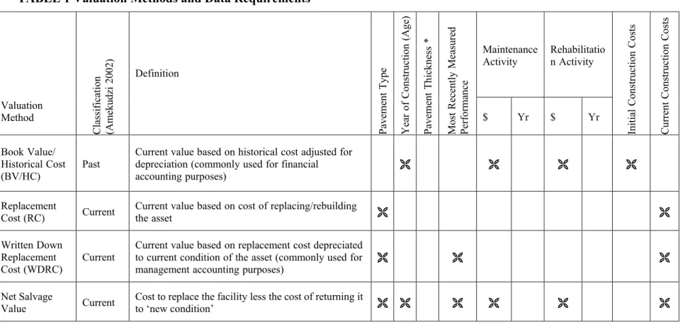
Within the framework of asset management, asset valuation is used to calculate the current and future value. Cowe Falls et al [2004] compared the asset valuation methods summarized in Table 1, using a robust data set from the City of Edmonton. In this

analysis, the asset value was calculated for a base year of 1993 and it was found that asset value varied significantly for each of the methods. Past-based approaches which use historical expenditures to determine value were clearly different to current-based valuation methods that use current data.

Calculating current or past value is relatively straight-forward; the difficulty comes when selecting a valuation method that will be used to project future value using any of the methods. Because of this difficulty, most agencies use current or past based methods for valuation of civil assets. Whatever methodology is used, it must be based upon robust values that can be predicted with some degree of accuracy. If a parameter within the method cannot be predicted into the future with comfortable levels of certainty, as a result of a large statistical variance, the accuracy of future predicted values will be too inaccurate to be of use.

PERFORMANCE MODELS IN ASSET MANAGEMENT

Performance prediction models are used in component management systems (bridge or pavement) to predict the future performance of the asset and to model the

post-rehabilitation performance. The latter use of the models is necessary for calculation of the cost-effectiveness of competing alternatives in the development of optimized, multi-year rehabilitation programs. In asset valuation, the performance models are used to calculate future performance in either a ‘do nothing’ scenario (that is, where the performance and value are predicted assuming no work is done to improve the asset during the forecast period) or after theoretical expenditure (that is, when a feasible alternative is selected usually through the decision trees).

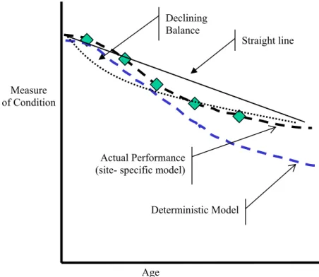
Performance models have been categorized into four basic types: mechanistic, mechanistic – empirical, regression analysis and subjective models [Haas 1994]. In the United States, GASB34 has introduced a fifth performance model based upon financial models, that of straight line depreciation. Straight line depreciation or deterioration models assume that the asset provides equal service to the user for each year of useful life, that is, that the value is consumed at an equal rate per year over the useful life of the asset. It is a simple method that uses the cost to provide the asset minus the salvage value divided by the number of years of expected service. This annual depreciation charge is then deducted from the asset value annually to determine the value. From a performance modeling perspective, the annual depreciation charge is not a dollar value, but rather a reduction in condition. The biggest criticism of straight-line depreciation as a

performance model is that this approach monitors consumption of the asset and does not acknowledge good stewardship of the asset through timely preventive maintenance. Also, all capital assets are assumed to have the same slope and it is difficult to discern

differences in materials, designs etc. That is, it is difficult, if not impossible, to identify over or under performers.

Straight-line depreciation can undervalue or overvalue assets as this approach ties performance to age of the asset only, as illustrated in Figure 1. In this Figure, two types of performance models and two types of depreciation models are presented graphically. Regardless of which model or approach is used, it is necessary to monitor the

performance over time, In other words, it is not possible to model an asset without measurement of its condition, however defined.

THE CITY OF EDMONTON ASSET VALUATION CASE STUDY

The City of Edmonton began implementation of the Municipal Pavement Management Application (MPMA) in 1988 with the first performance data collection survey. From this database, inventory, historical work activities and costs and, performance data for approximately 9,000 road sections were extracted and an analysis data set created using the arterial and collector road sections. Only those sections that have actual data (as opposed to predicted or estimated values) for a defined year were used, creating an analysis set of 113 sections. This is particularly important for the historical rehabilitation and maintenance cost values.

Current Asset Value

The current value for this dataset and the valuation methods listed in Table 1 was discussed in detail in Cowe Falls et al [2004]. Four valuation methods are of particular interest to Canadian agencies because of the current state of the practice. Specifically, Written Down Replacement Cost (WDRC), Replacement Cost (RC), Book

Value/Historical Cost (BV/HC) and Net Salvage Value (NSV) are of interest to the transportation field. Of particular relevance to Canadian agencies are Replacement Cost (RC) and Written Down Replacement Cost (WDRC) which are methods that are used in several Canadian provinces. WDRC is one of the few methods that takes into account engineering deterioration through the use of performance based models. Transport Canada has recently suggested Net Salvage Value, which is equal to the difference between rehabilitation cost and replacement cost, as a method appropriate for valuation of railroads. Given that these are linear assets, Net Salvage Value may have some application for road networks as well. Similar to WDRC, NSV also involves the application of engineering models to the valuation as a decision support system is necessary to develop the rehabilitation costs. In this analysis, two forms of NSV were used: the first (referred to as NSVa) assumed a simple decision tree whereby all road sections that reached a set performance level (equal to a Pavement Distress Index(PDI) of 5.0 on a scale of 0 to 10) were assigned an overlay. The second form (referred to as NSVb) assumed a three level decision tree whereby road sections were assigned crack sealing for PDI = 7.0, a major patch (equal to 10% of the area) for PDI between 6.0 and 6.9 and an overlay for PDI <5.0.

Future Asset Value

Using the three performance models (sigmoidal deterioration, straight-line depreciation with a 1980 horizon and straight-line depreciation with a 25 year horizon set at 1973 for 1999), the condition for each section was projected forward to 1999 (which was assumed to be ‘future value’). Using the projected condition (and remaining service life

determined there from, as applicable) and projected unit costs, the asset value for each section was calculated as well as the total predicted network value.

The 1999 predicted asset values are presented in Table 2. Book Value / Historical Cost remains the highest value and is unchanged from the 1993 value. The difference between past and current based valuations methods is not as clear in the predicted valuation results.

All of the current based methods (WDRC and RC) gained value primarily because of the increase in unit replacement cost during the period. Estimated historical cost will only change if the initial valuation year changes. That is, if the year of first valuation is 1999 rather than 1993, the 1999 replacement cost would be used to estimate historical cost, which would result in a different value.

SENSITIVITY OF VALUE TO PERFORMANCE PREDICTION MODEL

Asset valuation is currently dominated by accounting methods to the chagrin of the engineering community. Accounting practices generally use straight line depreciation for assets, which depreciate value on the basis of age. If depreciation is equated to

deterioration (particularly in the case of the WDRC method), then straight line

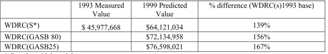
depreciation is an incorrect surrogate for deterioration. Using the GASB34 method as a basis, two depreciation periods are used in the analysis. In the initial implementation instructions GASB 34 set a horizon year of 1980 for the calculation. This year corresponds to the convergence point at which inflation and discount rates results in a zero value when agencies estimate value on the basis of deflated replacement cost. A second method uses a 25 year horizon for valuation, which for the Edmonton data set is equivalent to 1968 (for the current valuation of 1993) or 1973 (for the future valuation of 1999). One of the issues with imposition of a horizon year is that tangible assets, such as pavements and bridges, should not be evaluated on the basis of age or consumption with finite lives, rather engineering-based deterioration should be used to calculate value. The goal of asset management is to maintain condition and consequently value. Sensitivity to performance models is evaluated through a comparison of the straight line valuations (WDRC (80) & (25)1) in Table 3. WDRC for the three models, when compared to the measured WDRC in 1993 is an indication of the variability to be expected in the

performance models. In particular, this provides some indication of the impact of using two models (a financially based straight line model and an engineering based sigmoidal model) to describe the network value.

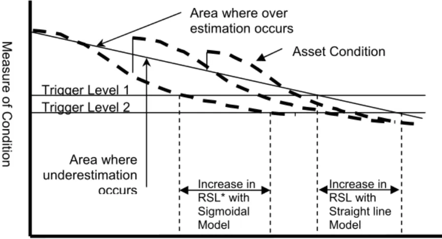
The selection of performance prediction model is important in the discussion of under or over valuation of the network. As shown in Figure 2, straight line depreciation can over or under estimate value at any time during the asset life when compared to performance based deterioration.

SENSITIVITY OF VALUE TO POLICY DECISIONS

Asset value can be defined in terms of the users and owners within the limits of condition, utilization, and functional adequacy. Road assets can become functionally inadequate (because of poor geometrics) or under-utilized (because of construction of a new link) and/or deteriorate through use. All of these reduce the value of the asset to the

1 _{Written Down Replacement Cost was differentiated into three sub-methods to reflect which performance} model was used to predict condition and therefore the amount of reduction in value. These are noted as WDRC(s), WDRC(80) and WDRC(25).

owner and user, but the threshold at which functional adequacy, utilization or deteriorated condition reduce the value (or define needs in terms of required work) is defined by policy makers. Many of the valuation methods include parameters that fall into the realm of policy as summarized in Table 1. The parameters that are defined by policy include the minimum acceptable level or rehabilitation trigger, the alternatives used for

rehabilitation and the decision trees used to select treatments and the remaining service life. Book Value, Replacement Cost and Written Down Replacement Cost do not include parameters that are defined by policy, which means that these three methods are the least sensitive to policy changes. This point is illustrated in Figure 2 where two minimum acceptable levels are plotted on the graph. If an agency lowers the threshold PDI from 6.0 to 5.0, say, there is a consequent increase in the remaining service life and therefore a change in the accumulated depreciation and value for the asset.

REPORTING ASSET VALUE

Based upon the comparative analysis of valuation methods and using a small data set from the City of Edmonton pavement database, the current based methods are the most stable, easiest and simplest methods to use. Replacement Cost (RC) is the easiest method to use as it requires only the area of the network and an average unit construction cost. The difficulty with Replacement Cost is in the prediction of future asset value and the assumption that the asset value is based upon complete replacement of the asset rather than some incremental improvement through asset preservation techniques (a relatively impractical assumption). Written Down Replacement Cost (WDRC) provides an indication of the current deteriorated condition of the asset, and unlike RC, it can be predicted into the future through the use of performance models. As it is based upon Replacement Cost, it too suffers from the inability to accurately predict the future unit. Net Salvage Value (NSV) has some promise because of the incorporation of decision trees into the determination of the rehabilitation cost, but as with both WDRC and RC, it is dependant on the ability to predict the RC into the future as the method is the

difference between replacement and rehabilitation costs.

Public reporting of asset value should include asset condition and, as it is a performance measure, it should also provide some indication of asset management in terms of improved or maintained condition. Sound asset management will result in retained value; poor asset management will result in lost value. When reporting asset value to the public and/or senior decision makers, a combination of valuation methods can be used, for example, the Replacement Cost and Written Down Replacement Cost can be reported. In the City of Edmonton pavement analysis set, the RC for 1993 is $81 million, while the WDRC is $46 million, indicating a loss of value of 57% because of deteriorated condition. Reporting both values provides some indication of whether the City is falling behind or keeping abreast of infrastructure deterioration in a manner that is more understandable to the public than reporting Pavement Distress Index.

Differential Value is the Key

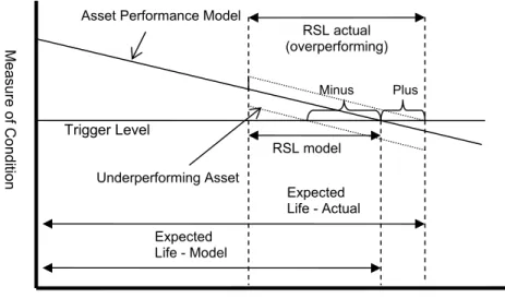
Regardless of which method is used to establish the initial value for the network, the key will be maintenance of that value through timely and appropriate asset preservation and as such it is important to measure the change in value year over year. To do that, a stable measure that has minimal fluctuations due to data variability, policy changes and/or market forces is required. One approach is to measure and report the differential

value rather than the actual value using an Asset Service Index (ASI). This index would measure deviations from the expected value as a result of neglect, action and/or changes in usage which could accelerate or decelerate deterioration. Using a differential from the expected, the asset service index would be reported as a plus/minus value with a plus value indicating over-performing and a minus indicating under-performing as illustrated in Figure 3. The condition is converted to a remaining service life (by comparison to either the predicted point when the condition reaches a minimum acceptable level or age and adjusted by the replacement cost. Using replacement cost to adjust the asset service index indicates the amortized cost of the net salvage value (which is the difference between the replacement cost and rehabilitation cost). Using the concept of an asset service index that compares the expected condition to the measured condition could be calculated using the following equation2 :

Asset Service Index = ((Replacement Cost)*Remaining Service Life/Expected Life)actual - ((Replacement Cost)*Remaining Service Life/Expected Life)model

As seen in Figure 3, an improvement in asset condition as a result of maintenance will result in an increase in the Remaining Service Life (RSL) as well as the expected life and this will result in a positive value.

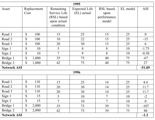
Similarly, accelerated deterioration will result in a decrease in RSL which will translate into a negative value. Asset Service Index (ASI) uses any form of model (straight line or sigmoidal) and is index scale independent. Expected Life is determined from the design life, which can vary from 100 years for bridges to 10 years for signs and roadside furniture. The Remaining Service Life is determined by the condition and the performance model. An example is presented in Table 4 below, where the ASI for three asset types (roads, bridge and signs) is calculated for two years. RSL actual is calculated from the condition of the asset in that year and the projected number of years until rehabilitation is required. The RSL model is the expected RSL based upon the

performance model and indicates whether the asset is in better than expected or worse than expected condition. The replacement costs vary from asset to asset and change (in this case, increase) from year to year. In 1995, the replacement costs are $100, $10 and $1,000 per unit or square metre. Road 3 and Bridge 2 are both in better than expected condition and as such have a positive ASI, while all other assets in 1995 are in a negative position. The total network ASI is negative which indicates a network that has not been appropriately preserved through good asset management practices and/or is under-funded. In the next valuation year the ASI deficit decreases (from -51.05 to -1.2) even though the replacement cost for all asset types increases. Using RC or WDRC this might not be the case given the results of the Edmonton analysis dataset. This increase in ASI is due largely because of the increased RSL of Road 2 (due to a major maintenance activity) and retention of RSL for the other assets because of appropriate maintenance.

The objective of ASI is to maintain a value as close to 0 as possible with most of the sections having a positive (i.e., over-performing) value. There are several advantages to this approach including scale independence, the ability to use multiple model types (for example, signs can be straight line, while pavements can be sigmoidal), and the lack of

sensitivity to replacement cost. Exploration of the potential for Asset Service Index is an area for future research.

A PROPOSED ASSET VALUATION FRAMEWORK

As discussed in this paper, asset value can be calculated using several valuation methods for a pavement network and this can be extended to other asset categories within the highway right of way. The selection of which method for which asset depends on data stability, consistency and availability, as well as the ability to accurately predict those data into the future. An implementation framework is needed that addresses not only such issues as appropriate methods for each asset category, but also how to satisfy the needs of both financial and management reporting in terms of horizon year and frequency of reporting.

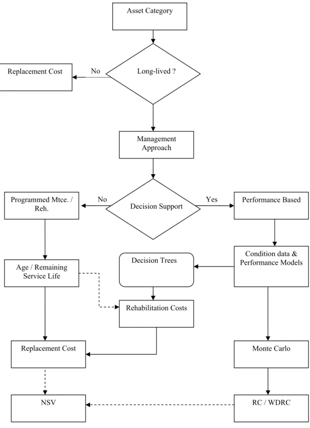
Using the FHWA protocol for Life Cycle Cost Analysis (LCCA) where assets above a threshold value must use LCCA during project selection, as an example, a framework is proposed in Figure 4 that provides guidance to managers in selecting the valuation

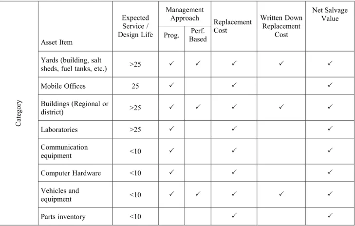
approach based upon asset useful life, management approach, and data availability. Assets that are short lived and/or are managed using a programmed maintenance and/or rehabilitation approach are valued using Replacement Cost (RC). Assets that have long lives and performance models can use Written Down Replacement (WDRC). Using this framework, assets owned by highway agencies have been summarized in Table 6 (after (6)). Each of these asset categories can use Replacement Cost, and/or Written Down Replacement Cost as suitable valuation methods and they have been screened according to expected life and management approach. All assets that have performance models and long lives, should be valued using WDRC; shorter lived assets or those managed by programmed maintenance / rehabilitation can be valued with RC.

CONCLUSION

Total network asset value has been calculated for several valuation methods using a subset of the City of Edmonton arterial and collector network. Using real, not extrapolated, historical costs, the Book Value, Written Down Replacement Cost,

Replacement Cost and Net Salvage Value methods produced large variations in total and mean asset value for the network. Book Value produced the highest total network value, primarily because of the inclusion of historical construction cost and accumulated

rehabilitation and maintenance costs.

Book Value was found to have the highest value, while Written Down Replacement Cost produced the lowest value. Also, the historically based methods produced higher total and mean values than the current based methods. Edmonton has experienced cycles of boom and bust and in the boom times high unit costs are reflected in the network through a relatively large portion of the network being built at very high unit costs. When using historical values there is a potential for wide distortion in the values and this is borne out by the range and variance of all of the values calculated using historical values.

Current based methods, using replacement cost, have lower variability and produce lower values which can be interpreted as providing greater stability from year-to-year. Agencies that are in the process of calculating asset values should also recognize that despite the variability in the method, what really is important is the change over time of the asset being valued. As asset valuation has the potential to become a performance measure or indicator, it is important that agencies be able to report how well they are

retaining asset value as a result of proper management. One approach would be to report the Replacement Cost and the Written Down Replacement Cost. The former indicates the cost to replace the asset and the latter provides an indication of how well the asset is being managed. WDRC also incorporates engineering performance models and

recognizes good management rather than consumption as in the case of straight line depreciation (used in GASB). The difference between RC and WDRC should not change if proper management of the asset is in place, whereas an increase in the difference would indicate that the network is losing value.

Working with the concept that asset value should be reported as a differential, the Asset Service Index (ASI) was presented for consideration. ASI uses the specific performance model of the asset category and replacement cost to calculate a single index that can be used to develop optimized multi-year programs for complex assets.

Regardless of which valuation method is used, the important point is to select a valuation method that can be easily sustained and managed, is not data and/or analytically burdensome and that proper asset management should result in retention of asset value. What matters most is the change in the asset over time and proper management will preserve asset value.

REFERENCES:

1. [Cowe Falls and Haas 2001] Cowe Falls, Lynne and Ralph Haas, Measuringand Reporting Highway Asset Value, Condition and Performance, Transportation

Association of Canada, 2001

2. [Cowe Falls, Haas and Tighe 2004] Cowe Falls, Lynne, Ralph Haas and Susan Tighe, “Comparison of Asset Valuation Methods” Transportation Association of Canada, 2004

3. [TRB 2002] Minutes of the TRB Asset Management Task Force (AT150) annual meeting, January 2002 Washington, D.C.

4. [Amekudzi 2002] Amekudzi, A., Herabat, P., Wang, S. and Lancaster, C. 2002, “Multipurpose Asset Valuation for Civil Infrastructure: Transportation Research Record 1812, TRB, National Research Council, Washington D.C. 211 - 218 5. [GASB 1999] “Statement No. 34 of the Governmental Accounting Standard

Board. Basic Financial Statements and Management’s Discussion and Analysis for State and Local Governments” Governmental Accounting Standard Series, No. 171-A, Governmental Accounting Standards Board, June, 1999.

6. [Haas et al 1994] Haas, Ralph, W. Ronald Hudson and John Zaniewski, Modern Pavement Management, Krieger Publishing Company, Malabar, 1994

7. [Haas and Raymond 1999a] Haas, Ralph and Chris Raymond, “Asset

Management for Roads and Other Infrastructure”, Paper Presented to Annual Asphalt Seminar, Ontario Hot Mix Producers Assoc., Toronto, December 1999

TABLE 1 Valuation Methods and Data Requirements

Maintenance

Activity RehabilitationActivity

Valuation Method Classification (Amekud zi 200 2) Definition Paveme nt Ty pe Year of C onstruction (A ge ) Paveme nt T hickne ss * Mo st Recently Measure d Performa nce $ Yr $ Yr Initial C onst ru ction Co sts Cu rr en t Construction Co st s BookValue/ HistoricalCost (BV/HC) Past

Currentvaluebasedonhistoricalcostadjustedfor depreciation(commonlyusedforfinancial accountingpurposes)

Replacement

Cost(RC) Current Currenttheasset valuebasedoncostofreplacing/rebuilding WrittenDown

Replacement

Cost(WDRC) Current

Currentvaluebasedonreplacementcostdepreciated tocurrentconditionoftheasset(commonlyusedfor managementaccountingpurposes)

Net Salvage

TABLE 2 Total Network Value for Predicted and Measured Value (sorted by 1999 Measured Value)

Difference between Predicted and Measured

1999 Valuation Method 1999 Predicted _Value 1999 Measured _Value

Current / Past Based (absolute) % WDRC(S) $64,121,034 $52,812,542 Current $11,308,492 21% NSVb $91,980,731 $71,940,515 Current $20,040,216 28% NSVa $104,002,295 $95,661,599 Current $8,340,696 9% RC $113,525,224 $105,184,529 Current $8,340,695 8% BV/HC $154,692,968 $154,692,968 Past $0 0%

TABLE 3 Comparison of Performance Models on Valuation

1993 Measured

Value 1999 Predicted Value % difference (WDRC(s)1993 base)

WDRC(S*) _{$ 45,977,668 $64,121,034} 139%

WDRC(GASB80) $72,134,958 156%

WDRC(GASB25) $76,598,021 167%

TABLE 4 Asset Service Index

1995 Asset Replacement

Cost ServiceRemainingLife (RSL)based uponactual

condition

ExpectedLife

(EL)actual RSLuponbased performance model ELmodel ASI Road1 $ 100 15 25 15 25 0 Road2 $ 100 10 22 15 25 -15 Road3 $ 100 20 30 15 25 6 Sign1 $ 10 5 8 8 10 -1.75 Sign2 $ 10 7 9 8 10 -0.30 Bridge1 $ 1,000 35 75 40 75 -67 Bridge2 $ 1,000 42 75 40 75 27 Network ASI -51.05 1996 Road1 $ 110 15 25 14 25 4.4 Road2 $ 110 20 30 14 25 11.7 Road3 $ 110 20 30 14 25 11.7 Sign1 $ 15 5 10 7 10 -2 Sign2 $ 15 7 10 7 10 0 Bridge1 $ 2,000 35 75 39 75 -107 Bridge2 $ 2,000 42 75 39 75 80 Network ASI -1.2

TABLE 5 Sensitivity of Valuation Method to Policy Decisions

Method Parameters Subject to Policy Decisions Written Down

Replacement Cost

•

Replacement Cost

•

GASB 34

•

TABLE 6 Asset Valuation Methods (6)

Management Approach Category AssetItem ExpectedService/

DesignLife Prog. Perf. Based Replacement Cost WrittenDown Replacement Cost Net Salvage Value Pavement 25 _{3 3 3 3 3} Bridges >25 _{3 3 3 3 3} DrainageStructures (e.g.StormSewers)

>25 _{3 3 3 3 3}

Grade(cut/fill) >25 _{3 3 3}

Signs <25 _{3 3 3}

Signals&loop

detectors <25 3 3 3

FTMSCameras _<25

3 3 3

Guiderails&barrier

walls 25 3 3 3 3 3

Fences&noise barriers

25 _{3 3 3 3 3}

Culverts >25 _{3 3 3}

Pavementmarkings _{<25 3 3 3}

Lighting 25 _{3 3 3}

Sidewalks&bike paths

25 _{3 3 3 3 3}

Curbs&gutters 25 _{3 3 3 3 3}

Utilities(cable,gas,

hydro,phone,water) >25 3 3 3

Fixed Assets (W ith in the Right of Wa y)

Weighscales&

TABLE 6 Asset Valuation Methods (cont’d) Management Approach AssetItem Expected Service/

DesignLife Prog. _Based Perf.

Replacement Cost WrittenDown Replacement Cost Net Salvage Value

Yards(building,salt

sheds,fueltanks,etc.) >25 3 3 3 3 3

MobileOffices 25 3 3 3 Buildings(Regionalor district) >25 3 3 3 3 3 Laboratories >25 3 3 3 Communication equipment <10 3 3 3 ComputerHardware <10 3 3 3 Vehiclesand equipment <10 3 3 3 3 3 Categ ory Partsinventory <10 3 3

FIGURE 1 Performance Prediction Models

Actual Performance (site- specific model)

Deterministic Model Measure of Condition Age Declining Balance Straight line

Figure 2 Over or Under Estimation of Asset Condition Relative to Performance Models Trigger Level 1 Trigger Level 2 Increase in RSL* with Sigmoidal Model Increase in RSL with Straight line Model Measur e of Co nditi on

Time RSL= Remaining Service Life

Area where underestimation occurs

Area where over estimation occurs

FIGURE 3 Asset Service Index Concept Expected Life - Model Trigger Level RSL model Expected Life - Actual Measur e of Co nditi on Time RSL actual (overperforming) Asset Performance Model

Underperforming Asset

Plus Minus

Figure 4 Implementation Framework for Asset Valuation Method Selection Replacement Cost Asset Category Management Approach Rehabilitation Costs Performance Based

Condition data & Performance Models Programmed Mtce. / Reh. Age / Remaining Service Life Replacement Cost NSV RC / WDRC No Decision Support Long-lived ? No Yes Monte Carlo Decision Trees