Unsupervised deep learning research and implementation of variational autoencoders

Degree in Telecommunication Technologies Engineering

2017-2018

Bachelor Thesis

Unsupervised Deep Learning

Research and Implementation of Variational Autoencoders

Pablo Sánchez Martín

Supervised by

Pablo Martínez Olmos

Leganés, June 2018

This work is licensed under a Creative Commons Attribution-Noncommercial-No-DerivativeLicense.

Abstract

Generative models have been one of the major research fields in unsupervised deep learning during the last years. They are achieving promising results in learning the distri-bution of multidimensional variables as well as in finding meaningful hidden representa-tions in data.

The aim of this thesis is to gain a sound understanding of generative models through a profound study of one of the most promising and widely used generative models family, the variational autoencoders. In particular, the performance of the standard variational autoencoder (known as VAE) and the Gaussian Mixture variational autoencoder (called GMVAE) is assessed. First, the mathematical and probabilistic basis of both models is presented. Then, the models are implemented in Python using the Tensorflow framework. The source code is freely available and documented in a personal GitHub repository cre-ated for this thesis. Later, the performance of the implemented models is appraised in terms of generative capabilities and interpretability of the hidden representation of the inputs. Two real datasets are used during the experiments, the MNIST and "Frey faces". Results show the models implemented work correctly, and they also show the GMVAE outweighs the performance of the standard VAE, as expected.

Keywords: deep learning, generative model, variational autoencoder, Monte Carlo simulation, latent variable, KL divergence, ELBO.

ACKNOWLEDGEMENTS

To start with, I would like to thank my family, for being completely supportive through-out the time I have been conducting this thesis and the degree. I would like to thank spe-cially my parents for helping me on a daily basis, both on the good and bad times, for teaching me important principles such as perseverance and basically, for everything they do.

I would also like to thank my university colleagues with which I have shared unfor-gettable memories during the last years.

Last but not least, I would like to thank my supervisor Pablo M. Olmos. I am ex-tremely grateful to him for the time he has invested in teaching me everything this thesis required, in resolving any issue that arose and for being such a good mentor.

CONTENTS

2.1. Overview of Generative Models . . . 7

2.1.1. Explicit Density Models . . . 8

2.1.2. Implicit Density Models . . . 8

2.2. Probabilistic PCA . . . 9

2.3. Neural Networks . . . 11

2.3.1. Convolutional Neural Networks . . . 12

3. VARIATIONAL AUTOENCODER . . . 14

3.1. Overview . . . 14

3.2. Objective . . . 16

3.2.1. Dealing with the Integral overz . . . 16

3.2.2. Inference Network: qϕ(z|x) . . . 17 3.2.3. KL Divergence . . . 17 3.2.4. Core Equation . . . 18 3.2.5. ELBO Optimization . . . 19 3.2.6. Reparameterization Trick . . . 21 3.3. Sampling . . . 21

4. GAUSISIAN MIXTURE VARIATIONAL AUTOENCODER . . . 22 4.1. Introduction. . . 22 4.2. Overview . . . 22 4.3. Definingzdirectly as a GMM . . . 23 4.4. Optimization Function . . . 23 4.4.1. Reconstruction Term . . . 25

4.4.2. Conditional prior term . . . 25

4.4.3. W-prior term . . . 26 4.4.4. Y-prior term. . . 26 4.4.5. ELBO Equation . . . 26 4.5. Reparameterization Trick . . . 27 4.6. Sampling . . . 27 5. METHODOLOGY . . . 28 5.1. Objective . . . 28 5.2. Prepare Data . . . 28 5.3. Model Architecture . . . 29 5.4. Definition of hyperparameters . . . 29 5.5. Experimental Setup . . . 30

5.6. GMAVE numerical stability. . . 32

5.6.1. Approximation of pβ(yj =1|w,z) . . . 32

5.6.2. Output restrictions . . . 33

5.7. Motivate clustering behaviour. . . 34

5.8. Metrics . . . 34

5.9. Visualization of results. . . 35

6. RESULTS . . . 37

6.1. Initial considerations . . . 37

6.2. Experiment 1: VAE . . . 37

6.3. Experiment 2: Understanding the latent variables of GMVAE . . . 39

6.4. Experiment 3: Comparison between GMVAE and VAE . . . 40

6.5. Experiment 4: Performance evaluation with corrupted input. . . 42

7. SOCIO-ECONOMIC ENVIRONMENT . . . 46 7.1. Budget. . . 46 7.2. Practical Applications . . . 47 8. CONCLUSIONS . . . 49 8.1. Conclusions. . . 49 8.2. Future work . . . 50

A. VAE LOSS RESULTS . . . 51

B. GENERATED SAMPLES . . . 52

C. KL DIVERGENCE OF GMM. . . 53

D. GMVAE OBJECTIVE FUNCTION DERIVATIONS. . . 54

D.1. Conditional prior term. . . 54

D.2. W-prior term . . . 55

D.3. Y-prior term . . . 55

LIST OF FIGURES

1.1 Several samples from the MNIST dataset. . . 2

1.2 Several samples from Frey faces dataset. . . 3

2.1 Taxonomy of generative models based on maximum likelihood. Extracted from [11]. . . 8

2.2 PCA generative model. Extracted from [18]. . . 10

2.3 Mathematical model of a simple artificial neuron. . . 11

2.4 Several activation functions. . . 12

2.5 Edge detector kernel. Extracted from [26]. . . 13

2.6 Simple CNN Architecture. . . 13

3.1 Probabilistic view of VAE. Extracted from [29]. . . 15

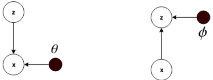
3.2 Graphical models for the VAE showing the generative model (left) and the inference model (right). . . 15

4.1 Graphical models for the GMVAE showing the generative model (left) and the inference model (right). . . 22

5.1 Data diagram. . . 28

6.1 Example of good clustering but poor generation result. . . 38

6.2 Example of poor clustering but good generation result. . . 39

6.3 Examples of PCA latent space representation and reconstruction varying dimz. . . 39

6.4 Scatter plot of variablew. . . 40

6.5 Scatter plot of variable z. . . 40

6.6 Example of bad clustering but good generation result. . . 41

6.7 Example of good clustering and good generation result. . . 42

6.8 Reconstruction without noise. . . 43

6.9 Reconstruction with uniform noise. . . 43

6.10 Reconstruction with dropout noise. . . 43

6.12 Example of results using VAE convolutional architecture on MNIST. Model (a) and (b) with dimz=2 and model (c) and (d) with dimz=10. . . 45 6.13 Example of results using GMVAE’s convolutional architecture on FREY

dataset. . . 45 B.1 Low quality generated samples with different VAE configurations. . . 52

LIST OF TABLES

6.1 Loss results of the best clustering configurations. Ordered by ValidLoss. . 38

6.2 Loss results of the best generative configurations. Ordered by KLloss. . . 38

6.3 Best clustering configurations of VAE in GMVAE. Ordered by CondPrior. 41 6.4 The best generative configurations of VAE in GMVAE. Ordered by Cond-Prior. . . 41

6.5 Loglikelihood results. . . 43

6.6 GMVAE training result. . . 44

6.7 VAE training result. . . 44

7.1 Detailed budget. . . 47

1. INTRODUCTION

This chapter presents the project in brief. It contains the motivation and objectives of this thesis, the regulatory framework related to the project, the requirements, the activities undertaken and the overall structure of the document.

1.1. Statement of Purpose

Neural networks have existed since the definition of the Perceptron in 1958 [1]. How-ever, they did not become popular until the appearance of backpropagation in the late 80s [2]. Latest advances in distributed computing, specialized hardware and an exponential growth in the amount of data created, have enabled to train extremely complex neural net-works with large number of layers and parameters. The discipline that studies this type of networks is known as Deep Learning and it is achieving state-of-the-art results in many difficult problems such as speech recognition [3], object detection [4], text generation [5] and recently in data generation.

A generative model is a kind of unsupervised learning model that aims to learn any type of data distribution and it has the potential to unveil underlying structure in the data. Generative models have recently emerged as a revolution in deep learning with many applications in a wide-ranging variety of fields such as medicine, art, gaming or self-driving. Deep learning, and specially generative models, is evolving so fast that it is difficult to keep up with the latest developments.

For these reasons, the purpose of this work is to serve as a sound introduction to deep learning generative models. To achieve this goal, the variational autoencoder model or VAE, one of the most widely used generative models, is studied in detail and compared to one of its variations: the Gaussian Mixture VAE. The implementation of the GMVAE will be based on [6] with some modifications proposed in this work. So the main objective of this bachelor thesis can be expanded as follows:

1. Study in detail the mathematical and probabilistic basis of the variational autoen-coders.

2. Explore dimesionality reduction algorithms.

3. Master Tensorflow, a widely used deep learning library for python. 4. Implement the VAE and GMVAE models using different architectures. 5. Compare and evaluate the algorithms implemented for different datasets.

As it will be seen further on, the GMVAE describes a two level hierarchical latent space that aims to capture the multimodal nature of the input data. Due to this, the hy-pothesis of this thesis is that the GMVAE model improves the generative and clustering capabilities of the standard VAE. Experiments will be conducted to test this hypothesis.

1.2. Requirements

The first part of this thesis is purely theoretical. In the second part, the following tools are required for the implementation of the models: datasets, programming framework and GPU power.

1.2.1. Datasets

The datasets used for this thesis are the MNIST and "Frey faces" (or FREY) datasets, both publicly available. They consist of images with dimensionDxthat represents the number

of pixels:

MNIST:Dx = 28x28=784

FREY:Dx =20x28= 560

MNIST Dataset

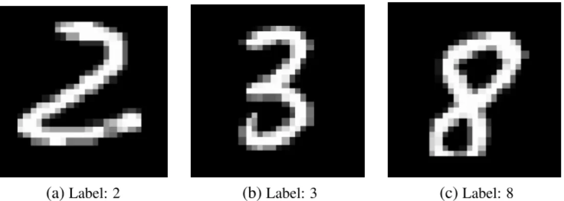
The MNIST database [7] is a labeled collection of gray-scale handwritten digits dis-tributed by Yann Lecun’s website. Each image is formed by 28x28 size-normalized pix-els. The MNIST database is often used to assess performance of algorithms in research. There are functions available to prepare the dataset so there is no need to write code about preprocessing or formatting.

(a)Label: 2 (b)Label: 3 (c)Label: 8 Fig. 1.1. Several samples from the MNIST dataset.

FREY Dataset

The "Fray faces" or FREY dataset [8] consists of 1965 images with 20x28 pixels of Bren-dan’s face taken from sequential frames of a video. Although this is an unlabeled dataset, Brendan appears varying the expressions of his face thus showing different emotions, such as happiness, anger or sorrow, that can be associated to different classes. Several samples are shown in figure 1.2.

(a)Label: Happy (b)Label: Sad (c)Label: Angry Fig. 1.2. Several samples from Frey faces dataset.

1.2.2. Programming Framework

Python was the programming language chosen to implement the models and run the ex-periments. Python makes extremely easy to inspect variables and outputs, to debug code and to visualize results. Moreover, there are great tools and software packages for deep learning available in this programming language such as Keras, Theano, TensorFlow or Caffe. In particular, Tensorflow has been used in this thesis.

Tensorflow is an open-source software library developed by Google Brain for internal use. It was released under the Apache 2.0 open source license on November 2015. It provides much control over the implementation and training of neural networks. More-over, it comes with a wonderful suite of visualization tools known as TensorBoard that allows visualizing TensorFlow graphs, plot the values of tensors during training, visualize embeddings (using T-SNE and PCA algorithms) and much more.

For all these reasons, TensorFlow was the choice to develop this project.

1.2.3. GPU Power

To speed up the training process, the graphic card NVidia GeForce GTX 730 GPU of a personal computer was used to train the models. To utilize the graphic cards of the computer, the GPU implementation of Tensorflow was used. This led to great reduction in training time compared to using the CPU Tensorflow operation mode. However, as the complexity of the models increased, the simulations needed more computational power

to be completed on a reasonable amount of time. Thus, they were launched in the servers of the Signal Processing Group.

1.3. Regulatory Framework

This section discusses the legislation applicable to the realization of this bachelor thesis, namely the development of generative models and the use of personal data. The protection of intellectual property is also presented.

1.3.1. Legislation

Data is an essential tool to train any kind of machine or deep learning algorithm and its quality can condition the resulting model. In some cases the data required is freely available and completely anonymous, for example the MNIST dataset. However, in many other cases the data needed is obtained from users, for example data regarding localiza-tion, gender, age or personal interests, and therefore it is necessary to take into account aspects such as privacy, security and ethical responsibility.

On 25th May it came into force in the European Union the General Data Protection Regulation (GDPR) [9], which aims to protect individuals’ personal information across the European Union. This new regulation applies to business that somehow use personal data. In short, the GDPR expands the accountability requirements to use personal data, substantially increases the penalties for organizations that do not comply with this regu-lation and it enables individuals to better control their personal data. The following are the key changings of the GDPR but notice the full document contains 11 chapters and 99 articles:

• Harmonized regularization across the EU.

• Organizations can be fined up to e20 million or 4% of the entity’s global gross revenue.

• The individual must clearly consent the use of their personal data by means of "any freely given, specific, informed and unambiguous indication" and this consent must be demonstrable.

• More specific definition of personal data: any direct or indirect information relating to an identified or identifiable natural person.

• Data subjects rights: breach notification, right to be forgotten, access to data col-lected, data portability, privacy by design and data protection offices.

It is also important to mention that software is a type of Intellectual Property (IP). Therefore, according to the Article I of Spanish Royal Legislative Decree [10], it can be protected by means of copyright, patents or registered trademarks.

1.4. Work Plan

All the activities realized during this bachelor thesis can be grouped in six blocks, as shown in Table 1.1.

Project Documentation Planification and writing of final report. Document source code in GitHub

Research Search for papers and articles explaining variational

autoen-coders and dimensionality reduction algorithms

Datasets selection Download and test datasets.

Software and hardware selec-tion

Select programming language, deep learning libraries and estimate computation power needed.

Implementation and experi-mentation

Implement the models and conduct the experiments. Documents hand-in and

pre-sentation

Upload thesis memory and deliver the presentation.

Table 1.1. Work packages.

1.5. Organization

In addition to the introductory chapter, this work contains the following chapters:

• Chapter 2,Background, presents the theoretical concepts needed to understand the variational autoencoder and to conduct the experiments along with an overview of generative models.

• Chapter 3,Variational Autoencoder, explains in detail the VAE model, describing its architecture and the loss function used for training.

• Chapter 4,Gaussian Mixture VAE, explains in detail the GMVAE model, describing its architecture and the loss function used for training.

• Chapter 5, Methodology, presents a description of the experiments realized and some important aspects about the implementation of the models.

• Chapter 6,Results, shows and explains the results obtained.

• Chapter 7, Socio-economic environment, presents some possible practical applica-tions of the study conducted in this work and the socio-economic impact they can generate.

• Chapter 8,Conclusions, discusses the results obtained and states the conclusions of the thesis.

• Appendix A, VAE loss results, contains a table with all the loss values of the con-figurations tested.

• Appendix B,Generated samples, contains generated samples of VAE.

• Appendix C, KL Divergence of GMM, explains why the Kullback-Leibler diver-gence is intractable when Gaussian mixture models are involved.

• Appendix D,GMVAE Objective Function Derivations, explains all the intermediate steps needed to obtain the loss function of the GMVAE model.

2. BACKGROUND

In this section, the theoretical concepts required to understand the VAE are explained. First, a review of the current situation of generative models is presented. Then, the Prob-abilistic PCA is explained as this algorithm can be understood as a simplified form of the VAE. Thus, this section serves as an introduction to the model in study. Later, a brief introduction of neural networks is made. Finally, a summary of convolutional neural networks, which are really efficient when working with images, is also presented.

2.1. Overview of Generative Models

Generative models are classified as unsupervised learning. In a very general way, a gener-ative model is one that given a number of samples (training set) drawn from a distribution

p(x), is capable of learning an estimate pg(x) of such distribution somehow.

There are several estimation methods on which generative models are based. How-ever, to simplify their classification [11], only generative models based on maximum likelihood will be considered.

The idea behind the maximum likelihood framework lies in modeling the approxima-tion of the prior distribuapproxima-tion of the data, which is known as the likelihood, through some parametersθ: pθ(x). Then the parameters that maximize the likelihood will be selected.

θ∗₌ arg max θ N ∏ i=1 pθ(x(i)) (2.1)

In practice, it is typical to maximize the log likelihood logpθ(x(i)) as it is less likely to suffer numeric instability when implemented on a computer.

θ∗₌ arg max θ N ∑ i=1 logpθ(x(i)) (2.2)

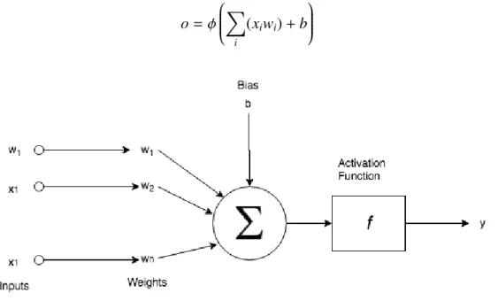
If only generative models based on maximum likelihood are considered , they can be classified in two groups according to how they calculate the likelihood (or an approxima-tion of it): explicit density models or implicit density models. The whole taxonomy tree is shown in figure 2.1.

Fig. 2.1. Taxonomy of generative models based on maximum likelihood. Extracted from [11].

2.1.1. Explicit Density Models

Explicit density models can be subdivided in two types: those capable of directly maxi-mizing an explicit density pθ(x) and those capable of maximizing an approximation of it. This subdivision represents two different ways of dealing with the problem of tractabil-ity when maximizing the likelihood. Some of the most famous approaches to tractable density models are Pixel Recurrent Neural Networks (PixelRNN) [12] and Nonlinear In-dependent Components Analysis (NICA) [13].

The models that maximize an approximation of the density functionpθ(x) are likewise subdivided into two categories depending on whether the approximation is deterministic or stochastic: variational or Markov chain. Later in this work the most widely approach to variational learning, the variational autoencoder also known as VAE will be analyzed in detail (see Chapter 3 and Chapter 4).

Furthermore, Section 2.2 describes one of the simplest explicit density models, Prob-abilistic PCA, and serves as an introduction to this type of models.

2.1.2. Implicit Density Models

These are models that do not estimate the density probability but instead define a stochas-tic procedure which directly generates data [14]. This procedure involves comparing real data with generated data. Some of the most famous approaches are the Generative Stochastic Network [15] and Generative Adversarial Network [16].

2.2. Probabilistic PCA

Principal Component Analysis (known as PCA) [17] is a technique used for dimension-ality reduction, lossy data compression and data visualization that has wide-ranging ap-plications in fields such as signal processing, mechanical engineering or data analysis. Depending on the field scope, it can also be named discrete Karthunen-Loéve transform.

PCA is a technique that can be analyzed from two different points of view: linear algebra and probability. In this section it is presented an overview of PCA from the probabilistic point of view as it is closely related to the simplest case of the variational autoencoder and a good starting point to latent variable models. The explanation is largely based on Bishop’s book [18].

Although PCA was firstly conceived by Karl Pearson in 1901 [19], it was not until the late 90s when probabilistic PCA was formulated by Tipping and Bishop [20] and by Roweis [21]. Probabilistic PCA holds several advantages compared to conventional PCA. One of them is that it can be used as a simple generative model and this is why this algorithm is meaningful in this work.

As its name states, PCA finds the principal components of data, or in other words, it finds the features, the directions where there is the most variance. So given a dataset

X = {x(i)_}N

1 with dimensionality Dx, the main idea behind PCA is to obtain a subspace

(called the principal-component subspace) with dimensionDz, being Dz << Dx, so that

each x(i) _{is represented with a z}(i) _{(latent variable) in the best possible way. Then, it is}

possible to recoverx(i)_{from z}(i)_.

x(i)∈ ℜDx _{→ z}(i) _{∈ ℜ}Dz

The probabilistic PCA is a maximum likelihood solution of a probabilistic latent vari-able model in which all marginal and conditional distributions are Gaussian. The likeli-hood function to be maximized is expressed as:

p(x)=

∫

p(x|z)p(z)dz (2.3)

As all distributions are Gaussian, the probability distribution of x can be expressed as p(x) = N(x|µ,C) where the covariance matrix is C = WWT + σ2_{. Therefore, the}

parameters of the model are theDxxDz matrixW , the Dx dimensional vectorµand the

scalarσ2_.

The optimal values of the parameters are obtained using Maximum Likelihood Esti-mation (MLE), maximizing the log-likelihood logp(x).

logp(x|W,µ, σ2)=

N ∑

i=1

=−DxN 2 log(2π)− N 2 log(|C|)− 1 2 N ∑ i=1 (x(i)−µ)TC−1(x(i)−µ)

The optimization can be computed in a closed form [18] or using the EM algorithm [22]. By closed form, the derivative of logp(x|W,µ, σ2_{) with respect to each parameter is}

computed and equal to 0 to obtain the optimal values, namelyµ_ML,WML andσ2_ML.

The optimal meanµ_MLis the sample mean of the data:

µ_ML =

N ∑

i=

x(i)= x¯ (2.4)

The expression for the optimal matrix W shown in equation 2.5 is quite complex. However, all the matrices involved are known or can be obtained. The matrixUM (with

shape Dx x Dz) contains the eigenvectors of the data covariance matrix S which

cor-respond to the largest eigenvaluesλi. These eigenvalues form the diagonal matrix LM,

which has shapeDz xDz. The matrix R(with shapeDz xDz) is an arbitrary orthogonal

matrix.

WML = UM(LM−σ2I)(1/2)R (2.5)

Theσ2_ML represents the average variance associated with the discarded dimensions.

σ2 ML = 1 Dx−Dz Dx ∑ i=Dz+1 λi (2.6)

Now that all the parameters involved are defined and it is known how to compute them, it is possible to define how new samples are generated.

The generation phase comprises two steps. First, the variablezis sample from a priori known distributionp(z). Then, new data samples are drawn fromp(x|z)=N(x|µ(z), σ2I) whereµ(z)=W z+µ. This process is shown in figure 2.2.

Fig. 2.2. PCA generative model. Extracted from [18].

This is a simple case of a generative model where the relation between the latent and the predictive variables is linear:

x∼W z+µ+ϵ

2.3. Neural Networks

Artificial neural networks are a set of machine learning algorithms that simulates the functioning of biological neurons by means of a mathematical model.

Basically an artificial neuron consists of a set of inputsxithat are multiplied by weight

parameterswiand added point wise. Then the bias parameterbis added. Finally, the result

is introduced into a non-linear function, known as activation function, to obtain the output of the neuron. This mathematical model is shown in figure 2.3 and expressed in equation 2.7. o= ϕ ⎛ ⎜ ⎜ ⎜ ⎜ ⎜ ⎝ ∑ i (xiwi)+b ⎞ ⎟ ⎟ ⎟ ⎟ ⎟ ⎠ (2.7)

Fig. 2.3. Mathematical model of a simple artificial neuron.

Activation functions (ϕ) are a remarkably important characteristic of neural networks. They determine whether a neuron should be activated or not and the range of possible outputs. In other words, they determine how and how much information flows through the network. There are several functions that can be used as activation functions. The most common ones are identity, ReLU, Leaky ReLU, sigmoid, tahn and softmax. Some of them are shown below in figure 2.4

(a)Sigmoid (b)Tanh (c)ReLU Fig. 2.4. Several activation functions.

Among them, the Rectifier Linear Unit or ReLU (Equation 2.8) is probably the most widely used function today. It has proven to help to prevent vanishing gradient among other benefits. However, the selection of the activation function depends on the applica-tion.

ϕ(x)=max(0,x) (2.8)

Now that all the basic elements of a neural network are described, the question that arise is how to build a neural network. The process is quite simple: one or several neurons form a layer and several stacked layers form a basic neural network. This is probably the most generic architecture of a neural network and it is also the most inefficient. There are different architectures that explote certain characteristics of the data to reduce the required number of parameters to be more efficient. One of them is the convolutional network.

2.3.1. Convolutional Neural Networks

A Convolutional Neural Network (CNN or ConvNet) is a type of feed-forward artificial network that is specifically designed to deal with images. CNNs have proven to be suc-cessful in identifying simple and complex objects (i.e faces), in classification tasks and also in providing "vision" capabilities to robots and self-driving cars, among other use-cases.

The theoretical model of the CNN was proposed in the 80s by Yann LeCun [23]. Since then, many modifications of the original model have emerged, and they have enabled to train deeper networks and outweigh previous results. Some of the most common CNNs architectures are AlexNet [24] or recently ResNet [25].

Similarly as with artificial neural networks, CNNs are also inspired in the behaviour of biological neurons. Thus, they are formed by a large amount of artificial neurons with trainable biases and weights. However, the main difference is that these weights are shared in the spatial dimension. This provides CNNs with shift and space invariant properties, which is a very interesting property when dealing with images.

The key component of the CNN is a two-dimensional trainable matrix known as kernel or feature detector. This matrix can be understood as a filter: it traverses an image looking

for certain features or shapes. For instance, in figure 2.5 it is displayed a filter that detects edges.

(a)Filter Matrix (b)Result

Fig. 2.5. Edge detector kernel. Extracted from [26].

A convolutional layer consists of a dot product between the input image and one or several kernels. The output of each of these convolutions is known as a feature map. It is possible to find an intuitive visualization of this process in [27]. A set of convolutional layers interwined with pooling (spatial down sampling along the output volume) and ac-tivation layers form a CNN. Moreover, it is common to add several fully connected layers at the end of the network to flatten the output. This type of architecture is shown in figure 2.6.

3. VARIATIONAL AUTOENCODER

In this section it is described the variational autoencoder (known as VAE). The ex-planation starts with a conceptual and general view of how the model works, and subse-quently a formal description of its components and objective function.

3.1. Overview

The VAE is a type of generative model that was defined in 2013 [28]. It is a model ca-pable of generating realistic data and obtaining meaningful latent representations of the input. To achieve this, VAE is based on Bayesian inference. VAE models an approxima-tion of the underlying probability distribuapproxima-tion of input datap(x) through a latent variable

z. As mentioned before in this document, VAE can also be understood as a non-linear Probabilistic PCA where the non-linearity is introduced using neural networks.

Probabilistic PCA: p(x|z)= N(W z+µ, σ2I)

V AE : pθ(x|z)= N(µθ(z), σ2I)

Learning p(x) can be a remarkably complex task. Data can have large dimensions with complicated relations among them. For example, in the case in which data are gray scale face images, the number of dimensions is width x height, namely the number of pixels. For high resolution images it can reach the order of millions. Furthermore, each picture contains borders and complex objects such as eyes, mouth, nose. In addition, each object holds attributes such as orientation, size or shape, and they are located in particular places to form faces. Therefore, it is clear that data has complex structure which the model should learn to be able to generate realistic samples.

So what is a variational autoencoder? Explaining in short, it is an autoencoder, with a random variablezdefined in the latent space, that tries to maximize a lower bound of the data log-likelihood.

The VAE is composed of two networks as shown in Figure 3.1 and Figure 3.2. The encoder or inference network (parameterized byϕ) maps the input data into a latent rep-resentation that contains important attributes of the data. This latent reprep-resentation is then mapped, through the decoder or generative network (parameterized byθ), into the recon-structed data. The main characteristic of VAE is that the latent representation of the input is motivated to be similar to a known distribution. The usual choice is to define the prior distribution p(z) = N(z|0,I). In this way, if the latent variable is distributed similarly to

samples from zand then generate realistic data.

Fig. 3.1. Probabilistic view of VAE. Extracted from [29].

Fig. 3.2. Graphical models for the VAE showing the generative model (left) and the inference model (right).

Before describing the VAE in detail , here are some important points about it:

• Similar inputs will have similar representations in the latent space. So, the latent space will help us interpret input data and their relations.

• The dimension of the latent variable zshould be smaller than the dimension of the input so that it captures only the most important features.

• VAE builds an approximation of the true distribution of the input : pg(x)≈ p(x).

• A lower bound of logp(x) calledELBOis the functions that will be optimized. • All density functions involved in the training process are prefixed. In this document,

they are assumed to be Gaussian because they will model pixels of images. This way, it is possible to compute its derivatives and use optimization techniques.

3.2. Objective

Variational autoencoders approximately maximize the density function p(x) of the train-ing set accordtrain-ing to the followtrain-ing formula:

p(x)=

∫

pθ(x|z)p(z)dz (3.1)

In an ideal case, the model would perfectly learn the distribution of the data. There-fore, there will be no losses. However, there is one main drawback when solving equation 3.1: it is not possible to have infinite samples ofzto compute the integral. Consequently, the equation is intractable and there will be losses.

This section will explain the steps, tricks and assumptions needed to make equation 3.1 tractable and "optimizable". The explanation will derive in the objective function of the VAE, the Evidence Lower Bound (ELBO):

log(x)≥ ELBO(θ, ϕ,x)= Eqϕ(z|x)[logpθ(x|z)]−KL(qϕ(z|x)||p(z)) (3.2)

It is important to mention that only a subset of X = {x(i)}N₁ samples from the true distribution p∗(x) is available. Then, the marginal log likelihood will be approximated as shown in Equation 3.3, which is an unbiased estimator:

Ep∗_(x)[logp_θ(x)]≈ 1 N N ∑ i=1 logpθ(x(i)) (3.3)

To reduce the memory needed to compute it in a computer, only a mini batch of size

M (M << N) will be considered at a time, the estimator will remain unbiased but with greater variance. Ep∗_(x)[logpθ(x)]≈ 1 M M ∑ i=1 logpθ(x(i))

Finally, theELBOwill be estimated using Msamples{x(i)_}M

1 : 1 M M ∑ i=1 logpθ(x(i))≥ 1 M M ∑ i=1 ELBO(θ, ϕ;x(i))

3.2.1. Dealing with the Integral overz

As previously mentioned, it is necessary to find a formula that can be optimized via gra-dient descent or similar algorithm [30] in order to maximize p(x). The key idea is to approximate the integral withnsamples. Let us define equation 3.1 in this way:

p(x)= Ez∼p(z)[pθ(x|z)]

Then, if it is possible to obtainnsamples fromz, the equation can be written as:

p(x)≈ 1 n n ∑ i=1 pθ(x|z(i)) (3.4)

By convenience, the logpθ(x|z) will be used instead. This will not affect the opti-mization as the logarithm is a monotonic function1. It is assumed pθ(x|z) is distributed as a Gaussianpθ(x|z) = N(z|µθ(z),Σ) . Therefore, its log likelihood is proportional to the euclidean distance betweenµand xwhich is simpler to manipulate analytically.

logpθ(x|z)=k−1

2(x−µθ(z))

T_Σ−1

(x−µθ(z)) where k=−log(|Σ|1/2(2π)Dx/2) Σ =σ2_I

The value ofσ2can be chosen. It is desirable to keep it small as it will be seen later.

3.2.2. Inference Network:qϕ(z|x)

According to equation 3.4, the approximation of p(x) is better as the number of samples increases. However, the computation power needed also increases. The good news is that in practice many values of zdo not generate valid data. In other words, the conditional probabilitypθ(x|z) is close to 0 for the vast majority ofz. This is why it is defined a family of conditional distributionsqϕ(z|x) parameterized by ϕthat represents the distribution of

zfor each input datum. Thus, the new approximation is:

Ez∼qϕ(z|x)

[

log(pθ(x|z)]

In this way, only values of z that are likely to have produced xare used to compute

p(x) [31]. We are one step closer to arrive at the final equation.

3.2.3. KL Divergence

The Kullback-Leibler divergence is a measure of how different are two probability func-tionspandq. One interesting property of the KL divergence which will be really valuable in this study is that it is always a positive number.

For discrete variables it is defines as follows:

KL(P(x)||Q(x))=∑

x∈X

P(x)logP(x)

Q(x) (3.5)

For a continuous variable it is defined as follows: KL(p(x)||q(x)= ∫ p(x)logp(x) q(x)dx= Ex∼p[log p(x) q(x)] (3.6)

The model under study only deals with continuous variables thus only equation 3.6 is of interest.

The VAE optimization function will be derived from the idea thatqϕ(z|x) and p(z|x) should be as similar as possible, that is to say, theKL(qϕ(z|x)||p(z|x))should be close to 0.

KL(qϕ(z|x)||p(z|x)) =Ez∼qϕ

[

logqϕ(z|x)−logp(z|x)]

3.2.4. Core Equation

If order to get equation 3.2 it is necessary to recall Bayes Rule:

p(z|x)= p(x|z)p(z)

p(x) Then, applying Bayes rule inKL(qϕ(z|x)||p(z|x)

)

and extractingp(x) from the expec-tation because it does not depend onz:

KL(qϕ(z|x)||p(z|x))= Ez∼qϕ

[

logqϕ(z|x)−logpθ(x|z)−logp(z)

] +logp(x)= −Ez∼qϕ [ logpθ(x|z)]+ Ez∼qϕ [

logqϕ(z|x)−logp(z)]+logp(x)

It is important to notice that the second term is a KL divergence. By rearranging terms, the fundamental equation of the VAE is obtained:

logp(x)−KL(qϕ(z|x)||p(z|x)) =Ez∼qϕ

[

logpθ(x|z)]₋

KL(qϕ(z|x)||p(z)) (3.7) Intuitively this equation tell us that the logp(x) minus an error term, called encoding error, is equal to the mean of logpθ(x|z) evaluated at z sampled from qϕ(z|x) minus an error term. Also notice the right part looks like an autoencoder: qϕ(z|x) encodes and

p(x|z) decodes.

The problem of equation 3.7 is that p(z|x) is unknown. Thus, it is not possible to calculateKL(qϕ(z|x)||p(z|x)

)

. This is why this term will be removed from the equation, leading to the loss function of the VAE calledELBO:

logp(x)≥ELBO(θ, ϕ)

ELBO(θ, ϕ)= Ez∼qϕ

[

logpθ(x|z)]₋

KL(qϕ(z|x)||p(z)) (3.8) The ELBOis a lower bound of logp(x). If and only if KL(qϕ(z|x)||p(z|x)) = 0 the

ELBOis equal to the true distribution logp(x)= ELBO(θ, ϕ).

It is interesting to describe both terms to understand what they represent:

• TheEz∼qϕ

[

logpθ(x|z)]

term represents how good is the reconstruction of the input. • The KL(qϕ(z|x)||p(z)) term is a regularizer. In order to maximize the ELBOthis term must be small. So this term forces qϕ(z|x) to be similar to p(z), a simple and known distribution, and prevents overfitting.

The next sections develop in detail the loss function and check if it can be optimized through SGD during training

3.2.5. ELBO Optimization

In principle, all the distributions that appear in theELBOare unknown, so they will be assumed to be Gaussian. This assumption is really convenience because it facilitates the computations since the ELBO will have a closed form. In addition, it is a meaningful choice from the probabilistic perspective since the Gaussian distribution has the minimal prior structure so it maximizes the entropy [32]. So it is a suitable choice when there is no knowledge about the true nature of a distribution.

Thenqϕ(z|x) is defined as:

qϕ(z|x)= N(µϕ(x),Σϕ(x) And p(z) is defined as:

p(z)= N(0,I)

Both µand Σ are neural networks with parameters ϕthat are learnt during training. Moreover,Σ is defined as a diagonal matrix so that theKL(qϕ(z|x)||p(z|x)) has a closed form: KL(N(µϕ(x),Σϕ(x))||N(0,I) ) = 1 2 [ tr(Σϕ(x) ) −Dz−log det(Σϕ(x))+ ( µϕ(x) )T( µϕ(x) )]

What about the other term? It involves solving the next integral: Ez∼qϕ [ logpθ(x|z)]= ∫ logpθ(x|z)qϕ(z|x)dz

It is approximated using the Monte Carlo estimator which in short it is an unbiased estimator, its variance is inversely proportional to the number of samplesσ2 ∝ _√1

M and if

M is large enough the estimated expectation is similar to the real one. Then, the Monte Carlo estimator of Ez∼qϕ

[

logpθ(x|z)] by taking M samples of z, (z(1), ...,_z(M)_{), fromq} ϕ(z|x) is: Ez∼qϕ [ logpθ(x|z)]≈ 1 M M ∑ i=1 logpθ(x|z(i)) So equation 3.8 can be rewritten as follows:

ELBO(θ, ϕ)≈ 1 M M ∑ i=1 logpθ(x|z(i))−KL(N(µϕ(x),Σϕ(x))||N(0,I))

developing the first term, it has the following form:

ELBO(θ, ϕ)= 1 M M ∑ i=1 k− 1 2(x−µθ(z (i) ))TΣ−1(x−µθ(z(i)))−KL ( qϕ(z|x)||p(z)) (3.9) where Σ =σ2_I Dx k= −log ( |Σ|1/2(2π)Dx/2) _|Σ_|= ₍σ2₎Dx

From equation 3.9, it is important to notice thatσ2acts as a weighting factor between the two terms. However, take into account that the existence of this parameter depends on the choice of pθ(x|z). Our choice ofσdetermines how accurately we expect the model to reconstructx. Ifσ2_{is small, the first term outweighs the second one forcing x≈} µ

θ(z). Now, this formula looks better, more tractable. However, can it be optimized via backpropagation? The answer is no because it is necessary to obtain z samples in an intermediate layer to calculate logpθ(x|z(i)_):

x→ µϕ,Σϕ → z∼ N(µϕ,Σϕ)→ µθ → x

Because of this, the forward pass of this network works fine and, if the output is aver-aged over many samples ofxand z, it produces the correct expected value. Nevertheless, it is not possible to back-propagate the error through stochastic layers. Sampling is a non-continuous operation and has no gradient. In order to backpropagate the only source of stochastic can be the inputs. This is what "Reparametrization Trick" achieves.

3.2.6. Reparameterization Trick

In order to obtain the latent representation zof a given observation x, it is necessary to sample it from the approximate posterior qϕ(z|x). The reparameterization trick consists in moving the sampling from an inner layer to an input layer. This is achieved defining a new input ϵ that introduces randomness into the model. Now, rather than sampling

z ∼ N(µϕ,Σϕ) directly, the sampling is done in ϵ ∼ N(0,I) and then z is calculated in a deterministic wayz=µϕ(x)+ϵ√Σϕ(x):

x, ϵ →µϕ,Σϕ→ z=µϕ+ √Σϕ∗ϵ →µθ → x

In this way, backpropagation can be applied to optimize the network parameters. So now: ELBO(θ, ϕ)= 1 M M ∑ i=1 logp(x|z(i) =µϕ(x)+ϵ(i)√Σϕ(x))−KL(qϕ(z|x)||p(z)) (3.10)

If x andϵ are fixed, Equation 3.10 is deterministic and continuous in θ andϕ. This means it is possible to use SGD to optimize it via backpropagation. Finally, theELBOis tractable and can be optimized.

3.3. Sampling

Now that every part of the model has been explained, the sampling of new data is quite straightforward: zis sampled from its prior distribution p(z) = N(0,I) and injected into the decoder:

4. GAUSISIAN MIXTURE VARIATIONAL AUTOENCODER

The Gaussian Mixture variational autoencoder (known as GMVAE) is a modification of the standard VAE that adds structure to the latent space so that it is able to capture the multimodal nature of the data. This model can lead to a better interpretability of the latent space (better unsupervised clustering) and better reconstruction and generative ca-pabilities compared to VAE. During the last years several ideas have been proposed to implement the GMVAE. Examples of these proposals can be found in [33], [6] or [34].

4.2. Overview

The description of the GMVAE model described in this work will be largely based on model presented by Nat Dilokthanakul et al [6]. Nevertheless, the definition of the prior conditional term of the objective function (explained later) derived in this work differs from the one proposed in the aforementioned paper. As with VAE, GMVAE consists of two clearly differentiated parts: the inference and the generative networks. Nevertheless, as can be seen in figure 4.1 there are more variables at stake.

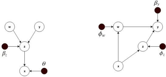
Fig. 4.1. Graphical models for the GMVAE showing the generative model (left) and the inference model (right).

The generative model shown in figure 4.1 provides a good intuition of what represents each variable. The idea is that the latent variableyrepresents the class of the data to be generated and the latent variable w captures variable attributes of the data. These two variables form the first latent hierarchical level. Finally, in the second latent hierarchical level is the variablez. This variable will have the form of a Gaussian mixture distribution

and it will be a representation of the multimodal nature of the data. Now that the intuitive meaning of each variable is clear, their definitions will make sense:

• Input data: x∼ p(x)

• Latent variable z: p(z)=∫ p(z|w,y)p(w)p(y)dwdy

• Latent variablew: p(w)= N(0,I)

• Latent variabley:y∼ Mult(π) given thatπi = _K1

4.3. Defining zdirectly as a GMM

The most direct solution to inject multi-modality into the latent space would be to use the standard VAE framework but definingzas a Gaussian mixture density.

p(z)= K ∑ i=1 ΠiN(µi,Σi) qϕ(z|x)= N(z|µϕ(x),Σϕ(x))

However, the problem with this approach is that using GMM makes the Kullback-Leibler divergence of the ELBOequation 3.8 intractable (see Appendix C). While it is possible to approximate it using Monte Carlo estimator, this increases the variance of the estimator. KL(qϕ(z|x)||p(z))= Ez∼qϕ [ logqϕ(z|x) p(z) ] ≈ 1 M M ∑ i=1 logqϕ(z (i)_|x) p(z(i)₎

Another problem with this approach is that it produces numerical instability during training when qϕ(z(i)|x) → 0 or p(z(i)) → 0 or both go to 0 (see section 5.6 for more information). Thus, this approach is discarded.

4.4. Optimization Function

As stated in the paper, the objective function (known as ELBO) is defined in the following manner:

ELBO=Eq[

pβz,θ(x,z,w,y)

qβy,ϕz,ϕw(z,w,y|x)

]

The definitions of pβz,θ(x,z,w,y) andqβy,ϕz,ϕw(z,w,y|x) can be arbitrarily chosen. For

From these definitions, it is important to remember that the parameters of each distribution means it is implemented using neural networks.

pβz,θ(x,z,w,y)= pθ(x|z)pβz(z|w,y)p(w)p(y) (4.1) qβy,ϕz,ϕw(z,w,y|x)= ∏ i pβy(y (i)_|w(i)_,z(i)_)q ϕz(z (i)_|x(i)_)q ϕw(w (i)_|x(i)_{) (4.2)}

The join density function pβz,θ(x,z,w,y) is decomposed in a multiplication of four

terms. The prior density functionsp(w) and p(y) are known (see section 4.3). The condi-tional distribution of z|w,yis defined as pβz(z|w,y) =

∏K

k=1N(µβz(w),Σβz(w))

[yk==1] _being

K the number of clusters selected a priori. Finally, the conditional distribution of x|zis defined as pθ(x|z)= N(µθ(z),Σ).

As it is done in the original paper, to simplify the notation only one data point at a time will be considered. Then, the conditional distributionqβy,ϕz,ϕw(z,w,y|x) is decomposed in

a multiplication of three terms. The conditional distributions of z|x and w|x are both defined as Gaussian beingqϕw(w|x) = N(µϕw(x),Σϕw(x)) andqϕz(z|x) = N(µϕz(x),Σϕz(x))

respectively. The distribution pβy(yj = 1|w

(i)_,z(i)_{) is parameterized byβ}

y because during

the experiments it will be modeled using a neural network to assure numerical stability (see section 5.6). However, the most accurate definition of such distribution is:

pβz(yj =1|w,z)=

p(yj =1)pβz(z|yj = 1,w)

∑K

k=1 p(yk =1)pβz(z|yk = 1,w)

Given this definition of the distributions and considering Eq ≡ Eqβy,ϕz,ϕw(z,w,y|x), the

ELBOfunction can be rewritten as:

ELBO= Eq [ p(w)p(y)pβz(z|w,y)pθ(x|z) qϕz(z|x)qϕw(w|x)pβz(y|w,z) ] = Eq[logpθ(x|z)]+Eq [ log pβz(z|w,y) qϕz(z|x) ] +Eq [ log p(w) qϕw(w|x) ] +Eq [ log p(y) pβ(y|w,z) ] = Eq[logpθ(x|z)]−Eq [ log qϕz(z|x) pβz(z|w,y) ] −Eq [ logqϕw(w|x) p(w) ] −Eq [ log pβz(y|w,z) p(y) ]

Each of the terms composing the ELBOhas a specific function. In order, they are named reconstruction term, conditional prior term, w-prior term and z-prior term. In the following sections each of these terms is operated and simplified as much as possible. The complete steps are shown in Appendix D.

4.4.1. Reconstruction Term

The first component is the reconstruction term. It measures the difference between the input data and their reconstruction. This term has exactly the same form as the first term of theELBO’s VAE.

Eq[logpθ(x|z)]≈

1

2σ2(x−µθ(z)) 2

4.4.2. Conditional prior term

The conditional prior term Eq [

log qϕz(z|x)

pβ(z|w,y)

]

measures the similarity between qϕz(z|x) and

pβ(z|w,y). As it is a positive value and appears with a negative sign in theELBOequation, the conditional prior term should be small in order to maximize the objective function. To be a small value, both probability functions should be similar to each other. Thus, this term is restricting the expressive capacity of the model: it is a regularizer.

In the model presented by Nat Dilokthanakul et al [6], this term is simplified and results in an expectation of a KL divergence. Then it is approximated using Monte Carlo.

Eqϕw(w|x)pβ(y|w,z) [ KL(qϕz(z|x)||pβ(z|w,y) )] ≈ 1 M M ∑ m=1 K ∑ k=1 pβ(yk =1|w(i),z(i))KL ( qϕz(z|x)||pβ(z|w (i)_, yk =1) )

To do the approximation, the latent variablewis sampled from qϕw(w|x) but it is not

clear howzis sampled to obtain the final result. For this reason, the simplified expression for this term has been derived in this thesis and it turns out it differs from the one proposed in the aforementioned paper.

Eq [ log qϕz(z|x) pβ(z|w,y) ] = Eqϕw(w|x)qϕz(z|x) ⎡ ⎢ ⎢ ⎢ ⎢ ⎢ ⎣ K ∑ k=1 ˜ πklog qϕz(z|x) pβ(z|w,yk =1) ⎤ ⎥ ⎥ ⎥ ⎥ ⎥ ⎦

As it can be observed, now it is clear this term can be approximated using the Monte Carlo estimator by samplingwfromqϕw(w|x) and zfromqϕz(z|x):

Eqϕw(w|x)qϕz(z|x) ⎡ ⎢ ⎢ ⎢ ⎢ ⎢ ⎣ K ∑ k=1 ˜ πklog qϕz(z|x) pβ(z|w,yk = 1) ⎤ ⎥ ⎥ ⎥ ⎥ ⎥ ⎦ ≈ 1 N 1 M N ∑ n=1 M ∑ m=1 K ∑ k=1 ˜ πklog qϕz(z (m)_|x) pβ(z(m)_|w(n),_y k =1)

This expression can be simplified considering only one sample for each variable.

Eqϕw(w|x)qϕz(z|x) ⎡ ⎢ ⎢ ⎢ ⎢ ⎢ ⎣ K ∑ k=1 ˜ πklog qϕz(z|x) pβ(z|w,yk = 1) ⎤ ⎥ ⎥ ⎥ ⎥ ⎥ ⎦ ≈ K ∑ k=1 ˜ πklog qϕz(z|x) pβ(z|w,yk =1)

Moreover, as all variables involved are distributed as Gaussians, it can be further sim-plified. For the complete details see Appendix D.

4.4.3. W-prior term

The w-prior termEq [

logqϕw(w|x)

p(w)

]

measures the similarity betweenqϕw(w|x) and p(w). As

it is a positive value and appears with a negative sign in theELBOequation, the w-prior term is also a regularizer. It can be written as a KL divergence of Gaussian distributions. Consequently, it can be computed analytically.

Eq [ logqϕw(w|x) p(w) ] = KL(qϕw(w|x)||p(w) ) Recalling that p(w)= N(0,I): KL(qϕw(w|x)||p(w) ) = 1 2 [ tr(Σϕw(x) ) −Dw−log det(Σϕw(x))+ ( µϕw(x) )T( µϕw(x) )] 4.4.4. Y-prior term

The y-prior termEq [

log pβ(_py₍|_yw₎,z)]measures the similarity between pβ(y|w,z) and p(y). As it is a positive value and appears with a negative sign in theELBOequation, the y-prior term is also a regularizer. It can be written as an expectation overqϕz(z|x) andqϕw(w|x) of

a KL divergence of categorical distributions.

Eq [ log pβ(y|w,z) p(y) ] =Eqϕz(z|x)qϕw(w|x) [ KL(pβ(y|w,z)||p(y))] KL(pβ(y|w,z)||p(y))= K ∑ i=1 p(yi =1) log p(yi =1) pβ(yi =1|w,z) Recalling that p(yi =1)= _K1 KL(pβ(y|w,z)||p(y))= −logK− 1 K K ∑ i=1 logpβ(yi = 1|w,z) 4.4.5. ELBO Equation

Joining the previous expressions, the lower bound function can be written as:

ELBO(ϕw, ϕz, β, θ)=Eqϕz(z|x)[logpθ(x|z)]−Eqϕw(w|x)qϕz(z|x) ⎡ ⎢ ⎢ ⎢ ⎢ ⎢ ⎣ K ∑ k=1 ˜ πklog qϕz(z|x) pβ(z|w,yk =1) ⎤ ⎥ ⎥ ⎥ ⎥ ⎥ ⎦− KL(qϕw(w|x)||p(w) ) −Eqϕz(z|x)qϕw(w|x) [ KL(pβ(y|w,z)||p(y) )] (4.3)

This is the expression that will be optimized during training, having applied reparam-eterization trick previously.

4.5. Reparameterization Trick

As it happens in the VAE, it is necessary to move the intermediate sampling layers to the input in order to be able to apply backpropagation. Therefore, the sampling fromqϕz(z|x)

andqϕw(w|x) is realized through two new input noises, ϵz ∼ N(0,I) and ϵw ∼ N(0,I), as

shown below: z=µϕz(x)+ϵ √ Σϕz(x)∼ qϕz(z|x)= N(z|µϕz(x),Σϕz(x)) w= µϕw(x)+ϵ √ Σϕw(x)∼qϕw(w|x)= N(w|µϕw(x),Σϕw(x))

In this way, backpropagation can be applied to optimize the network parameters since given a fixedx,ϵzandϵw, theELBOis deterministic and continuous, meaning it is possible

to use SGD to optimize it via backpropagation.

4.6. Sampling

The sampling of new data is straightforward. First,wandyare sampled from their corre-sponding prior distributions p(w)= N(0,I) and p(y)∼ Mult(π). Then zis sampled from

pβz(z|w,y) and injected into the decoder:

5. METHODOLOGY

This chapter presents everything related to the experiments conducted. It includes the objectives, the preparation of the data, the definition of the models’ architectures and hyperparameters, the problems found during training, the definitions of the metrics used to evaluate the results and finally some aspects related to the visualization of the results.

5.1. Objective

The purpose of the experiments conducted in this work is to understand the effect of diff er-ent configurations of the models’ hyperparameters and to assess if the GMVAE described in chapter 4 achieves superior performance, in terms of generative capability and latent space interpretability, compared to the standard VAE.

5.2. Prepare Data

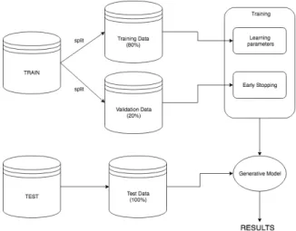
Both datasets used in this thesis are already cleaned and contain no missing data. They will be firstly split in test and train. Then the train set will be divided in two subsets as shown in Figure 5.1 to obtain a validation set. Thus, three subsets of images will be used to realize the experiments, each of them with a specific purpose:

• Training Data: data used in the learning process.

• Validation Data: data used to evaluate the loss in each epoch during training. It is not used in the learning process but to stop training earlier to prevent overfitting (stop training when validation error increases)

• Test Data: data used to generate results and assess the performance of the model.

5.3. Model Architecture

Three different types of neural networks have been used to build the models:

• DenseNet: Formed by simple fully connected layers.

• ConvNet: Formed by convolutional layers, pooling layers and a DenseNet at the end.

• DeconvNet: Formed by deconvolutional layers and a DenseNet at the beginning.

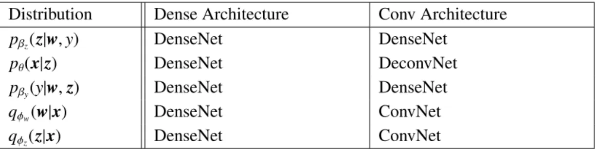
Then, with these three types of neural networks two types of architectures have been used to implement VAE and GMVAE. They have been namedDense Architecture and

Conv Architecture. Table 5.1 and Table 5.2 show how each distribution has been imple-mented for each architecture.

Distribution Dense Architecture Conv Architecture

qϕ(z|x) DenseNet ConvNet

pθ(x|z) DenseNet ConvNet

Table 5.1. VAE architectures

Distribution Dense Architecture Conv Architecture

pβz(z|w,y) DenseNet DenseNet

pθ(x|z) DenseNet DeconvNet

pβy(y|w,z) DenseNet DenseNet

qϕw(w|x) DenseNet ConvNet

qϕz(z|x) DenseNet ConvNet

Table 5.2. GMVAE architectures

5.4. Definition of hyperparameters

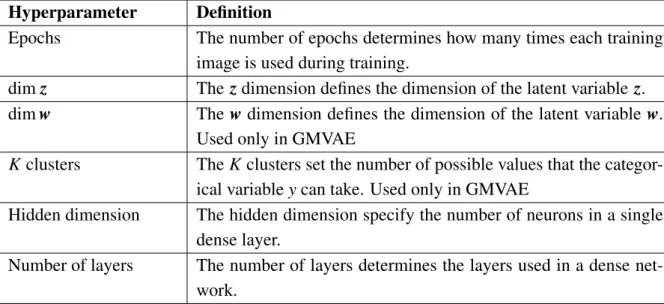
In general terms, when training a machine or deep learning algorithm there are a num-ber of parameters that can be selected before training. Some of them handle the files generated, others deal with saving and restoring a model and others determine certain as-pects of the algorithm. In order to test different configurations of the VAE and GMVAE algorithms, some parameters must variate. These are defined in Table 5.3.

Hyperparameter Definition

Epochs The number of epochs determines how many times each training

image is used during training.

dimz Thezdimension defines the dimension of the latent variablez.

dimw Thew dimension defines the dimension of the latent variablew.

Used only in GMVAE

Kclusters TheKclusters set the number of possible values that the categor-ical variableycan take. Used only in GMVAE

Hidden dimension The hidden dimension specify the number of neurons in a single dense layer.

Number of layers The number of layers determines the layers used in a dense net-work.

Table 5.3. Definition of hyperparameters.

5.5. Experimental Setup

To accomplish the goals defined previously, the following experiments were conducted:

• Experiment 1. Train VAE using different configuration of the hyperparamters (shown in Table 5.4). Evaluate the results using the metrics defined in Section 5.8. Com-pare the latent space representation and input’s reconstruction with the results PCA achieves.

• Experiment 2. Train GMVAE changing dimw (see Table 5.5) to understand the information learnt by the latent variables wand z. Evaluate the results in terms of interpretability.

• Experiment 3. Train GMVAE using the best configurations obtained in experiment 1 in terms of generative and reconstruction capabilities. As the dataset consists of handwritten numbers from 0 to 9, it is known the number of classes is 10, therefore

K =10. Evaluate the results using the metrics defined in Section 5.8.

• Experiment 4. Evaluate the log likelihood of VAE and GMVAE models trained in previous experiments when uniform and dropout noise is added to the input. The uniform noise (soft) adds±0.1 to each normalized pixel and the dropout noise (strong) sets to 0 half of the pixels.

• Experiment 5. Train GMVAE and VAE using convolutional and deconvolutional networks. Compare the results with respect to the ones obtained in experiment 3 and experiment 1. Evaluate performance using "Frey faces" dataset. Configuration is shown in Table 5.6.

All models have been trained using images as input. As it is known, the most efficient way to deal with images is to use convolutional layers. However, simple fully connected dense networks have been used for the first four experiments in order to minimize training time.

The selection of the set of values for each hyperparameter was based on hyperparam-eters selected in similar works and on interpretability.

Experiment 1

Generative model VAE

Model name model1

Dataset MNIST

Architecture Dense Architecture

σ2 _{[0.01, 0.001]}

dimz [2, 10, 20, 50]

Hidden layers [2, 3, 4]

Hidden dimension [64, 128]

Table 5.4. Experiment 1 Hyper-Parameters.

Experiment 2

Generative model GMVAE

Model name model4_bias

Dataset MNIST

Architecture Dense Architecture

σ2 _0.001 dimz 10 dimw [2, 10, 20] K 10 Hidden layers 3 Hidden dimension 128

Experiment 5

Generative model [GMVAE, VAE]

Model name [model5, model2]

Dataset [MNIST, FREY]

Architecture Conv Architecture

Table 5.6. Experiment 5 Hyper-Parameters.

Next section describes some problems encountered during training.

5.6. GMAVE numerical stability

In the first attempt to implement the GMVAE, numerical stability problems were found. At some point during training (usually at the beginning), NaN values appeared in the loss function. As a consequence, training stopped.

After a sound analysis, it was found the numerical instability was originated in the evaluation of the distribution pβ(yj = 1|w,z):

pβ(yj = 1|w,z)= p(yj =1)pβ(z|yj = 1,w) ∑K k=1p(yk =1)pβ(z|yk = 1,w) = π˜jN(z|µβ(w) yj, σ2 β(w)yj) ∑K k=1π˜kN(z|µβ(w)yk, σ2_β(w)yk)

The problem arose when evaluating z in pβ(z|yj = 1,w), which is assumed to be a

Gaussian distribution. If z is at great distance from the mean of the distribution, the probability is approximately 0. On the other hand, if the variance learnt tends to 0 or ∞ problems arise. In these cases, the evaluation of the probabilities pβ(z|yk = 1,w) or

pβ(yj = 1|w,z) may be of indeterminate form, for example 0₀ or 0x∞, which causes the

program to throw aNaN value.

In order to solve this problem and reach a robust implementation, three complemen-tary solutions have been approached:

• Change the definition of pβ(yj =1|w,z)

• Restrict the output of the neural networks related to variables zandw. • Reduce the learning rate

5.6.1. Approximation ofpβ(yj =1|w,z)

As described previously, the direct evaluation ofpβ(yj = 1|w,z) leads to numerical

Softmax approximation

The first idea was to approximate pβ(yj = 1|w,z) with a softmax function.

Neverthe-less, it also had numerical stability issues.

vj = z−µβ(w) yj pβ(yj = 1|w,z)= so f tmax(vj)= evj ∑K k=1evk

As explained in the next section, the problem was mitigated by limiting the range values of several neural networks outputs. However, the limitations were so strong that the model performed poorly. This alternative was discarded.

Constant PDF

The next alternative was to simplify the model by definingpβ(yj =1|w,z) as :

pβ(yj =1|w,z)=

1

K∀j

This way, it is not required to evaluate the probabilities pβ(z|yk = 1,w) so, obviously,

the instability problem disappears. However this is a strong assumption that reduces the expressivity of the model. Thus, further alternatives were sought.

Neural network approximation

The final approach was to approximate the PDF using a neural network composed of fully connected layers. The input of this neural network is the concatenation ofwand z

and the output is the probability for eachyj.:

pβ(yj = 1|w,z)=qβy(yj =1|[w,z])

This resulted in a robust training as the numerical instability problem disappeared: there is no need to evaluate pβ(z|yk = 1,w). Moreover, the dependency of yon zandw

still remains and the y-prior term of theELBOprevents overfitting on this neural network.

5.6.2. Output restrictions

As described above, the instability problem arise when the variablezmust be evaluated at distant points from the mean of the distribution or its variance tends to 0 or∞. However this situation is nonsense as every image should have a latent representation that is related to one cluster and extreme values of the parameters of the Gaussian distributions are not interpretable. This is the reason to impose constrains in the PDFs pβz(z|w,y) andqϕz(z|x).

In other words, to impose restrictions in the output range of the following neural networks:

• µ_ϕz(x),µβz(w)

• σ2

ϕz(x),σ

2

βz(w)

yj

To restrict the possible values of outputs of the neural networks modeling the means and the variances it has been used ϕ(x) = A∗ t f.tanh(x), where A ∈ [1,100], as the activation function of the last layer of the neural networks. Moreover, as the variance cannot be negative neither close to zero, the following sigma function was defined, being

xthe output of the neural network:

σ2_(x)=ex_{→ σ}2_{(x)= log (e}x₊

1)+0.1=t f.so f t plus(x)+0.1

With this definition of the variance and the constrains in the range of outputs the problem is solved.

5.7. Motivate clustering behaviour

Other problem found is anti-clustering behaviour. As it is stated in [6], thez-prior term can degenerate the clustering nature of the latent variablez. It is a regularization term that may go to 0 if all the clusters merge into a single one. This over-regularization issue is an open problem under research.

To stimulate clustering behaviour, the bias for the last layer of the neural networks

µϕz(x) andµβz(w)

yj _{is not initialize with zeros (as usual) but as a truncated normal. We are}

just providing the model with a priori knowledge to facility the learning process.

5.8. Metrics

The selection of metrics to evaluate the performance of generative models is still an open discussion in spite of the fact that there has been significance progress. In general terms, a good metric should:

• Measure the visual interpretation of samples (subjective). • Maximize the log-likelihood.

It would be perfect to have a measurement of how realistic a human perceive a gen-erated image and just maximize it. However, this is hard to quantify and it is still under research. Alternately there are different metrics such as visual fidelity of samples, log-likelihood, Parzen window estimates or Inception Score [35].

As it is shown in [36], the metrics to evaluate a generative model must be chosen in accordance with the objectives of the application. There is not an universal criterion that fits perfectly for all applications and goals of generative models. Furthermore, good performance with respect to one criterion does not necessarily imply good performance

in other metrics. For example, high log-likelihood does not guarantee realistic generated data [36]. Therefore, it is important to examine the goal when selecting the evaluation technique.

For this thesis, the goal is to assess generative models in terms of image synthesis and latent variable interpretability. As such, table 5.7 shows the metrics selected.

Quantitative Metrics Qualitative Metrics

ELBO Quality of generated images

Average log-likelihood Latent space interpretability

Table 5.7. Metrics selected.

The ELBO function differs slightly between VAE (see Equation 3.8) and GMVAE (see Equation 4.3). It is the function maximized during training.

The average log-likelihood E[logp(x|z)] measures the reconstruction capabilities of the model (it is not related to the generative capacity). It is the same for all models and has the following form.

E[logp(x|z)]≈ 1 N N ∑ i=1 1 K K ∑ k=1 logp(x(i)|z(_ki)) logp(x(i)|z_k(i))= −Dx 2 log(2πσ 2₎₋ 1 2σ2(x (i)_−µ(z(i) k )) 2

Notice it is calculated sampling severalzfor each datum in the dataset to reach a better approximation.

The latent space interpretability will be appraised visually in terms of how well the multimodal nature of the data is represented in the latent space.

The quality of the generated images will be assessed through human visual inter-pretation. However, to simplify this task, only the models’ configurations with smaller

KL(q(z|x)||p(z)) will be chosen in advance. Recall that a smallKL(∗) means the distribu-tion of the data in the latent space is close to the distribudistribu-tion from which generated data will be sampled.

5.9. Visualization of results

A very important aspect in deep learning is the visualization of the results. In this study the results are the generated/reconstructed images and the distribution of the latent vari-ables. The visualization of the images is straightforward. However, the latent variables

sometimes are high dimensional so it is impossible to understand them in their raw di-mension. Therefore, they are represented in 2D or 3D plots through a dimensionality reduction algorithm such as PCA or t-SNE.

6. RESULTS

This chapter analyzes the results obtained from the implementation of the previously described models. The source code is available at GitHub through the following URL:

https://github.com/psanch21/VAE-GMVAE.

6.1. Initial considerations

This chapter contains several tables that show the value of the loss function (the nega-tiveELBOfunction) at the end of the training process. These tables contain at least two columns calledValidLossandTrainingLossthat refer to the negative ELBOfunction for the validation and train dataset respectively. These tables may contain other columns that represent the terms composing the ELBO function. Moreover, these tables contains a column calledModelNamethat holds information about the model configuration. For the case of VAE models (model1 or model2) this column has the following format{model Type}_{dataset Name}_{epochs}_{sigma Recons}_{dimZ}_{dimHidden}_{num Layers}

and for the case of GMVAE models (model4_bias or model5) it has this format{model Type}_{dataset Name}_{epochs}_{sigma Recons}_{dim Z}_{dim W}_{dim Hidden}_{num Layers}_{K clusters}.

Another important consideration is that the range of the reconstruction loss and there-fore the total loss depends on the chosen value forσ2_{. So it is important to keep this in}

mind when comparing different configurations.

6.2. Experiment 1: VAE

Results for the different configurations of the VAE model show that it presents enormous difficulties to achieve good clustering and generation results at the same time. Tables 6.1 and 6.2 show the final loss of the configurations that resulted in the best clustering and generation capabilities respectively. The entire table with the results for all the configura-tions tested is included in Appendix A. Furthermore, Appendix B includes some examples of poorly generated samples.

Table 6.1. Loss results of the best clustering configurations. Ordered by ValidLoss.

Table 6.2. Loss results of the best generative configurations. Ordered by KLloss.

Analyzing the tables it is import to remark that the value of the KL and the dimension of the latent variable determine how the model behaves. Configurations that produce good clustering present larger dimension on the latent variable (dimz = 10) and large KL (around 35−55). On the other hand, configurations that obtain good generation are those with smaller dimension of the latent variable (dimz = 2) and smaller KL (around 13−40).

Figures 6.1 and 6.2 show examples of good clustering and good generation results respectively. In the first case, the multimodal nature is captured clearly but the generated samples are terrible, just a few of them can be considered realistic. The second case generates a lot of realistic samples (although a bit fuzzy). However, only the images representing the number 1 are visibly separated in the latent space, the others are mixed together.

(a)Generated images (b)Latent space (c)Reconstruction Fig. 6.1. Example of good clustering but poor generation result.