Asset Float and Speculative Bubbles
Harrison Hong, Jos´
e Scheinkman, and Wei Xiong
∗Princeton University
April 19, 2004
Abstract
We model the relationship between float (the tradeable shares of an asset) and stock price bubbles. Investors trade a stock that initially has a limited float because of insider lock-up restrictions but the tradeable shares of which increase over time as these restrictions expire. A speculative bubble arises because investors, with heterogeneous beliefs due to overconfidence and facing short-sales constraints, anticipate the option to resell the stock to buyers with even higher valuations. With limited risk absorption capacity, this resale option depends on float as investors anticipate the change in asset supply over time and speculate over the degree of insider selling. Our model yields implications consistent with the behavior of internet stock prices during the late nineties, such as the bubble, share turnover and volatility decreasing with float and stock prices tending to drop on the lock-up expiration date though it is known to all in advance.
∗
We thank the National Science Foundation for financial support. We also thank Lasse Pedersen, Jeremy Stein and Dimitri Vayanos and seminar participants at the DePaul University-Chicago Federal Reserve, Duke University, NBER Asset Pricing Meeting, SEC, University of Iowa, and Wharton School for their comments. Please address inquiries to Wei Xiong, 26 Prospect Avenue, Princeton, NJ 08540, [email protected].
1
Introduction
The behavior of internet stock prices during the late nineties was extraordinary. On Febru-ary of 2000, this largely profitless sector of roughly four-hundred companies commanded valuations that represented six percent of the market capitalization and accounted for an astounding 20% of the publicly traded volume of the U.S. stock market (see, e.g., Ofek and Richardson (2003)).1 These figures led many to believe that this set of stocks was in the midst of an asset price bubble. These companies’ valuations began to collapse shortly thereafter and by the end of the same year, they had returned to pre-1998 levels, losing nearly 70% from the peak. Trading volume and return volatility in these stocks also largely dried up in the process.
Many point out that the collapse of internet stock prices coincided with a dramatic ex-pansion in the publicly tradeable shares (or float) of internet companies (see, e.g., Cochrane (2003)). Since many internet companies were recent initial public offerings (IPO), they typically had 80% of their shares locked up—the shares held by insiders and other pre-IPO equity holders are not tradeable for at least six months after the IPO date.2 Ofek and Richardson (2003) document that at around the time when internet valuations collapsed, the float of the internet sector dramatically increased as the lock-ups of many of these stocks expired.3 Despite such tantalizing stylized facts, there has been little formal analysis of this issue.
In this paper, we attempt to understand the relationship between float and stock price bubbles. Our analysis builds on early work regarding the formation of speculative bubbles due to the combined effects of heterogeneous beliefs (i.e. agents agreeing to disagree) and
1The average price-to-earnings ratio of these companies hovered around 856. And the relative valuations of
equity carveouts like Palm/3Com suggested that internet valuations were detached from fundamental value (see, e.g., Lamont and Thaler (2003), Mitchell, Pulvino, and Stafford (2002)).
2In recent years, it has become standard for some 80% of the shares of IPOs to be locked up for about six months.
Economic rationales for lock-ups include a commitment device to alleviate moral hazard problems, to signal firm quality, or rent extraction by underwriters.
3
They find that, from the beginning of November 1999 to the end of April 2000, the value of unlocked shares in the internet sector rose from 70 billion dollars to over 270 billion dollars.
short-sales constraints (see, e.g., Miller (1977), Harrison and Kreps (1978), Chen, Hong and Stein (2002) and Scheinkman and Xiong (2003)). In particular, we follow Scheinkman and Xiong (2003) in assuming that overconfidence—the belief of an agent that his information is more accurate than what it is—is the source of disagreement. Although there are many dif-ferent ways to generate heterogeneous beliefs, a large literature in psychology indicates that overconfidence is a pervasive aspect of human behavior. In addition, the assumption that investors face short-sales constraints is also eminently plausible since even most institutional investors such as mutual funds do not short.4
More specifically, we consider a discrete-time, multi-period model in which investors trade a stock that initially has a limited float because of lock-up restrictions but the trade-able shares of which increase over time as insiders become free to sell their positions. We assume that there is limited risk absorption capacity (i.e. downward sloping demand curve) for the stock.5 Insiders and investors observe the same publicly available signals about fun-damentals. In deciding how much to sell on the lock-up expiration date, insiders process the same signals with the correct prior belief about the precision of these signals. How-ever, investors are divided into two groups and differ in their interpretation of these signals. Since each group overestimates the informativeness of a different signal, they have distinct forecasts of future payoffs. As information flows into the market, their forecasts change and the group that is relatively more optimistic at one point in time may become at a later date relatively more pessimistic. These fluctuations in expectations generate trade. Importantly, investors anticipate changes in asset supply over time due to potential insider selling.
When investors have heterogeneous beliefs due to overconfidence and are short-sales
4Roughly 70% of mutual funds explicitly state (in Form N-SAR that they file with the SEC) that they are not
permitted to sell short (see Almazan, Brown, Carlson and Chapman (1999)). Seventy-nine percent of equity mutual funds make no use of derivatives whatsoever (either futures or options), suggesting that funds are also not finding synthetic ways to take short positions (see Koski and Pontiff (1999)). These figures indicate the vast majority of funds never take short positions.
5
It is best to think of the stock as the internet sector. This assumption is meant to capture the fact that many of those who traded internet stocks were individuals with undiversified positions and that there are other frictions which limit arbitrage. For instance, Ofek and Richardson (2003) report that the median holding of institutional investors in internet stocks was 25.9% compared to 40.2% for non-internet stocks. For internet IPO’s, the comparable numbers are 7.4% to 15.1%. See Shleifer and Vishny (1997) for a description for various limits of arbitrage.
constrained, they pay prices that exceed their own valuation of future dividends as they anticipate finding a buyer willing to pay even more in the future. The price of an asset exceeds fundamental value by the value of this resale option; as a result, there is a bubble component in asset prices.6 When there is limited risk absorption capacity, the two groups naturally want to share the risk of holding the supply of the asset. Hence they are unwilling to hold all of the tradeable shares without a substantial risk discount.
A larger float or a lower risk absorption capacity means that it takes a greater divergence in opinion in the future for an asset buyer to resell the shares, which means the less valuable the resale option is today. So, ex ante, agents are less willing to pay a price above their assessments of fundamentals and the smaller is the bubble. Indeed, we show that the strike price of the resale option depends on the relative magnitudes of asset float to risk absorption capacity—the greater is this ratio, the higher the strike price for the resale option to be in the money.
Since the demand curve for the stock is downward sloping, price naturally declines with supply even in the absence of speculative trading. But when there is speculative trading, price becomes even more sensitive to asset float—i.e. overconfidence leads to a multiplier effect. This multiplier effect is highly nonlinear—it is much bigger when the ratio of float to risk bearing capacity is small than when it is large. Furthermore, since trading volume and share return volatility are tied to the amount of speculative trading, these two quantities also decrease with the ratio of asset float to risk absorption capacity. As a result, our model predicts that a decrease in price associated with greater asset supply is accompanied by lower turnover and return volatility. These auxiliary effects related to turnover and volatility are absent from standard models of asset pricing with downward sloping demand curves.
Perhaps the most novel feature of our model has to do with speculation by investors about the trading positions of insiders after lock-ups expire. Since investors are overconfident, each group thinks that they are smarter than the other group. A natural question that
6
arises is how they view insiders and how insiders process information about fundamentals. Since insiders are typically thought of as having more knowledge about their company than outsiders, it seems natural to assume that each group of investors thinks that the insiders are “smart” like them (i.e. sharing their expectations as opposed to the other group’s). Indeed, we assume that they agree to disagree about this proposition.
As a result, each group of investors expects the other group to be more aggressive in taking positions in the future when the other group has a higher valuation. The reason is that the other group expects that the insiders will eventually come in and share the risk of their positions with them. Since agents are more aggressive in taking on speculative positions, the resale option and hence the bubble is larger. Just as long as insiders are not infinitely risk averse and they decide how to sell their positions based on their belief about fundamentals, this effect will be present. In other words, the very event of potential insider selling at the end of the lock-up period leads to a larger bubble than would have otherwise occurred.
Using these results, it is easy to see that our theory yields a number of predictions that are consistent with stylized facts regarding the behavior of internet stocks during the late nineties. One of the most striking of these stylized facts is that the internet bubble bursted in the Winter of 2000 when the float of the internet sector dramatically increased. Moreover, trading volume and return volatility also dried up in the process.
Our model can rationalize these stylized facts for a couple of reasons. While internet stocks had different lock-up expiration dates, the empirical findings suggest that a substan-tial fraction of these stocks had lock-ups that expired at around the same time. Taking the stock in our model to be the internet sector, a key determinant of the size of the bubble is the ratio of the float to risk absorption capacity in this sector. To the extent that the risk ab-sorption capacity in the internet sector stayed the same but the asset supply increased, our model predicts that it requires a bigger divergence of opinion to sustain the bubble, leading to a smaller bubble and less trading volume and volatility. Moreover, after the expiration
of lock-up restrictions, speculation regarding the degree of insider selling also diminished, again leading to a smaller internet bubble. We show that the drop in prices related to an increase in float can be dramatic and is related to the magnitude of the divergence of opinion among investors.
There are of course a number of other plausible reasons for why the collapse of the internet bubble coincided with the expansion of float in the sector. The two most articulated is that short-sales constraints became more relaxed with the expansion of float and that investors learned after lock-ups expired that the companies may not have been as valuable as they once thought. Our model provides a compelling and distinct third alternative. For instance, a bubble bursts with an expansion of asset supply in our model without any change in the cost of selling. We think this is one of the virtues of this model, for while short-selling costs are lower for stocks with higher float, empirical evidence indicates that it is difficult to tie the decline in internet valuations in the Winter of 2000 merely to a relaxation of short-sales constraints.7 Moreover, neither a relaxation of short-sales-constraints story nor a representative-agent learning story can easily explain why trading volume and return volatility also dried up after the bubble bursted.
Another outstanding stylized fact regarding internet stocks during the late nineties in-volve price dynamics across the lock-up expiration date. Empirical evidence suggests that on this date, stock prices tend to decline though the day of the event is known to all in advance.8 Our model is able to rationalize this finding. Since investors are overconfident and incorrectly believe that the insiders share their beliefs, to the extent that the insiders’ belief is rational (i.e. properly weighing the two public signals) and some investors are more optimistic than insiders, there will be more selling on the part of insiders on the date of lock-up expiration than is anticipated by outside investors. Hence, the stock price tends to fall on this date.
7
See Ofek and Richardson (2003). Indeed, it is difficult to account for differences, at a given point in time, in the valuations of the internet sector and their non-internet counterpart to differences in the cost-of-short-selling alone.
8
Finally, our model has implications for the cross-section of expected returns. One of the main testable implications is that even controlling for asset supply and risk bearing capacity, a stock in which there is the potential for insider selling will have a larger bubble. Presumably stocks with little float to begin with are the ones that are the most likely to have this potential. Therefore, our model predicts that in the cross-section, stocks with less float, even controlling for firm size, will have a larger speculative bubble component and hence a lower expected return.
Our paper proceeds as follows. In Section 2, we review related literature and highlight some of the contributions of our model. A simple version of the model without insider selling is described in Section 3. We present the solution for the general model with insider selling and time varying float in Section 4. We provide further discussions in Section 5 and conclude in Section 6. All proofs and some numerical examples are in the Appendix.
2
Related Literature
There is a large literature on the effects of heterogeneous beliefs on asset prices and trading volume. Miller (1977) and Chen, Hong and Stein (2002) analyze the overvaluation generated by heterogeneous beliefs and short-sales constraints. These models are static and hence cannot generate an option value related to the dynamics of trading as in our model. Harris and Raviv (1993), Kandel and Pearson (1995), and Kyle and Lin (2002) study models where trading is generated by heterogeneous beliefs. Hong and Stein (2003) consider a model in which heterogeneous beliefs and short-sales constraints lead to market crashes. Harrison and Kreps (1978), Morris (1996) and Scheinkman and Xiong (2003) develop models in which there is a speculative component to asset prices. However, the agents in these last three models are risk-neutral, and so float has no effect on prices.
There are a number of ways to generate heterogeneous beliefs. One tractable way is to assume that agents are overconfident, i.e. they overestimate the precision of their knowledge in a number of circumstances, especially for challenging judgment tasks. Many studies from
psychology find that people indeed exhibit overconfidence (see Alpert and Raiffa (1982) or Lichtenstein, Fischhoff, and Phillips (1982)). In fact, even experts can display overconfi-dence (see Camerer (1995)). A phenomenon related to overconfioverconfi-dence is the “illusion of knowledge”—people who do not agree become more polarized when given arguments that serve both sides (see Lord, Ross and Lepper (1979)).9
Motivated by this research in psychology, researchers in finance have developed models to analyze the implications of overconfidence on financial markets (see, e.g., Kyle and Wang (1997), Odean (1998), Daniel, Hirshleifer and Subrahmanyam (1998) and Bernardo and Welch (2001).) In these finance papers, overconfidence is typically modelled as overestima-tion of the precision of one’s informaoverestima-tion. We follow a similar approach, but highlight the speculative motive generated by overconfidence.
The bubble in our model, based on the recursive expectations of traders to take advantage of mistakes by others, is different from “rational bubbles”.10 In contrast to our set up, rational-bubble models are incapable of connecting bubbles with asset float. In addition, in these models, assets must have (potentially) infinite maturity to generate bubbles.
Other mechanisms have been proposed to generate asset price bubbles (see, e.g., Allen and Gorton (1993), Allen, Morris, and Postlewaite (1993), Duffie, Garleanu and Pedersen (2002) ). But only one of these, Duffie, Garleanu and Pedersen (2002), has some implications for the relationship between float and asset price bubbles. They provide a dynamic model to show that the security lending fees that a stock holder expects to collect contribute an extra component to current stock prices, and that this component also decreases with asset float. In other words, an increase in float leads to lower lending fees (lower shorting costs) and hence lower prices.
As we mentioned earlier, our mechanism holds even if shorting costs are fixed and hence is distinct from that of Duffie, Garleanu and Pedersen (2002). Moreover, the empirical evidence indicates only minor reductions in the lending fee on average after lockup expirations during
9
See Hirshleifer (2001) and Barber and Odean (2002) for reviews of this literature.
the internet bubble, suggesting a need for alternative mechanisms such as ours to explain the relationship between float and asset prices during this period.
3
A Simple Model without Insider Selling
We begin by providing a simple version of our model without any insider selling. This special case helps develop the intuition for how the relative magnitudes of the supply of tradeable shares and investors’ risk-absorption capacity affect a speculative bubble. Below, this version is extended to allow for time-varying float due to the expiration of insider lock-up restrictions.
We consider a single traded asset, which might represent a stock, a portfolio of stocks such as the internet sector, or the market as a whole. There are three dates,t = 0,1,2. The asset pays off ˜f att = 2, where ˜f is normally distributed. A total of Q shares of the asset are outstanding. For simplicity, the interest rate is set to zero.
Two groups of investors, A and B, trade the asset at t = 0 and t = 1. Investors within each group are identical. They maximize a per-period objective of the following form:
E[W]− 1
2ηV ar[W], (1)
whereη is the risk-bearing capacity of each group. In order to obtain closed-form solutions, we need to use these (myopic) preferences so as to abstract away from dynamic hedging considerations. While unappetizing, it will become clear from our analysis that our results are unlikely to change qualitatively when we admit dynamic hedging possibilities. We further assume that there is limited risk absorption capacity in the stock.11
At t = 0, the two groups of investors have the same prior about ˜f, which is normally distributed, denoted by N( ˆf0, τ0), where ˆf0 and τ0 are the mean and precision of the belief, respectively. At t= 1, they receive two public signals:
sAf = ˜f +Af, sBf = ˜f +Bf, (2)
11
In other words, the asset demand curve is downward sloping. This is meant to simultaneously capture the undiversified positions of individual investors and frictions that limits arbitrage among institutional investors.
where Af and Bf are noises in the signals. The noises are independent and normally dis-tributed, denoted by N(0, τ), where τ is the precision of the two signals. Due to
over-confidence, group A over-estimates the precision of signal A as φτ, where φ is a constant
parameter larger than one. In contrast, group B over-estimates the precision of signal B as
φτ.
We first solve for the beliefs of the two groups at t = 1. Using standard Bayesian updating formulas, they are easily characterized in the following lemma.
Lemma 1 The beliefs of the two groups of investors at t = 1 are normally distributed, denoted by N( ˆf1A, τ) and N( ˆf1B, τ), where the precision is given by
τ =τ0+ (1 +φ)τ, (3)
and the means are given by ˆ f1A= ˆf0+ φτ τ (s A f −fˆ0) + τ τ (s B f −fˆ0), (4) ˆ f1B= ˆf0+ τ τ (s A f −fˆ0) + φτ τ (s B f −fˆ0). (5)
Even though the investors share the same prior about the terminal asset payoff and receive the same two public signals, the assumption that they place too much weight on different signals leads to a divergence in their beliefs. Their expectations converge in the limit as φ
approaches one.
Given the forecasts in Lemma 1, we proceed to solve for the equilibrium holdings and price at t = 1. With mean-variance preferences and short-sales constraints, it is easy to show that, given the price p1, the demands of investors (xA1, xB1) for the asset are given by
xA1 = max[ητ( ˆf1A−p1),0], xB1 = max[ητ( ˆf
B
1 −p1),0]. (6) Consider the demand of the group A investors. Since they have mean-variance preferences, their demand for the asset without short-sales constraints is simplyητ( ˆf1A−p1). When their beliefs are less than the market price, they would ideally want to short the asset. Since they
cannot, they simply sit out of the market and submit a demand of zero. The intuition for B’s demand is similar.
Imposing the market clearing condition, xA
1 +xB1 =Q, gives us the following lemma:
Lemma 2 Let l1 = ˆf1A−fˆ1B be the difference in opinion between the investors in groups A and B at t= 1. The solution for the stock holdings and price on this date are given by the following three cases:
• Case 1: If l1 > ητQ, xA1 =Q, xB1 = 0, p1 = ˆf1A− Q ητ. (7) • Case 2: If |l1| ≤ ητQ, xA1 =ητ l1 2 + Q 2ητ ! , xB1 =ητ −l1 2 + Q 2ητ ! , p1 = ˆ f1A+ ˆf1B 2 − Q 2ητ. (8) • Case 3: If l1 <−ητQ, xA1 = 0, xB1 =Q, p1 = ˆf1B− Q ητ. (9)
Since the investors are risk-averse, they naturally want to share the risks of holding the
Q shares of the asset. So, unless their opinions are dramatically different, both groups of investors will be long the asset. This is the situation described in Case 2. In this case, the asset price is determined by the average belief of the two groups, and the risk premium 2Qητ is determined by the total risk-bearing capacity. When group A’s valuation is significantly greater than that of B’s (as in Case 1), investors in group A hold allQshares, and those in B sit out of the market. As a result, the asset price is determined purely by group A’s opinion,
ˆ
f1A, adjusted for a risk discount, ητQ, reflecting the fact that this one group is bearing all the risks of the Q shares. The situation in Case 3 is symmetric to that of Case 1 except that group B’s valuation is greater than that of A’s.
We next solve for the equilibrium at t = 0. Given investors’ mean-variance preferences, the demand of the agents at t= 0 are given by
xA0 = max " η(EA0p1−p0) ΣA ,0 # , xB0 = max " η(EB0p1−p0) ΣB ,0 # , (10)
where ΣA and ΣB are the next-period price change variances under group-A and group-B investors’ beliefs:
ΣA =V arA0[p1−p0], ΣB =V arB0[p1−p0]. (11) Since investors in group A and group B have the same prior, ΣA equals ΣB. We denote them as Σ. (Moreover, note that EA
0[p1] = EB0[p1] as well.) It then follows that when we impose the market clearing condition at t= 0, xA
0 +xB0 =Q, the equilibrium price att = 0 is p0 = 1 2(E A 0[p1] + EB0[p1])− Σ 2ηQ. (12)
The key to understanding this price is to evaluate the expectation of p1 att = 0 under either of the investors’ beliefs (since they will also be the same, we will calculate EB0[p1] without loss of generality). To do this, it is helpful to re-write the equilibrium price from Lemma 2 (equations (7)-(9)) in the following form:
p1 = ˆf1B− Q 2ητ + −2Qητ if l1 <−ητQ 1 2l1 if − Q ητ < l1 < Q ητ l1 −2Qητ if ητQ < l1 , (13)
where l1 = ˆf1A−fˆ1B. From Lemma 1, it is easy to show that
l1 = (φ−1)τ τ ( A f − B f). (14)
So l1 has a Gaussian distribution with a mean of zero and a variance of
σl2 = (φ−1)
2(φ+ 1)τ
φ[τ0 + (1 +φ)τ]2
l
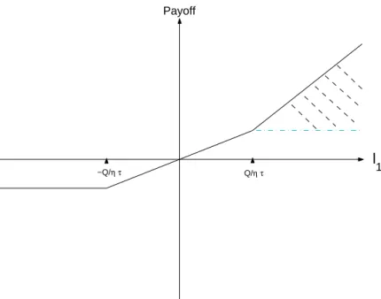
1 Payoff
−Q/ητ Q/ητ
Figure 1: The payoff from the resale option
under the beliefs of either group B (or A) agents.
For the expectation of B-investors at t = 0, there are two uncertain terms in equation (13), ˆf1B and a piecewise linear function of the difference in beliefs l1. This piecewise linear function has three linear segments, as shown by the solid line in Figure 1. The expectation of ˆf1B at t = 0 is simply ˆf0. This is simply the investors’ valuation for the asset if they were not allowed to sell their shares at t= 1. The three-piece function represents the value from being able to trade at t = 1. Calculating its expectation amounts to integrating the area between the solid line and the horizontal axis in Figure 1 (weighting by the probability density of l1). Since the difference in beliefs l1 has a symmetric distribution around zero, this expectation is simply determined by the shaded area, which is positive.
Intuitively, with differences of opinion and short-sales constraints, the possibility of sell-ing shares when other investors have higher beliefs provides a resale option to the asset owners (see Harrison and Kreps (1978) and Scheinkman and Xiong (2003)). If φ = 1, the possibility does not exist. Otherwise, the payoff from the resale option depends on the potential deviation of A-investors’ belief from that of B-investors. Following the same logic,
we can also derive a similar resale option value for A-investors.
The following theorem summarizes the expectation of A- and B-investors at t = 0 and the resulting asset price.
Theorem 1 At t= 0, the conditional expectation of A-investors and B-investors regarding
p1 are identical: EA0[p1] = EB0[p1] = ˆf0− Q 2ητ + E " l1− Q ητ ! I{l 1>ητQ} # , (16)
and the price at time 0 is
p0 = ˆf0− Σ 2ηQ− Q 2ητ + E " l1− Q ητ ! I{l 1>ητQ} # . (17)
There are four parts in the price. The first part, ˆf0, is the expected value of the funda-mental of the asset. The second term, 2ΣηQ, equals the risk premium for holding the asset from t= 0 to t= 1. The third part, 2Qητ, represents the risk premium for holding the asset from t= 1 to t= 2. The last term
B(Q/η) = E " l1− Q ητ ! I{l 1>ητQ} # (18) = √σl 2πe − Q2 2η2τ2σ2 l − Q ητN − Q ητ σl ! (19) represents the option value from selling the asset to investors in the other group when they have higher beliefs (the shaded area shown in Figure 1). Its format is similar to a call option with a strike price of ητQ. Therefore, an increase in Q or a decrease in η would raise the strike price of the resale option, and will reduce the option value.
More formally, we show in the following proposition:
Proposition 1 The size of the bubble decreases with the relative magnitudes of supply Q
to risk absorption capacity η, and increases with the overconfidence parameter φ.
Intuitively, when agents are risk averse, the two groups naturally want to share the risk of holding the shares of the asset. Hence they are unwilling to hold the float without a
substantial price discount. A larger float means that it takes a greater divergence in opinion in the future for an asset buyer to resell the shares, which means a less valuable resale option today. So, ex ante, agents are less willing to pay a price above their assessments of fundamentals and the smaller is the bubble.
Since there is limited risk absorption capacity, price naturally declines with supply even in the absence of speculative trading. But when there is speculative trading, price becomes even more sensitive to asset supply—i.e. a multiplier effect arises. To see this, consider two firms with the same share price, except that one’s price is determined entirely by fundamentals whereas the other includes a speculative bubble component as described above. The firm with a bubble component has a smaller fundamental value than the firm without to give them the same share price. We show that the elasticity of price to supply for the firm with a speculative bubble is greater than that of the otherwise comparable firm without a bubble. This multiplier effect is highly nonlinear—it is much bigger when the ratio of supply to risk bearing capacity is small than when it is large. The reason follows from the fact that the strike price of the resale option is proportional to Q. These results are formally stated in the following proposition:
Proposition 2 Consider two otherwise comparable stocks with the same share price, except that one’s value includes a bubble component whereas the other does not. The elasticity of price to supply for the stock with a speculative bubble is greater than the otherwise comparable stock. The difference in these elasticities is given by |∂B/∂Q|. This difference peaks when
Q= 0 (at a value of 21ητ) and monotonically diminishes when Q becomes large.
Moreover, since trading volume and share return volatility are tied to the amount of speculative trading, these two quantities also decrease with the ratio of asset float to risk absorption capacity.
Proposition 3 The expected turnover rate from t = 0 to t = 1 decreases with the ratio of supplyQ to risk-bearing capacity ηand increases with φ. The sum of return variance across
the two periods decreases with the ratio of supply Q to risk-bearing capacity.
To see why expected share turnover decreases with Q, note that at t = 0, both groups share the same belief regarding fundamentals and both hold one-half of the shares of the float. (This is also what one expects on average since both groups of investors’ prior beliefs about fundamentals is identical.) The maximum share turnover from this period to the next is for one group to become much more optimistic and end up holding all the shares—this would yield a turnover ratio of one-half. But the larger is the float, the greater a divergence of opinion it will take for the optimistic group to hold all the shares tomorrow and therefore the lower is average share turnover.
The intuition for return volatility is similar. Imagine that the two groups of investors have the same prior belief at t= 0 and each holds one-half of the shares of the float. Next period, if one group buys all the shares from the other, the stock’s price depends only on the optimists’ belief. In contrast, if both groups are still in the market, then the price depends on the average of the two groups’ beliefs. Since the variance of the average of the two beliefs is less than the variance of a single group’s belief alone, it follows that the greater the float, the less likely it will be for one group to hold all the shares and hence the lower is price volatility.
4
A Model with Insider Selling and Time-Varying Float
4.1 Set-up
We now extend the simple model of the previous section to allow for time-varying float due to insider selling. Investors trade an asset that initially has a limited float because of lock-up restrictions but the tradeable shares of which increase over time as insiders become free to sell their positions. In practice, the lock-up period lasts around six months after a firm’s initial public offering date. During this period, most of the shares of the company are not tradeable by the general public. The lock-up expiration date (the date when insiders are free to trade their shares) is known to all in advance.
The model has a total of six periods. The timeline is described in Figure 2. There are two stages to our model, Stages I and II. The first three periods belong to Stage I and are denoted by (I, 0), (I, 1), and (I, 2). Stage I represents the dates around the relaxation of these restrictions. The last three periods are in Stage II, a time when insiders have sold out all their shares to outsiders, and are denoted by (II, 0), (II, 1), and (II, 2).12
r
(I, 0): Qf shares are initially floating r
(I, 1): receive signals sA
I and sBI on DI r
(I, 2): insiders allowed to trade some shares, float is Qf +Qin r
(II, 0): all of the shares of the firm, ¯Q, are floating
r
(II, 1): receive signals sAII and sBII on DII r
(II, 2): asset liquidated, pay out DI+DII
-DI -DII Post-lock-up Stage Around-lock-up Stage
Figure 2: Time Line of Events
The asset pays a liquidating dividend on the final date (II, 2) given by:
D=DI +DII, (20)
where the two dividend components (DIandDII) are independent, identically and normally
distributed, N( ¯D, τ0). There are two groups of outside investors A and B (as before) and a group of insiders who all share the same information. So there is no information asymmetry between insiders and outsiders in this model. And we assume that all agents in the model, including the insiders, are price takers (i.e. we rule out any sort of strategic behavior).13
12
In the context of the internet bubble, take the stock to be the internet sector and the lock-up expiration date corresponds to the Winter of 2000 when the the asset float increased dramatically as the result of many internet lock-ups expiring and insiders being able to trade their shares (see Ofek and Richardson (2003), Cochrane (2003)).
13
Our assumption that there is symmetric information among insiders and outsiders is clearly an abstraction from reality. But we want to see what results we can get in the simplest setting possible. If we allowed insiders to have private information and the chance to manipulate prices, our results are likely to remain since insiders have an incentive to create bubbles and to cash out of their shares when price is high. See our discussion in the conclusion for some preliminary ways in which our model can be imbedded into a richer model of initial public offerings and strategic behavior on the part of insiders.
In Stage I, investors start with a float of Qf on date (I, 0). On date (I, 1), two signals on the first dividend component become available
sAI =DI+AI, sBI =DI+BI, (21)
where A
I and BI are also independent signal noises with identical normal distributions of
zero mean and precision of τ. On date (I, 2), some of the insiders’ shares, denoted byQin, become floating—this is known to all in advance. So the total asset supply on this date is
Qf +Qin < Q¯. At the lock-up expiration date, insiders rarely are able to trade all their
shares for price impact reasons. The assumption that onlyQinshares are tradeable is meant
to capture this. In other words, it typically takes a while after the expiration of lock-ups for all the shares of the firm to be floating. Importantly, the insiders can also trade on this date based on their assessment of the fundamental. The exact value of DI is announced
after date (I, 2) and before the beginning of the next stage.
At the beginning of Stage II, date (II, 0), we assume, for simplicity, that the insiders are forced to liquidate their positions from Stage I. The market price on this date is determined by the demands of the outside investors and the total asset supply of ¯Q. Insiders’ positions are marked and liquidated at this price and they are no longer relevant for price determina-tion during this stage. On date (II, 1), two signals become available on the second dividend component:
sAII =DII+AII, s B
II =DII +BII, (22)
where AII and BII are independent signal noises with identical normal distributions of zero mean and precision of τ. On date (II, 2), the asset is liquidated.
Insiders are assumed to have mean-variance preferences with a total risk tolerance of
ηin. They correctly process all the information pertaining to fundamentals. At date (I,
2), insiders trade to maximize their terminal utility at date (II, 0), when they are forced to liquidate all their positions. Investors in groups A and B also have per-period mean-variance preferences, whereη is the risk tolerance of each group. Unlike the insiders, due to
overconfidence, group A over-estimates the precision of the A-signals at each stage as φτ, while group B over-estimates the precision of the B-signals at each stage as φτ.
Since investors are overconfident, each group of investors think that they are rational and smarter than the other group. Since insiders are typically thought of as having more knowledge about their company than outsiders, it seems natural to assume that each group of investors thinks that the insiders are “smart” or “rational” like them. In other words, each group believes that the insiders are more likely to share their expectations of fundamentals and hence be on the same side of the trade than the insiders are to be like the other group. We assume that they agree to disagree about this proposition. Thus, on date (I, 1), both group-A and group-B investors believe that insiders will trade like themselves on date (I, 2).
Another important assumption that buys tractability but does not change our conclu-sions is that we do not allow insiders to be active in the market during Stage II. We think this is a reasonable assumption in practice since insiders, because of various insider trading rules, are not likely to be speculators in the market on par with outside investors in the steady state of a company. And we think of Stage II was being a time when insiders have largely cashed out of the company for liquidity reasons. We solve the model by backward induction.
4.2 Solution
4.2.1 Stage II: Far-after-the-lock-up expiration date
As we described above, at date (II, 0), insiders are forced to liquidate their positions from Stage I. The market price on this date is determined by the demands of the outside investors and the total asset supply of ¯Q. Insiders’ positions are liquidated at this price and they are no longer relevant for price determination during this stage. Moreover, outsiders’ decisions from this point forward depend only on DII asDI has already been revealed. As such, we
may not have taken the same positions as them at date (I, 2). In fact there is no need to assume that an individual outsider stays in the same group after Stage I. If individuals are randomly relocated across groups at the end of Stage I, our results are not changed.
We denote the beliefs of the two groups of outside investors at date (II, 1) regardingDII
by ˆDA
II and ˆDIIB, respectively. Applying the results from Lemma 1, these beliefs are given
byN( ˆDA
II, τ) andN( ˆDBII, τ), where the precision is given by equation (3) and the means by
ˆ DIIA = ¯D+φτ τ (s A II −D¯) + τ τ(s B II −D¯), (23) ˆ DIIB = ¯D+τ τ (s A II−D¯) + φτ τ (s B II −D¯). (24)
The solution for equilibrium prices is nearly identical to that obtained from our simple model of the previous section. Applying Lemma 2 and Theorem 1, we have the following equilibrium prices: pII,2 = DI+DII (25) pII,1 = DI+ max( ˆDIIA,DˆIIB)− ητQ¯ if |DˆAII−DˆBII| ≥ ητQ¯ ˆ DA II+ ˆDBII 2 − ¯ Q 2ητ if |Dˆ A II−DˆBII|< ¯ Q ητ (26) pII,0 = DI+ ¯D− ΣII 2η ¯ Q− Q¯ 2ητ +B( ¯Q/η), (27) where
ΣII = V arAII,0[pII,1−pII,0] =V arII,B 0[pII,1−pII,0]. (28) Note that DI has been revealed and is known at the beginning of Stage II. The asset is
liquidated at date (II, 2). Therefore, price equals fundamentals on this date. On date (II, 1), price depends on the divergence of opinion among A and B investors. If their opinions differ enough (greater than ητQ¯), then short-sales constraints bind and one group’s valuation dominates the market.
For convenience, let
vII = ¯D− ΣII 2η ¯ Q− Q¯ 2ητ +B( ¯Q/η). (29) vII will be discounted into prices at the earlier periods.
4.2.2 Stage I: Around-the-lock-up expiration date
During this stage, trading is driven entirely by the investors’ and the insiders’ expectations of DI becauseDI is independent ofDII. In other words, information about DI tells agents
nothing about DII. As a result, the demand functions of agents in this stage mirror the
simple mean-variance optimization rules of the previous section.
We begin by specifying the beliefs of the investors after observing the signals at date (I, 1). The rational belief of the insider is given by
ˆ DIin = ¯D+ τ τ0+ 2τ (sAI −D¯) + τ τ0+ 2τ (sBI −D¯). (30) Due to overconfidence, the beliefs of the two groups of investors at date (I, 1) regarding
DI are given by N( ˆDIA, τ) and N( ˆDIB, τ), where the precision of their beliefs τ is given by
equation (3) and the means of their beliefs by ˆ DAI = ¯D+ φτ τ (s A I −D¯) + τ τ(s B I −D¯), (31) ˆ DIB = ¯D+ τ τ(s A I −D¯) + φτ τ (s B I −D¯). (32)
We next specify the investors’ beliefs at date (I, 1) about what the insiders will do at date (I, 2). Recall that each group of investors thinks that the insiders are smart like them and will share their beliefs at date (I, 2). As a result, the investors will have different beliefs at date (I, 1) about the prevailing price at date (I, 2), denoted by pI,2.
A. Calculating A-investors’ belief about pI,2
In calculating A’s belief about pI,2, note that group-A investors’ belief on date (I, 1) about the demand functions of each group on date (I, 2) is given by:
xinI,2 = ηinτmax( ˆDIA+vII −pI,2,0), (33)
xAI,2 = ητmax( ˆDIA+vII −pI,2,0), (34)
where vII is given in equation (29). Notice that from A’s perspective, the insiders’ demand function is determined by ˆDA
I. This is the sense in which A thinks that the insiders are like
them. The market clearing condition is given by
xinI,2+xAI,2+xBI,2 =Qf +Qin. (36)
Depending on the difference in the two groups’ expectations about fundamentals, three possible cases arise.
Case 1: DˆA
I −DˆBI >
1
τ(η+ηin)(Qf+Qin). In this case, A-investors value the asset much more
than B-investors. Therefore, A-investors expect that they and the insiders will hold all the shares at (I, 2):
xAI,2+xinI,2 =Qf +Qin, xBI,2 = 0. (37) As a result, the price on date (I, 2) is determined by A-investors’ belief DAI and a risk premium:
pAI,2 =vII + ˆDIA−
1
τ(η+ηin)
(Qf +Qin). (38)
We put a superscript A on pricepA
I,2to emphasize that this is the price expected by group-A investors at (I, 1). The realized price on (I, 2) might be different since insiders do not share the same belief as group-A investors in reality. Since A-investors expect insiders to share the risk with them, the risk premium is determined by the total risk bearing capacity of A-investors and insiders.
Case 2: − 1
τ η(Qf+Qin)≤Dˆ A
I −DˆBI ≤ τ(η+1ηin)(Qf+Qin). In this case, the two groups’ beliefs
are not too far apart and both hold some of the assets at (I, 2). The market equilibrium at (I, 2) is given by xAI,2+xinI,2 = τ η(η+ηin) 2η+ηin ( ˆDIA−DˆBI) + η+ηin 2η+ηin (Qf +Qin), (39) xBI,2 = τ η(η+ηin) 2η+ηin ( ˆD B I −Dˆ A I) + η 2η+ηin(Qf +Qin). (40)
And the equilibrium price is simply pAI,2 = vII + η+ηin 2η+ηin ˆ DAI + η 2η+ηin ˆ DBI − 1 τ(2η+ηin) (Qf +Qin). (41)
Since both groups participate in the market, the price is determined by a weighted average of the two groups’ beliefs. The weights are related to the risk-bearing capacities of each group. Notice that A-investors’ beliefs receive a larger weight in the price because A-investors expect insiders to take the same positions as them on date (I, 2). The risk premium term depends on total risk-bearing capacity in the market.
Case 3: ˆDA
I −DˆBI <−
1
τ η(Qf+Qin). In this case, A-investors’ belief is much lower than that
of the B-investors’. Thus, A-investors stay out of market at (I, 2). Since they also believe that insiders share their beliefs, A-investors anticipate that all the shares of the company will be held by B-investors. In other words, we have that
xAI,2+xinI,2 = 0, xBI,2 =Qf +Qin. (42)
The asset price is determined solely by B-investors’ belief:
pAI,2 =vII + ˆDIB−
1
τ η(Qf +Qin). (43)
And the risk premium term only depends on B-investors’ risk-bearing capacity. B. Calculating B-investors’ belief about pI,2
Following a similar procedure as for group-A investors, we can derive what B-investors expect the price at date (I, 2) to be. This price pB
I,2 is given by : pBI,2 = vII + ˆDIA− 1 τ η(Qf +Qin) if Dˆ A I −DˆIB > Qf+Qin τ η vII +2η+ηη in ˆ DA I + η+ηin 2η+ηin ˆ DB I − Qf+Qin τ(2η+ηin) if − Qf+Qin τ(η+ηin) ≤ ˆ DA I −DˆIB ≤ Qf+Qin τ η vII + ˆDIB−τ(η+1ηin)(Qf +Qin) if ˆ DAI −DˆIB <−Qf+Qin τ(η+ηin) .(44) Notice that pB
I,2 is similar in form to pAI,2 except that the price weights the belief of B-investors, ˆDIB, more than that of A-investors’ since B-investors think that the insiders share their expectations.
C. Solving for pI,1 and pI,0
The price at (I, 1) is determined by the differential expectations of A- and B- investors about the price at (I, 2), i.e. pA
I,2 and pBI,2. If Qin is perfectly known at (I, 1), there is no
uncertainty between dates (I, 1) and (I, 2). Thus, group-A investors are willing to buy an infinite amount if the price pI,1 is less than pAI,2, while group-B investors are willing to buy an infinite amount if the price pI,1 is less than pBI,2. As a result, at (I, 1), the asset price is determined by the maximum of pAI,2 and pBI,2. The price at (I, 1) is given by
pI,1 = max(pAI,2, p B I,2) = vII + ˆDBI − 1 τ(η+ηin)(Qf +Qin) if ˆ DA I −DˆBI <− Qf+Qin τ(η+ηin) vII +2η+ηη in ˆ DA I + η+ηin 2η+ηin ˆ DB I − Qf+Qin τ(2η+ηin) if − Qf+Qin τ(η+ηin) ≤ ˆ DA I −DˆBI ≤0 vII +2ηη++ηηininDˆAI + η 2η+ηin ˆ DIB− Qf+Qin τ(2η+ηin) if 0≤ ˆ DIA−DˆIB ≤ Qf+Qin τ(η+ηin) vII + ˆDAI − 1 τ η(Qf +Qin) if Dˆ A I −DˆBI > Qf+Qin τ(η+ηin) .(45)
LetlI = ˆDAI −DˆIB. We can express the equilibrium price at (I, 1) as the following:
pI,1 = vII + ˆDIB− Qf +Qin τ(2η+ηin) + −1 τ h 1 η+ηin − 1 2η+ηin i (Qf +Qin) if lI <−Qf+Qin τ(η+ηin) η 2η+ηinlI if − Qf+Qin τ(η+ηin) ≤lI ≤0 η+ηin 2η+ηinlI if 0≤lI ≤ Qf+Qin τ(η+ηin) lI− 1τ h 1 η+ηin − 1 2η+ηin i (Qf +Qin) if lI > Qf+Qin τ(η+ηin) . (46)
There are two uncertain terms in this price function, group-B investors’ belief ( ˆDB I ) and
the piecewise linear function (with four segments) of the difference in beliefs, i.e. lI. The
piecewise linear function is analogous to the triplet function of the previous section and represents the resale option for group-B investors. (Symmetrically, we can express this price function in terms of group-A investors’ belief and a piecewise linear function that is the resale option for group-A investors.)
Given the expectations of group-A and group-B agents at (I, 0) of pI,1, the market clearing price is given by
pI,0 = 1 2[E A I,0[pI,1] + EBI,0[pI,1]]− ΣI 2ηQf, (47) where ΣI = V arAI,0[pI,1−pI,0] =V arI,B0[pI,1−pI,0]. (48) The following theorem gives the conditional expectations and equilibrium price at date (I, 0).
Theorem 2 At date (I, 0), the conditional expectation of A-investors and B-investors re-garding pI,1 are identical:
EAI,0[pI,1] = EBI,0[pI,1] =vII + ˆDBI − Qf +Qin
τ(2η+ηin)
+BI, (49)
where BI is the resale option.
BI = E lI− (Qf +Qin) τ(η+ηin) ! In lI>Qf +Qin τ(η+ηin) o + E ηinlI 2η+ηin In 0<lI<Qf +Qin τ(η+ηin) o + ηin(Qf +Qin) τ(η+ηin)(2η+ηin) E In lI>Qf +Qin τ(η+ηin) o (50) = ηin 2η+ηin σl √ 2π + 2η 2η+ηin B Qf +Qin η+ηin ! , (51)
where B is given in equation (19). Then the price at date (I, 0) is
pI,0 = vII + ¯D− ΣI 2ηQf − Qf +Qin τ(2η+ηin) +BI. (52)
Notice that when ηin = 0 (i.e. insiders are infinitely risk averse), then the bubble BI
given in (52) reduces to BQf+Qin
η
, which is the resale option derived in the previous section except that asset supply is now Qf+Qin. Note that this option value is determined
beliefs of groups A and B investors are realized at (I, 1), all investors anticipate more shares to come into the market at (I, 2), and therefore adjust their option value accordingly.
Whenηin is positive, (i.e. insiders are willing to bear some risk even after the lockup
ex-piration), the resale option is a weighted average of √σl
2π and B
Q
f+Qin
η+ηin
, where the weights are ηin
2η+ηin, the portion of the insiders’ risk bearing capacity among all participants, and
2η
2η+ηin, the portion of the investors’ risk absorption capacity. As we discuss in Proposition
1,B, the resale option generated from the speculation among investors about the asset fun-damentals, decreases monotonically with the ratio of asset float to risk absorption capacity
Qf+Qin η+ηin . B increases to σl √ 2π as Qf+Qin
η+ηin drops to zero. Thus, the bubble becomes larger when
the insiders have more risk absorption capacity.
Since investors are overconfident, each group of investors naturally believes that the insiders are “smart” like them. Indeed, they agree to disagree about this proposition. As a result, each group of investors expects the other group to be more aggressive in taking positions in the future since the other group expects that the insiders will eventually come in and share the risk of their positions with them. As a result, each group believes that they can profit more from their resale option when the other group has a higher belief.
As we show in the proposition below, it turns out that the bubble is, all else equal, larger as a result of the outsiders believing that the insiders are smart like them. So just as long as insiders decide how to sell their positions based on their belief about fundamentals, this effect will be present. This result, along with some others which will be useful in discussions below, are summarized in the following proposition.
Proposition 4 The asset price bubble component in Stage II,B( ¯Q/η), is smaller than the one in Stage I,BI. Moreover, turnover and return volatility in Stage II is less than turnover
and return volatility in Stage I.
Recall that after the lock-up expiration date, the risk absorption capacity stayed the same but the asset supply increased. As such, our model predicts that it requires a bigger divergence of opinion to sustain the bubble, leading to a smaller bubble and less share
turnover and volatility. Even more interestingly, after the expiration of lock-up restrictions, the speculation regarding the degree of insider selling also diminished, again leading to a smaller bubble component in asset prices.
5
Discussions
In this section, we discuss how our theory yields a number of predictions, some of which are consistent with stylized facts regarding the behavior of the internet stocks during the late nineties.
5.1 Float and the Internet Bubble
One of the most striking stylized facts of the internet period is that the bubble bursted in the Winter of 2000 when the float of the internet sector dramatically increased. As we alluded to earlier, there are a couple of explanations for this fact. The first is the relaxation of short-sales constraints story. Another one is that investors may have learned after the lock-ups expired that internet valuations were not justified based on insider sales.14
Nonetheless, there is clearly room for alternative explanations given the empirical ev-idence. For instance, it is difficult to tie the decline in internet valuations in the Winter of 2000 merely to a relaxation of short-sales constraints (see Ofek and Richardson (2003)). And it is not likely that trading volume and return volatility also dried up after the bubble bursted because of variations in short-selling costs.
To be able to discuss certain aspects of the internet bubble, we extend our model to a stationary setup. There are now infinitely many stages marked by i= 1,2,3, ...,∞. Stage 1 has a similar structure to Stage I of the previous section. On date (1, 0), investors start with a float of Qf. On date (1, 1), two signals on the first dividend component D1, given bysA
1 and sB1, become available. On date (1, 2),Qin of the insiders’ shares become floating.
The dividend is paid out at the beginning of Stage 2, on date (2, 0).
14
A particular version of this learning story related to our model is that investors may have become less overcon-fident after observing the trades of insiders.
The rest of the stages, i= 2,3, ...,∞, have a similar structure as Stage II. Insiders have sold all their shares. On date (i, 0), all the shares ( ¯Q) are floating. On date (i, 1), two signals on the i-th dividend component Di, given bysAi and sBi , become available. On date
(i+1, 0), the dividend component attached to Stage i, Di, gets paid. LetR be the discount
rate across different stages.
We assume that all theDi’s and all the signals are independent and identically distributed
with the same parameters as in the previous section. The signals are interpreted differently by investors in the same way we discussed earlier, and therefore can lead to heterogenous beliefs and trading among investors. Thus, the opportunity to resell shares can generate a bubble component for each stage. The independence of dividends across stages together with the myopic preference of investors allow us to treat each of the stages separately.
From the previous section, we have that the bubble component for Stage 1 is given byBI
and the bubble component for all the other stages given byB( ¯Q/η). We show in Proposition 5 below that in this stationary set-up that the difference betweenBI andB( ¯Q/η) determines
the drop in the speculative component in asset prices. As such, we can apply the results in Proposition 4 to show that the bubble decreases after the lock-up expiration date, when float increased, and that turnover and return volatility also fell after lock-ups expired.
Proposition 5 In an infinite horizon extension of our model with i.i.d. dividends, the re-duction in the bubble component across the lock-up expiration date is exactly the difference between BI andB( ¯Q/η). Let k1 =
Qf+Qin
(η+ηin) and k2 =
¯
Q
η. For any given k1 and k2, (k1 < k2),
the drop increases with σl.
This proposition also provides some additional insights into the bursting of the bubble. Note that k1 and k2 defined in the proposition are the ratios of asset float to risk-bearing capacity in Stages 1 and 2, respectively. The proposition says that as long as the ratio of float to risk-bearing capacity after lock-ups expired is higher than before lock-up expiration, then the reduction in the bubble increases with the standard deviation in investor beliefs
σl. More importantly, the drop is not simply determined by the slope of downward-sloping demand curve. Finally, our current model is highly stylized in that we only allow one round of re-sell possibilities in each stage. We may be able to achieve a much bigger bubble ex-ante and hence a bigger drop after lock-up expiration if we allowed for many more periods of trading within each stage.
Despite our model being highly stylized, it is worthwhile to get a sense of the magnitudes our infinite-horizon model can achieve for various parameters of interest. (We omit these exercises for brevity. The details of the numerical exercises are given in the Appendix.) To do this, we begin by picking a set of benchmark parameter values, around which we will focus our discussion. Among the parameters, we set τ0, the prior precision of the fundamental, to one without lost of generality. We then let τ, the precision of the public signals be equal to
0.4. In other words, we are assuming that the precision of the public signal is forty-percent that of the fundamental. We let φ, the overconfidence parameter, be twenty (we will vary this parameter between 2 and 40 to get a feel for the results). Furthermore, we assume that
h = ηin
2η+ηin, the ratio of the risk bearing capacity of insiders to total risk bearing capacity,
is 0.5.
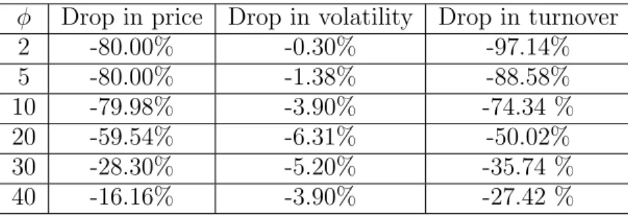
To complete our numerical exercises, we assume that the fundamental component ac-counts for 20% of the pre-lock-up price (this is given by a parameter a) and that the bubble component accounts for the remaining 80% (1−a). If we let k1 = 10 andk2 = 25, so that the float is 2.5 times as big after lock-up as before. Then we get a price drop, defined as the ratio of the after lock-up price to the price before minus one, of approximately 60%, a volatility drop of 6.3% and a drop in expected turnover of 50%. Then we go on to vary four of these parameters, k2, φ, h and a. The results are described more carefully in the Appendix. Of course, our results depend on how big a part of the initial price the bubble component accounted for in the first place. Since a number of these parameters such as a
are difficult to calibrate, we cannot draw strong conclusions from these numerical exercises. Nonetheless, the numerical exercises do illustrate, for many different parameter ranges, that
we are able to get relatively big drops in price and turnover along with a more modest drop in volatility. These exercises suggest that the mechanisms we are describing are indeed capable of generating magnitudes in the ball-park of the those seen during the bursting of the internet bubble.
5.2 Price change across the lock-up expiration date
Another outstanding stylized fact regarding internet stocks during the late nineties involve price dynamics across the lock-up expiration date. Empirical evidence suggests that stock prices tend to decline on the day of the event (see Brav and Gompers (2003), Field and Hanka (2001) and Ofek and Richardson (2000)). This finding is puzzling since the date of this event is known to all in advance.
However, our model is able to rationalize it with the following proposition.
Proposition 6 When the maximum of the two signals sA
I and sBI is larger than the prior
¯
D, the stock price falls on the lock-up expiration date, date (I,2) (i.e. pI,2 < pI,1).
At (I, 1), right before the lock-up expiration at (I, 2), agents from the more optimistic group anticipate that insiders will share their belief after the lock-up expiration. Since insiders are rational (i.e. properly weighing the two public signals), they have a different belief than the overconfident investors. We show that their belief will be lower than that of the optimistic investors. As a result, there will be more selling on the part of insiders on the lock-up expiration date than is anticipated by the optimistic group holding the asset before the lock-up expiration. Hence, the stock price falls on this date.
To demonstrate this, we denote o ∈ {A, B} as the group with the optimistic belief at (I, 1), and ¯o as the other group, (i.e. ˆDo
I ≥ DˆI¯o). Note that the signal overweighted by the
optimistic group (denoted by soI) is higher than the signal overweighted by the pessimistic group (denoted bys¯o
I). Based on the beliefs of overconfident investors in equations (31) and
optimistic investors’ belief and insiders’ belief as ˆ DIo−DˆIin=τ φ τ − 1 τ0+ 2τ ! (soI −D¯) +τ 1 τ − 1 τ0+ 2τ (soI¯−D¯). (53) We show that ˆ DoI−DˆinI ≥ (φ−1)τ0τ τ(τ0+ 2τ) (soI −D¯). (54) When so
I > D¯, it follows that the belief of the optimistic group will be higher than the
insiders’. However, price is a non-linear function of this difference in beliefs because of short-sales constraints. So it does not immediately follow that price drops on date (I, 2). But it turns out that price indeed drops on this date (i.e. pI,2 < pI,1) as a result of this difference.
Studies typically find that among IPOs, around sixty-percent of them exhibit negative abnormal returns on the lock-up expiration date (see, e.g., Brav and Gompers (2003)). This figure can be rationalized by our model. Since the signalssA
I andsBI are symmetrically
distributed around ¯D(in objective measure), it follows that if we were to draw these signals infinitely many times (assuming independence in the cross-section), over fifty percent of the time, the maximum of the two signals will be greater than ¯D. Indeed, we can derive the probability of this as P r[max(sAI, sBI)>D¯] = P r[max(DI−D¯ +AI, DI−D¯+BI)>0] = 1−P r[DI−D¯ +AI ≤0, DI−D¯ +BI ≤0] = 3 4− 1 2πArcT an ρ √ 1−ρ2 ! (55) where ρ, the correlation parameter between sA
I and sBI, is given by
ρ= τ
τ0+τ
. (56)
This correlation parameterρis between 0 and 1. Asρincreases from 0 to 1, the probability decreases from 75% to 50%. Needless to say that the sixty-percent figure found in empirical studies fits comfortably within these bounds.
5.3 Float and the cross-section of expected returns
One of the main predictions of our model is that a stock with a limited float to risk-bearing capacity will have a larger price bubble and hence a lower expected return going forward. In reality, stocks with a low ratio of float to risk bearing capacity may be easier to arbitrage and hence may exhibit less mis-pricing. For instance, one proxy for the ratio of float to risk-bearing capacity might be the market capitalization or the analyst coverage of a stock. And one often thinks that large stocks are indeed easier to arbitrage than small stocks.
So, more interesting from our perspective is that even controlling for firm size (i.e. the total number of shares and risk-bearing capacity), our model predicts that the float of a stock will have an independent effect on expected return. In other words, in our model, float is not simply a proxy for the size of a stock. The reason float matters is that, as we showed in Theorem 2, the very event of potential insider selling at the end of the lock-up period leads to a larger bubble than would have otherwise occurred. As a result, we have the following proposition:
Proposition 7 Even controlling for asset supply and risk bearing capacity (i.e. firm size), a stock with a limited float and hence a greater potential for insider selling will have a larger bubble and hence a lower expected return.
The exact magnitude of the expected return also depends on σl, the volatility of the
difference in beliefs across investors. As we discussed in Proposition 5, for a given increase in float, the drop in the bubble component increases withσl. Cross-sectionally, σl is positively
related to the rate of share turnover (Proposition 3). Hence, after controlling for the increase in asset float, firms with greater share turnover ought to have lower expected returns.
6
Conclusion
In this paper, we develop a discrete-time, multi-period model to understand the relationship between the float of an asset (the publicly tradeable shares) and the propensity for
spec-ulative bubbles to form. Investors trade a stock that initially has a limited float because of insider lock-up restrictions but the tradeable shares of which increase over time as these restrictions expire. They are assumed to have heterogeneous beliefs due to overconfidence and are short-sales constrained. As a result, they pay prices that exceed their own valuation of future dividends because they anticipate finding a buyer willing to pay even more in the future. This resale option imparts a bubble component in asset prices. With limited risk absorption capacity, this resale option depends on float as investors anticipate the change in asset supply over time and speculate over the degree of insider selling.
Our model yields a number of empirical implications that are consistent with stylized accounts of the importance of float for the behavior of internet stock prices during the late nineties. These implications include: 1) a stock price bubble dramatically decreases with float; 2) share turnover and return volatility also decrease with float; and 3) the stock price tends to decline on the lock-up expiration date even though it is known to all in advance.
One potentially interesting avenue for future work is to embed our trading model into a more general model of initial public offerings in which the lock-up and offer price is endogenized. Doing so would allow us to address additional issues such as why we observe pricing in initial public offerings. For instance, in the context of our model, under-pricing, to the extent it attracts a greater number of market participants to the stock, may make sense for insiders. In our model, more investors means better risk-sharing and hence naturally leads to a bigger bubble. More investors may also mean bigger divergence of opinion, which again means a bigger bubble.15 We leave the clarification of these issues for future work.
15
Appendix
7
Proofs
7.1 Proof of Lemma 1
See DeGroot (1970).
7.2 Proof of Lemma 2
Proof follows from substituting in the equilibrium price into demands given in equation (6) and checking that the market clears.
7.3 Proof of Theorem 1
To derive the expectation of B-investors about p1, we directly use equation (13): EB0[p1] = EB0[ ˆf B 1 ]− Q 2ητ −E B 0 " Q 2ητI{l1<−ητQ} # + EB0 " l1 2I{−ητQ<l1< Q ητ} # +EB0 " l1− Q 2ητ ! I{l 1>ητQ} # (A1) Since l1 has a symmetric distribution around zero, we obtain that
EB0 " Q 2ητI{l1<−ητQ} # = EB0 " Q 2ητI{l1>ητQ} # , (A2) and EB0 " l1 2I{−ητQ<l1< Q ητ} # = 0. (A3)
It is direct to verify equation (16).
7.4 Proof of Proposition 1
Define K = ητQ. Note that l1 has a normal distribution with zero mean and a variance of
σ2
l. Thus, we have
= Z ∞ K dl(√l−K) 2πσl e − l2 2σ2 l = σl " 1 √ 2πe −K2 2σ2 l − K σl N(−K/σl) # . (A4)
If we write B =B(Q, η, τ, σl), direct differentiation ofB with respect to Q yields
∂B/∂Q=− 1 ητN − Q ητ σl ! <0. (A5)
Similarly, one can show that ∂B∂η >0, ∂B∂τ >0, and ∂σ∂B
l >0.
The size of the bubble also depends on investor overconfidenceφ, the determinant of the underlying asset – the difference in beliefs. φhas two effects on the speculative components. First, the volatility ofl1 increases withφ. It is direct to verify that σ2l in equation (15)
strictly increases with φ:
∂σ2 l ∂φ = τ(φ−1)[(2φ2+φ+ 1)τ0+ (φ+ 1)(3φ+ 1)τ] φ2[τ 0+ (1 +φ)τ]3 >0. (A6)
Second, an increase inφraises the belief precisionτ, which in turn raises the payoff function for resale options at t= 1. Therefore, the speculative component increases with φ.
7.5 Proof of Proposition 2
Direct differentiation yields
∂2B ∂Q2 = 1 √ 2πη2τ2σ l e− Q2 2η2τ2σ2 l >0. (A7)
Thus, B is convex with respect to Q. It is direct to see that∂B/∂Q is always negative. Its magnitude |∂B/∂Q|peaks at Q= 0 with a value of 2ητ1 , and it monotonically diminishes as
Q becomes large.
The asset price elasticity with respect to share supply, from equation (17), is given by
Q p0 ∂p0 ∂Q =− Q p0 " Σ +Q∂Σ/∂Q 2η + 1 2ητ +|∂B/∂Q| # . (A8)
For two otherwise comparable firms,i.e., they share identicalQ,p0,η, Σ and∂Σ/∂Q, except that one has the bubble component in price, then this firm also has a greater price elasticity to asset supply.
7.6 Proof of Proposition 3
At t = 0,xA0 =xB0 =Q/2. We define the trading volume att = 1 by |xA1 −xB1|/2, and the share turnover rate by
ρ0→1 =
|xA1 −xB1|
2Q . (A9)
By using our discussion of the equilibrium at t = 0 above, we can show
ρ0→1 = 1 2 if fˆ A 1 −fˆ1B > Q ητ ητ 2Q|fˆ A 1 −fˆ1B| if |fˆ1A−fˆ1B| ≤ Q ητ 1 2 if fˆ A 1 −fˆ1B <− Q ητ (A10) Defineh= ητQ( ˆfA 1 −fˆ1B). Then, ρ0→1 = 1 2 if h >1 |h| 2 if −1≤h≤1 1 2 if h <−1 (A11)
Using equations (4) and (5), we obtain
h = η(φ−1)
Q τ(
A
f −Bf). (A12)
Thus, h has a normal distribution with a zero mean and a variance of
σ2h = 2η
2(φ−1)2τ
Q2 (A13)
in the objective probability measure. Then, direct integration provides that
E0[ρ0→1] = σh √ 2π 1−e − 1 2σ2 h ! +N(−1/σh) (A14)
It is easy to see that asQincreases, the distribution of hbecomes more centered around zero. In the mean timeρ0→1 has a bigger value away from zero, therefore E0[ρ0→1] decreases with Q. Intuitively, when more shares are floating, it takes a bigger difference in beliefs