Explainable and Advisable Learning for Self-driving Vehicles

(1)

UC Berkeley

UC Berkeley Electronic Theses and Dissertations

Permalink https://escholarship.org/uc/item/1b97h2dg Author Kim, Jinkyu Publication Date 2019 Peer reviewed|Thesis/dissertation

eScholarship.org Powered by the California Digital Library University of California

(2)

by Jinkyu Kim

A dissertation submitted in partial satisfaction of the requirements for the degree of

Doctor of Philosophy in Computer Science in the Graduate Division of the

University of California, Berkeley

Committee in charge: Professor John Canny, Chair

Professor Trevor Darrell Professor David Whitney

(3)

The dissertation of Jinkyu Kim, titled Explainable and Advisable Learning for Self-driving Vehicles, is approved:

Chair Date

Date

(4)

(5)

1

Abstract

Explainable and Advisable Learning for Self-driving Vehicles by

Jinkyu Kim

Doctor of Philosophy in Computer Science University of California, Berkeley

Professor John Canny, Chair

Deep neural perception and control networks are likely to be a key component of self-driving vehicles. These models need to be explainable - they should provide easy-to-interpret ra-tionales for their behavior – so that passengers, insurance companies, law enforcement, de-velopers, etc., can understand what triggered a particular behavior. Explanations may be

triggered by the neural controller, namely introspective explanations, or informed by the

neural controller’s output, namelyrationalizations.

Our work has focused on the challenge of generating introspective explanations of deep

models for self-driving vehicles. In Chapter 3, we begin by exploring the use of visual

explanations. These explanations take the form of real-time highlighted regions of an image that causally influence the network’s output (steering control). In the first stage, we use a visual attention model to train a convolution network end-to-end from images to steering

angle. The attention model highlights image regions thatpotentially influence the network’s

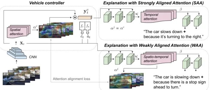
output. Some of these are true influences, but some are spurious. We then apply a causal filtering step to determine which input regions actually influence the output. This produces more succinct visual explanations and more accurately exposes the network’s behavior. In Chapter 4, we add an attention-based video-to-text model to produce textual explanations

of model actions, e.g. “the car slows down because the road is wet”. The attention maps

of controller and explanation model are aligned so that explanations are grounded in the parts of the scene that mattered to the controller. We explore two approaches to attention alignment, strong- and weak-alignment.

These explainable systems represent an externalization of tacit knowledge. The network’s opaque reasoning is simplified to a situation-specific dependence on a visible object in the image. This makes them brittle and potentially unsafe in situations that do not match training data. In Chapter 5, we propose to address this issue by augmenting training data with natural language advice from a human. Advice includes guidance about what to do and where to attend. We present the first step toward advice-giving, where we train an end-to-end

(6)

2

vehicle controller that accepts advice. The controller adapts the way it attends to the scene (visual attention) and the control (steering and speed). Further, in Chapter 6, we propose a new approach that learns vehicle control with the help of long-term (global) human advice. Specifically, our system learns to summarize its visual observations in natural language, predict an appropriate action response (e.g. “I see a pedestrian crossing, so I stop”), and predict the controls, accordingly.

(7)

i

(8)

ii

I would like to thank my advisor John Canny for his patience, support, and motivation through my PhD studies. With his guidance, I have been able to discover a research field I am truly passionate about. Additionally, I would like to thank Anca Dragan for serving my qualification committee, Trevor Darrell and David Whitney for serving on both my qualifica-tion and dissertaqualifica-tion committees. I would also like to thank all those who have mentored me through my PhD, in particular Anna Rohrbach, Zeynep Akata, Laura Waller, Brian Barsky, and Ren Ng. I would also like to thank my Phantom AI internship collaborators Chankyu Lee, Hyunggi Cho, Myung Hwangbo, Youngwook Paul Kwon, Jaehyung Choi, and Jihyun Yoon, my Honda Research Institute USA internship collaborators Teruhisa Misu, Yi-Ting Chen, Ashish Tawari, and Chiho Choi, and my Waymo internship collaborators Mayank Bansal, Woojong Koh, and Drago Anguelov.

Throughout my years at Berkeley, I have been fortunate to have so many collaborators at Berkeley: Cecilia Zhang, Ye Xia, Donghan Lee, Biye Jiang, Daniel Seita, Xinlei Pan, Philippe Laban, Forrest Huang, David Chan, Roshan Rao, Suhong Moon, Yang Gao, Dequan Wang, Coline Devin. I would like to thank my friends for providing emotional support: Saehong Park, Yeojun Kim, Kiwoo Shin, Philjoon Kang, Hyungdong Ha, Sangjae Bae, Bumjoon Seo, Wonyeol Lee and Seunghyun Park.

I would also like to thank Samsung Scholarship for a financial support covering both tuition and stipend.

Finally, I would like to thank my family including my father Hangbok, mother Bangyeo, and sister Chohee. Thank you for providing me with everything I needed to succeed in life. Most of all, I would like to thank my wife Hyerin and son Minoo for their supports and love throughout my life in Berkeley. This dissertation is dedicated to you.

(11)

1

Chapter 1 Introduction

Whereas classical AI systems involved carefully-crafted features and representations, one of the new powers of deep learning methods is the ability to learn very effective latent representations from data. Deep neural perception and control networks are likely to be a key component of self-driving vehicles. In Chapter 2, we first explore that these deep learning methods can be integrated into a self-driving vehicle control model. Unfortunately, whereas human-designed feature maps are often easy to understand, deep representations may not be. While there have been some successes in visualizing deep models on image data,

many models remain cryptic. And even among the successes, success is partial: i.e. while

many individual features are interpretable, many others in the same network are not. A deep network such as a visually-driven action policy embodies tacit, situated knowledge. It is represented as a complex set of learned weights and produces action in response to inputs, with a priori no other abstraction or higher explanation.

In Chapter 3, we first explore to make the model interpretable using visual attention. The attention model weights different areas of the image differently and effectively ignores certain areas completely. This can be visualized with a dynamic heatmap. We have observed that visual attention can be integrated into a state-of-the-art vehicle control model without loss of control accuracy. The collateral benefit of using spatial attention is that it is immediately interpretable: areas that are “dark” in the attention map are masked in the middle of the network and can have no effect on its control output. The converse assertion is not sound however: “bright” areas in the attention map are not necessarily the most important for the vehicle’s control behavior. Attention maps (human attention as well) must be conservative in discarding visual input. The goal of attention is to focus on areas of the image that might be important. Only after images are processed, we can infer the actual influence of those images on the full network. So attention maps are likely to generate false positives (to be concrete, the model often attends to foliage where there might be street signs). Therefore, we add an extra layer of causal filtering: the attention map is clustered into spatio-temporal blobs that roughly correspond to objects in the underlying images (they do not have perfect correspondence with objects since we leave it to human observers to interpret them). We then systematically remove each blob in the attention layer by setting the weights to zero

(12)

CHAPTER 1. INTRODUCTION 2

over its support. If there is a significant change in controller output, then the blob is retained in the attention map. If not, it is discarded. A typical reduction in the number of blobs is more than 2x. By doing this we obtain a much more focused (specific) attention map and we know that the blobs that remain do causally affect the controller.

In Chapter 4, we next move to textual explanations. We use the Berkeley DeepDrive-eXplanation (BDD-X) dataset which is constructed the following way. Video from a number of drivers in the United States was collected using small camera devices placed on the dash-board just above the steering wheel. This data was subsequently annotated using Amazon Mechanical Turk where the task was to view the video and provide both a description of the drivers’ actions and then an explanation for them. The turker was asked to put them-selves in the position of a driving instructor providing explanations to a student driver. The explanations obtained in this way are pure rationalizations since they were generated by an observer, not the driver. While it might be more desirable to use self-report data from drivers themselves, the collection of such a dataset poses a number of challenges. For now we have used the existing Berkeley DeepDrive-Video (BDD-V) dataset, which has the advantage that we at least do not need to determine whether human explanations are based on true introspection or rationalization since it is always the latter for this dataset. We use this data to train an explanation generator. It remains for us to try to generate explanations that are grounded in the model’s actual behavior even though there is no such information in the training dataset. We return again to spatial attention – our controller has already high-lighted regions in the image that affect its output using its own attention map augmented by causal filtering. Spatial and temporal attention has also been successfully applied for generating text annotations of videos. That is, the explanation module also highlights the areas of the video that it used in its explanations. These two attention models should align in an appropriate sense: The explanation module should not causally attend to regions of the image that did not causally affect the controller output. In other words, the explanation module’s causal attention map should be a subset of the controller’s. We have to take care in dealing with time – the controller’s “time” is the same as the timestamp in the video stream. A grammatical explanation will often generate words (and attend to corresponding image regions) in a quite different order from their prominence for the controller. Thus our two attention maps are compared using a metric which allows flexibility in temporal alignment. These explainable systems represent an externalization of tacit knowledge. The network’s opaque reasoning is simplified to a situation-specific dependence on a visible object in the image. It is better considered as part of socialization, where explanations are offered in a master-apprentice context with the control policy serving as an instructor. We explore advisable AI systems that are built directly on our work on explanations. The explainable driving model project has connected with a number of industry researchers through the Berkeley Deep Drive initiative. From them, and from other prospective users we have had a lot of feedback about the need for users not only to understand the driving controller, but to influence it. Since users are typically not paying attention to the vehicle’s detailed behavior, such influence should be high-level. We use the term “advisable AI” to convey the notion of partnership between human and machine. It contrasts with commanding, or

(13)

CHAPTER 1. INTRODUCTION 3

even constraining the robot’s actions. It is a form of user customization, although it is typically quite dynamic since the user’s preferences for driving behavior are likely to change frequently. Human-to-vehicle advice can take a variety of forms, with different levels of

urgency, e.g. “drive more slowly/gently”, “Avoid roads with speed bumps”. Some of these

are commands that should always be followed. Markers such as “always”, “don’t” “avoid” indicate that the user expects their directions to be followed.

In Chapter 5, we observe that deep neural control networks, which are trained on large datasets to imitate human actions, lack semantic understanding of image contents. This makes them brittle and potentially unsafe in situations that do not match training data. We propose to address this issue by augmenting training data with natural language advice from a human. Advice includes guidance about what to do and where to attend. We present a first step toward advice giving, where we train an end-to-end vehicle controller that accepts advice. The controller adapts the way it attends to the scene (visual attention) and the control (steering and speed). Attention mechanisms tie controller behavior to salient objects in the advice. We evaluate our model on a novel advisable driving dataset with manually annotated human-to-vehicle advice called Honda Research Institute-Advice Dataset (HAD). We show that taking advice improves the performance of the end-to-end network, while the network cues on a variety of visual features that are provided by advice. This was the first paper on the use of advice, but this design is most appropriate for turn-by-turn (short duration) advice. Since our data comprised short clips, advice was effective throughout the clip. It will be worth exploring other styles of advice, such as per-ride advice (gentle, fast, etc) and rule-based global advice.

In Chapter 6, we propose to use human advice in the form of observation-action rules. Specifically, we propose a new approach that learns vehicle control with the help of human advice. Specifically, our system learns to summarize its visual observations in natural

lan-guage, predict an appropriate action response (e.g. “I see a pedestrian crossing, so I stop”),

and predict the controls, accordingly. Moreover, to enhance interpretability of our system, we introduce a fine-grained attention mechanism which relies on semantic segmentation and object-centric RoI pooling. We show that our approach of training the autonomous system with human advice, grounded in a rich semantic representation, matches or outperforms prior work in terms of control prediction and explanation generation. Our approach also results in more interpretable visual explanations by visualizing object-centric attention maps.

(14)

4

Chapter 2 Deep Traffic Light Detection for

Self-driving Cars from a Large-scale

Dataset

2.1 Problem Statement

Traffic lights detection problem is one of the key challenges for autonomous vehicle controllers in urban areas. While a number of approaches for traffic light detection have been proposed, these methods often require a prior knowledge of map and/or show high false positive rates. Recent successes suggest that deep neural networks will be widely used in self-driving cars, but current public datasets do not provide sufficient amount of labels for training such large deep neural networks. In this paper, we developed a two-step computational method that can detect traffic lights from images in a real-time manner. The first step exploits a deep neural object detection architecture to fine true traffic light candidates. In the second step, a point-based reward system is used to eliminate false traffic lights out of the candidates. To evaluate the proposed approach, we collected a human-annotated large-scale traffic lights dataset (over 60 hours). We also designed a real-world experiment with an instrumented self-driving vehicle and observed that the proposed method was able to handle false traffic lights substantially better compared with the baseline considered.

Self-driving vehicle control has recently made remarkable progress. These controllers in-volve a variety of sophisticated algorithms for perception, behavioral/motion planner, and

dynamics controllers. Despite their recent success in some driving scenarios (i.e. highway

driving), there still remain new challenges for urban driving that involves more complex driv-ing scenarios that need interaction with traffic controls, vehicles, pedestrians, etc. Especially, *This work has been presented at the 20th IEEE International Conference on Intelligent Transportation Systems (ITSC), 2017.

(15)

CHAPTER 2. DEEP TRAFFIC LIGHT DETECTION FOR SELF-DRIVING CARS

FROM A LARGE-SCALE DATASET 5

In p u t im a g e s V is u a li za ti o n o f d e te c ti o n s time Spatiotemporal Filtering

Vehicle Motion Planner PID Controller Coarse-grained detector (acceleration, steering) Detections / Decision Traffic light candidates Candidates Buffer

RED

Figure 2.1: Our model detects traffic lights,e.g. a red circle, from an input raw image at each

timestep. Our model consists of two major steps: (1) coarse-grained detector that utilizes deep neural object detection architecture and is tuned to discover as many true traffic lights as possible. (2) the spatiotemporal filtering step that eliminates false traffic lights with respect to features extracted from both spatial and temporal domains. The output of our proposed detector is then fed into the vehicle motion planner and the PID controller that computes corresponding acceleration and steering angle commands.

traffic lights pose a challenging (computer vision) problem when subject to varying lighting, view distances, and weather conditions. Though its importance for automated driving in ur-ban areas, conventional approaches showed insufficient reliability and robustness enough to be used in autonomous systems in the urban environment without utilizing prior knowledge. Recent successes suggest that deep neural networks will be widely used in self-driving

cars, especially for a perception part. Behrendt et al. [8] utilized the “You Only Look Once”

(YOLO) network architecture followed by a small classification convolutional network to detect traffic lights. For obtaining a reliable and robust performance from such a large deep neural network, a large amount of dataset is strongly required to provide a large variation in environmental conditions. However, the current publicly available datasets show lacks such variation. For example, the VIVA challenge [62] for traffic lights only provide 44 minutes of data and the Bosch Small Traffic Lights Dataset [8] provides only about 5,000 images (less than 3 hours), which is insufficient from the view of the conventional way of training

(16)

such large deep neural networks. We, therefore, create a large dataset, which provides over

60 hours of driving images that cover diverse driving conditions (i.e. lighting and weather).

Thus, we argue this dataset will be ideal for further traffic light detection studies.

Collecting a large-scale dataset is only part of a story. Reliable traffic light detector strongly requires low false negative (or discovering as many true traffic lights as possible) and false positive (or eliminating false traffic lights) rates, while maintaining a high detection accuracy. Here, we propose a new computational method for traffic light detection, which consists of two major steps: (1) coarse-grained traffic light detection and (2) spatiotemporal filtering of the detected traffic lights. The first step considers individual images and collects traffic light candidates using a deep neural object detection architecture. The focus of this step is to reduce false negatives (FNs) or to discover as many true traffic lights as possible. The second step is then to eliminate false positives (FPs) by considering spatial and temporal characteristics of traffic lights. To distinguish true and false traffic lights, we propose a point-based reward system where each detected traffic lights earn rewards and the final decision is made based on these rewards. To demonstrate the effectiveness of applying the proposed method to self-driving vehicles, we test with an instrumented vehicle and successfully drive 6 kilometers on city streets in the San Francisco Bay Area, California, USA.

Our contributions can be summarized as follows: (i) We propose a new computational method for accurately detecting traffic lights from a raw input image in a real-time manner. (ii) We generated a large-scale traffic lights dataset with over 71,771 images (over 60 hours) with human annotated bounding boxes. (iii) We demonstrate the effectiveness of applying our proposed approach by conducting a real-world experiment (driving over 6 kilometers including 17 intersections with traffic lights) with an instrumented vehicle.

2.2 Deep Traffic Light Detection Model

Here, we propose a method that accurately and reliably detects traffic lights from a stream of images captured by a front-view dash-cam attached to the windshield. As we depicted in Figure 2.2, the proposed method contains two major steps: (1) coarse-grained traffic light detector and (2) spatiotemporal filtering of the traffic lights candidates. In the first step (coarse-grained detector), traffic light candidates from each image are collected by utilizing a deep neural object detection architecture. The main focus of this step is to discover

the true traffic lights as many as possible (i.e. reducing the number of false negatives).

Thus, it is possible that the traffic light candidate collection may contain false positives. In the second step (spatiotemporal filtering), we eliminate such erroneously detected traffic lights by simultaneously considering other traffic lights over time and space. To distinguish between true and false traffic lights, we use a point-based reward system where each detected traffic lights earn rewards with respect to features extracted from both spatial and temporal domains.

(17)

Input image (1280x720@30Hz) Output visualization Our instrumented vehicle

1. Coarse-grained detector: SSD 2. Spatiotemporal refinement

3 512 288 128 1 1 9 16 256 3 3 9 16 128 1 1 5 8 256 3 3 5 8 Preprocessing Visualizer VGG-16 (through conv5_3) 1 1 18 36 64 32 256 stride of 1 stride of 1 stride of 1 stride of 2 stride of 2 3 3 18 32 512 512 c on v4_3 D e te ct io n s N o n -ma xi mu m Su p p re ssi o n conv 3x3 conv 3x3 conv 3x3 conv 3x3 Labels Message passing on ROS @30Hz Candidates Fine-grained detector Score computation Decision maker 3 . V e h ic le c o n tr o lle r

Vehicle motion planner PID controller

Outputs:

vehicle control commands

UNK GREEN

Figure 2.2: An overview of our proposed model. It can be understood in three parts: (i) a coarse-grained detector that utilizes the deep neural perception network architecture called SSD (Single-Shot multi-box Detector [50]), (ii) a spatiotemporal filtering, and (iii) a vehicle controller. To demonstrate the feasibility of applying our model to self-driving cars, we use an instrumented autonomous vehicle which uses the output of our model as an input to control its dynamics.

2.2.1 Preprocessing

We use an input image that is resized to 288×512×3 with bilinear interpolation algorithm,

hence to reduce computational burdens for a real-time detection. For the images with dif-ferent aspect ratios, we cropped the height to match the ratio. Following a common practice in image classification tasks, we subtracted the mean RGB value to achieve zero-centered inputs, which are originally in different scales. Note that our dataset contains images where the camera gains are automatically calibrated to obtain high-quality images. During the testing process, we also used a cropped image in the center part of the image, where traffic

lights are commonly observed in that area. Thus, a batch of two images (i.e. whole and

(18)

2.2.2 Coarse-grained Traffic Light Detection

Traffic light detector strongly requires showing reliable performance in real-time and working

for both small (i.e. 3×9 pixels) and large objects with low false positive and low false negative

rates, while maintaining a high detection accuracy. For example, a false red traffic light will lead the autonomous vehicle to abruptly stop while driving, while a missed red light will cause the vehicle to go through an intersection originally with red lights in its course of driving.

In this coarse-grained traffic light detection step, we focus to reduce false negative (FN) rates or to collect as many true traffic lights as possible. We utilize the Single-Shot multi-box Detector (SSD) [50] that has been shown to be an effective tool for an object detection task. Note that we use the SSD architecture that has shown improved detection accuracy in other benchmarks than YOLO network architecture, which was utilized in the existing work

by Behrendt et al. [8]. More modern architecture, such as Mask R-CNN [25], may provide

better detection accuracy, but we leave this comparison for future work. The SSD model is based on a convolutional network and takes the whole image as an input and predicts a fixed-size collection of bounding boxes and corresponding confident scores for the presence of object instances in those boxes. The final detections are then produced followed by a non-maximum suppression step – all detection boxes are sorted on the basis of their predicted scores, and the detections with maximum score is then selected, while other detections with a significant overlap are suppressed. As we described in Figure 2.2, we use a standard VGG-16 network architecture [72] as a base convolutional network, which is pre-trained on ImageNet Large Scale Visual Recognition Challenge (ILSVRC) dataset [69]. Auxiliary structures – convolutional predictor and the additional convolutional feature extractor – are

used following the work by Liu et al. [50].

2.2.2.1 Training Objective.

The loss functionL(=Lloc+Lconf) is a weighted sum of two types of loss: (1) the localization

loss Lloc measures a SmoothL1 loss between the predicted and the ground-truth bounding

box in a feature space. (2) The confidence loss Lconf is a softmax loss over multiple classes

confidences. For more rigorous details, refer to Lieet al. [50].

2.2.2.2 Data Augmentation.

To train a robust detector to various object sizes, we use random cropping (the size of each sampled image is [0.5, 1] of the original image size with fixed aspect ratio) and flipping to

yield consistent improvement. Following the work by Liuet al. [50], we also sample an image

so that the minimum Jaccard overlap with the objects is {0.1, 0.3, 0.5, 0.7, 0.9}. Note that

each sampled image is then resized to a fixed size followed by photometric distortions with respect to brightness, contrast, and saturation.

(19)

2.2.3 Characterizing Traffic Lights

According to our analysis, the traffic lights appearing in the detection pipeline possess the following characteristics:

(C.1) As the confidence of a traffic light candidate decreases, so does the possibility of this being a true traffic light.

(C.2) The possibility of a traffic light candidate being true increases if the traffic light can-didate is detected again in next timestep at almost the same location.

(C.3) If multiple traffic lights of the same category (i.e. red, yellow, and green) are detected

in a scene, then they are usually true traffic lights differently located (i.e. multiple

traffic lights are installed at an intersection).

(C.4) Traffic lights shall be located following the governmental guideline (i.e. at least one of

the signal faces shall be located at an intersection mounted on the mast arm.), hence the possibility of a traffic light candidate being true increases as its location gets close to the usual.

As is evident above, examining traffic lights individually is not sufficient, and multiple traffic light candidates over space and time should be considered simultaneously.

2.2.4 Spatiotemporal Filtering

2.2.4.1 Fine-grained Detector

Recall from Section 2.2.1, we re-scaled images by 40% to reduce the computational burdens for a real-time system. We observe that the classification performance of our coarse-grained

detector slightly decreases as we have smaller traffic lights (i.e. seen from a farther distance).

Thus, we utilize an additional small classification network, called fine-grained detector, that has a high-resolution input. All bounding boxes from the coarse-grained detector are cropped

and rescaled to 100×100 pixels, they are then fed into the fine-grained detector. For

train-ing, we collect image patches that are cropped and rescaled from the ground-truth dataset. Overall, we collect 24,991 and 6,248 patches for training and validation, respectively.

2.2.4.2 Score Function

According to our traffic light characterization (see C.1–C.4), we need to examine multiple traffic light candidates simultaneously for accurate traffic light status recognition. In addi-tion, we set the confidence threshold value of the coarse-grained detector so as to minimize

the number of FNs (i.e. the true traffic lights that are erroneously left undetected).

Conse-quently, it is likely that the traffic lights detected in the previous step contain false traffic lights that further need to be filtered out. In this spatiotemporal filtering step, we seek to

(20)

resolve these issues using a point-based reward system where each detected traffic lights earn points with respect to the following characterizations:

(S.1) Each traffic light candidate has its own score for being true, and its score is accumulated

in the next timestep if detected again under our matching criterion (i.e. euclidean

distance between centers of each candidate).

(S.2) Every traffic light candidates from coarse-grained detector earn a reward R at each

timestep.

(S.3) Scores are discounted by a pre-specified discount rate γ at each timestep.

Concretely, the score function sj(t) for a candidate j is defined as follows:

sj(t) = min Smax, Rcj(t) +γsj(t−1)

(2.1)

where cj(t) ∈ [0,1] is the confidence value computed by the coarse-grained detector. A

maximum score is set toSmax.

2.2.4.3 Decision

The output of this step is a tuple of the current traffic light status. For each typek of traffic

light signals (i.e.k ∈{turning left, going forward, turning right}) and each traffic light status

(i.e. unknown, red, yellow, and green), we accumulate scores over traffic light candidates and

output the status of the maximum score.

ok(t) =argmaxi∈{red, yellow, green, unknown}

X

j

1(i, j)sj(t) (2.2)

where ₁(i, j) is an indicator function that is 1 if j-th candidate has the same status as i,

otherwise 0.

2.3 Dataset

In order to effectively train and evaluate a deep neural perception approach, we have col-lected a large-scale traffic lights dataset. Our dataset contains RGB color images captured by a dashcam mounted behind the front mirror of the vehicle. Each image has the resolution

of 1280×720 pixels. We provide the dataset statistics in Table 2.1. Our dataset is composed

of over 60 hours of driving taken in diverse driving conditions,e.g. day/night, city/residential

ares, etc. We have collected 71,771 images mainly in the San Francisco Bay Area in Cali-fornia, USA. To avoid high similarity between images, we sample images at every 3 seconds. Overall, 34,604 are labeled, the minimum size of labeled traffic lights is approximately 3

(width)×9 (height) pixels. We also introduce a training and a test set, containing 64,607

and 7,164 images, respectively. In Figure 2.3, we illustrate the distribution of the different traffic light states, which have eight categories: off, too small to annotate, green (circle), red (circle), yellow (circle), green (left-turn), red (left-turn), and yellow (left-turn).

(21)

2.4 Experiments

2.4.1 Training and Evaluation Details

For training a coarse-grained detection model, we use the stochastic gradient algorithm (SGD). Unless stated, we use default hyper-parameters following the work by Liu [50]. Our model took less than 3 days to train on three NVIDIA Titan X Pascal GPUs. Our imple-mentation is based on a deep learning framework called Caffe [35].

2.4.2 Quantitative Analysis

As shown in Figure 2.4, we first measured the classification performance of our coarse-grained traffic light detector in terms of recall and precision. We tested with different threshold values in [0, 1]. Note that a good classifier will have higher precision and recall values. The coarse-grained detector seeks to minimize the number of FNs (or undetected true traffic lights) to maintain high recall – suggesting that few true traffic lights went undetected by using this method. In the cases tested, maintaining a high recall increases the number of FPs (or detected false traffic lights), which support the need to use the refinement step. The numbers of training example for the yellow circle and left lights are smaller than other colors, and we observe the classifier shows poor classification performance for the yellow circle and left lights. It would also worth exploring the use of other types of more expressive neural networks, which may give a performance improvement over our network configuration [32]. However, exploration of other architectures would be out of our scope.

Table 2.1: Dataset details with the comparison to other publicly available datasets: the VIVA Challenge for traffic lights [62] and the Bosch Small Traffic Lights dataset [8].

VIVA [62] Bosch [8] Ours

Training Testing Training Testing Training Testing

#Images 20,526 22,481 5,093 8,334 64,607 7,164

FPS 16 16 1/2 15.6 1/3 1/3

#Annotations 54,161 64,170 10,756 13,493 31,239 3,365

#Hours ≈22min ≈ 22min ≈ 2.8 hours ≈ 8.9min ≈ 53 hours ≈6 hours

Image Res. 1280×960 1280×720 1280×720

(22)

12,000

N

u

m

b

e

r

o

f

a

n

o

ta

ti

o

n

s

10,000

8,000

6,000

4,000

2,000

10,797 #Training Training #Testing Testing 1,980 7,649 2,790 143 977 4,445 2,458 1,376 83 964 311 8 62 445 116 Too small

0

Figure 2.3: Traffic lights annotation statistics.

Recall from Section 2.2.4, we use a fine-grained detector that further examines the traffic light candidates by using an additional small neural network with high-resolution inputs. Table 2.2 shows the classification performance with and without the fine-grained detector.

In the cases tested except for two classes (i.e. red circle and red left), using a fine-grained

detector resulted in higher classification performance in F-measure values. The F-measure is 3.44 - 17.03% higher as compared to the coarse-grained detector only.

2.4.3 Real-world Experiments

To demonstrate the feasibility of applying our traffic light detector for a real self-driving car (see Figure 2.5 (A)), we utilize an instrumented vehicle equipped with the following specifications:

(V.1) Vehicle: Hyundai Genesis G80

(V.2) Sensors: 2×Velodyne LiDAR sensors, 4×Radar sensors, and 1×video camera

(resolu-tion: 1280x720 pixels, frame rate: 10Hz, field of view (FOV): 60 degrees).

(V.3) PC: Intel i7 Quad-core processor, 16GB DDR3 memory, a 1TB SSD, a Titan X Pascal GPU, and Linux OS.

(23)

Green circle Red circle Yellow circle 0.0 0.0 0.2 0.4 0.6 0.8 1.0 0.2 Recall Pr e c is io n 0.4 0.6 0.8 1.0 Green left Red left Yellow left 0.0 0.0 0.2 0.4 0.6 0.8 1.0 0.2 Recall Pr e c is io n 0.4 0.6 0.8 1.0

A

B

Figure 2.4: Performance evaluation of our coarse-grained detector in terms of two widely-used metrics: precision and recall. For red, green, and yellow circles, see A. For others, see B.

We use the Robot Operating System (ROS) for synchronizing the sensor data and for the message passing of perception, motion planning, and control nodes. At each timestep, the sensory data is consumed from raw sensors (camera, LiDAR, and Radar) and processed by a collection of ROS nodes that all communicate with each other. We use the PID controller for our control node, hence the final output control commands to the throttle, brake, and Table 2.2: The effect of using fine-grained detector (see Section 2.2.4) is evaluated in terms of precision, recall, and F-measure. Scores are reported in percentage (%).

Classes

without

Fine-grained detector

with

Fine-grained detector

Precision Recall F-measure Precision Recall F-measure

Red circle

70.20

29.70

41.74

68.00

29.50

41.15 Yellow circle

2.20

40.00

4.17

6.00

30.90

10.05 Green circle

37.60

87.80

52.65

60.80

81.60

69.68 Red left

84.20

27.70

41.69

62.40

29.00

39.60 Yellow left

14.30

8.30

10.50

66.70

16.70

26.71 Green left

32.30

50.00

39.25

36.40

51.60

42.69

(24)

A B C D E Start point Intersection

with traffic lights End point Start/end points

The San Francisco Bay Area, CA, USA

Testing route

Velodyne LiDAR sensors Radar sensors High-res. Camera

GREEN GREEN GREEN RED GREEN RED

+22 sec +20 sec +18 sec +16 sec +14 sec +12 sec +10 sec +8 sec +6 sec +4 sec +2 sec +0 sec +10 sec +8 sec +6 sec +4 sec +2 sec +0 sec UNK UNK UNK UNK UNK UNK

Figure 2.5: (A) Our instrumented vehicle with sensor layout for real-world evaluation of the proposed traffic light detection pipeline. (B) Our testing route (in the San Francisco Bay Area, CA, USA) for the real-world experiment. This route is over 6 kilometers including 17

intersections with traffic lights installed. Map credit: Google Maps. (C-D) Visualizations

for traffic light detection over time. Unseen consecutive input images are sampled at every 2 seconds (see bottom-right). Our final decisions are depicted on the top of each figure, while detected traffic lights are highlighted by a white circle. (E) Additional examples of detected traffic lights during the test scenario.

(25)

steering wheel are provided through our drive-by-wire units. We depict major steps in

Figure 2.2.

We test our proposed traffic light detector with an instrumented vehicle on public roads in Bay Area, California, USA. As shown in Figure 2.5 (C-E), the test runs were performed in an unseen pre-specified testing route (over 6 kilometers), and the test scenario comprised the following features: (1) The vehicle traversed 17 traffic light-controlled intersections where the vehicle will follow the rules to stop on red and go on green. (2) Different lighting conditions (day vs. night), weather (rainy vs. sunny), and different road traffic congestion levels are tested. We build a visualization to show which traffic lights are detected and its the final decision. We provide examples from our visualizer during the on-road driving test. Our real-world experiments support that the proposed traffic light detector can be successfully operated in a real-time manner.

2.5 Related Work

A number of approaches have been proposed for traffic light detection and classification for autonomous vehicles and/or for driver assistance systems to navigate in urban areas. Most of these approaches utilized a supervised learning approach with human-designated features. This literature is too wide to survey here. For a thorough review of this literature, see [34]. These approaches usually depend on strong assumptions: (1) they are based on recog-nizing human-designated features, which generally require demanding parameter tuning for a balanced performance. (2) Some require the detailed maps that provide prior knowledge about the specific locations of all installed traffic lights, which but demand high costs in building such a map. Furthermore, other issues may include: (i) color-tone shifting due to changes in atmospheric conditions and nearby light sources. (ii) Occlusion by other objects. (iii) High false positive rates caused by brake lights, reflections, and pedestrian crossing lights. (iv) Inconsistent traffic light lamps due to dirt, defects, over-saturation of the camera (especially during night-time).

Recent approaches suggest that deep neural networks can be successfully used for the

traffic light detection task. Weber et al. [84] utilized a 7-layer convolutional neural network

to predict the multi-class probability map followed by bounding box regression. Behrendtet

al. [8] used the “You Only Look Once” (YOLO) network architecture to detect traffic lights,

and utilized a tiny convolutional neural network to classify the categories of each detected traffic lights. They also provide a dataset, called the Bosch Small Traffic Lights Dataset, which provides approximately 5,000 images (2.8 hours of driving) and 8,334 annotations. Despite its potential, training these deep neural networks requires a large amount of anno-tated dataset to train a reliable detector that can address challenges in traffic light detection task. Though there exist some other open-sources of traffic light annotations, these datasets are still insufficient for training deep neural networks in terms of diversity of scenes, quality of annotations, and their limited volume. For example, the VIVA challenge dataset [62] only provides approximately 40 minutes of scenes, while the Bosch [8] Small Traffic Lights

(26)

dataset provides less than 3 hours (5,000 images). We, therefore, collect our own dataset, which provides over 60 hours (over 71,771 images) of driving images that cover diverse

driv-ing conditions (i.e. day vs. night and sunny vs. raining). Thus, we argue this dataset will

(27)

17

Chapter 3 Interpretable Learning for

Self-Driving Cars by Visualizing

Causal Attention

3.1 Problem Statement

Self-driving vehicle control has made dramatic progress in the last several years, and many auto vendors have pledged large-scale commercialization in a 2-3 year time frame. These controllers use a variety of approaches but recent successes [9] suggest that neural networks will be widely used in self-driving vehicles. Deep neural networks have been shown to be an effective tool [9, 87] to learn vehicle controls for self-driving cars in an end-to-end manner. Despite their effectiveness as a function estimator, DNNs operate as a black-box – both net-work architecture and hidden layer activations may have no obvious relation to the function being estimated by the network.

(i) Introspective explanations: A system is introspective through a series of

under-standable ways (i.e. Bob explains Bob’s actions).

(ii) Rationalizations: We want to justify or rationalize the system through a series of logically consistent and understandable choices that can correlate model response

with physical observations (i.e. Alice watching a video of Bob, and then asking

Alice to justify Bob’s actions).

*This work has been presented at the 16th IEEE International Conference on Computer Vision (ICCV), 2017.

(28)

CHAPTER 3. INTERPRETABLE LEARNING FOR SELF-DRIVING CARS BY

VISUALIZING CAUSAL ATTENTION 18

Input images Attention heat map _{steering angle}Output

1. Encoder : Convolutional Feature Extraction 2. Coarse-Grained Decoder: Visual Attention

3. Fine-Grained Decoder 3 Stride of 2 Stride of 2 Stride of 2 Stride of 1 Stride of 1 5 5 5 5 160 80 40 80 36 24 3 3 20 40 48 3 3 10 20 64 3 3 10 20 64 10 20 1 10 20 64 t+1 10 20 Preprocessing LSTM

Visual Saliency detection and causality check Clustering analysis 1 1 2 2 3 3 4 4 5 5 6 6 7 7 8 8 (x10 ) 2 3 4 5 6 -5

Figure 3.1: Our model predicts steering angle commands from an input raw image stream in an end-to-end manner. In addition, our model generates a heat map of attention, which can visualize where and what the model sees. To this end, we first encode images with a CNN and decode this feature into a heat map of attention, which is also used to control a vehicle. We test its causality by scrutinizing each cluster of attention blobs and produce a refined attention heat map of causal visual saliency.

To allow end-users understand what has triggered a particular behavior, hence to increase trust, these models need to be self-explanatory. There exist two main types of philosophical argument for explanations [2]: (i) Introspective explanations and (ii) rationalizations.

One way of achieving introspection is via visual attention mechanisms [88]. Visual at-tention filters out non-salient image regions, hence the model visually fixates on important image content that is relevant to the decision. These networks provide spatial attention maps – areas of the image that the network attends to – that can be displayed in a way that is easy for users to interpret. They provide their attention maps instantly on images that are input to the network, and in this case on the stream of images from automobile video. Providing visual attention to the user as a justification of a decision increases trust. As we show from our examples later, visual attention maps lie over image areas that have an intuitive influence on the vehicle’s control signal. Further, we show that state-of-the-art driving models can be made interpretable without sacrificing accuracy, that attention models provide more robust image annotation, and causal analysis further improves explanation saliency.

But attention maps are only part of the story. Attention is a mechanism for filtering

(29)

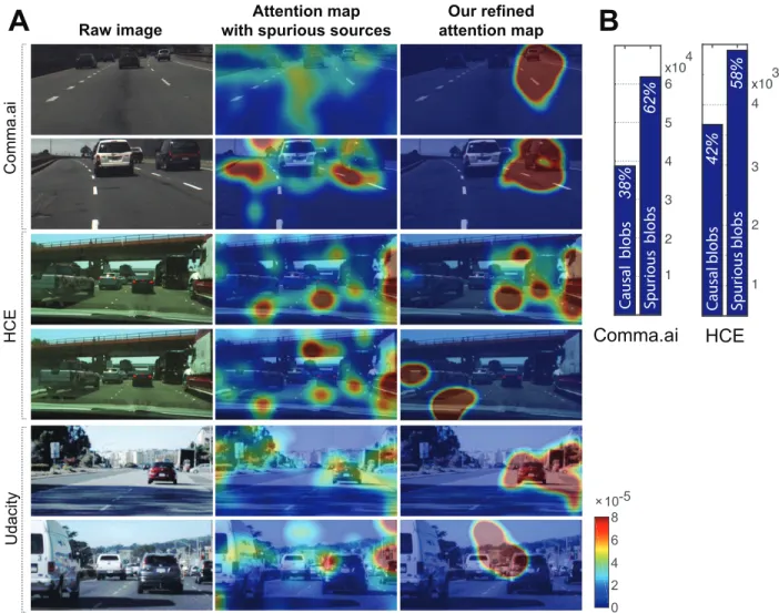
image areas and pass them to the main recognition network (a CNN here) for a final verdict. For instance, the attention network will attend to trees and bushes in areas of an image where road signs commonly occur. Just as a human will use peripheral vision to determine that “there is something there”, and then visually fixate on the item to determine what it actually is. We therefore post-process the attention network’s output, clustering it into attention “blobs” and then mask (set the attention weights to zero) each blob to determine the effect on the end-to-end network output. Blobs that have an causal effect on network output are retained while those that do not are removed from the visual map presented to the user.

Figure 3.1 shows an overview of our model. Our approach can be divided into three steps: (1) Encoder: convolutional feature extraction, (2) Coarse-grained decoder by visual attention mechanism, and (3) Fine-grained decoder: causal visual saliency detection and refinement of attention map. Our contributions are as follows:

• We show that visual attention heat maps are suitable “explanations” for the behavior

of a deep neural vehicle controller, and do not degrade control accuracy.

• We show that attention maps comprise “blobs” that can be segmented and filtered to

produce simpler and more accurate maps of visual saliency.

• We demonstrate the effectiveness of using our model with three large real-world driving

datasets that contain over 1,200,000 video frames (approx. 16 hours).

• We illustrate typical spurious attention sources in driving video and quantify the

re-duction in explanation complexity from causal filtering.

3.2 Interpretable Driving Model

As we depicted in Figure 3.1, our model predicts continuous steering angle commands from input raw images end-to-end. Our model can be divided into three steps: (1) Encoder:

convolutional feature extraction (Section??) (2) Coarse-grained decoder by visual attention

mechanism (Section 3.2.3), and (3) Fine-grained decoder: causal visual saliency detection and refinement of attention maps (Section 3.2.4).

3.2.1 Preprocessing

Our model predicts continuous steering angle commands from input raw pixels in an

end-to-end manner. As discussed by Bojarski et al. [9], our model predicts the inverse turning

radius ˆut (=rt−1, wherertis the turning radius) at every timestep tinstead of steering angle

commands, which depends on the vehicle’s steering geometry and also result in numerical instability when predicting near zero steering angle commands. The relationship between

(30)

the inverse turning radius ut and the steering angle command θt can be approximated by

Ackermann steering geometry [64] as follows:

θt=fsteers(ut) =utdwKs(1 +Kslipvt2) (3.1)

where θt in degrees and vt (m/s) is a steering angle and a velocity at time t, respectively.

Ks,Kslip, and dw are vehicle-specific parameters. Ks is a steering ratio between the turn of

the steering and the turn of the wheels. Ksliprepresents the relative motion between a wheel

and the surface of road. dw is the length between the front and rear wheels. Our model

therefore needs two measurements for training: timestamped vehicle’s speed and steering angle commands.

To reduce computational cost, each raw input image is down-sampled and resized to

80×160×3 with nearest-neighbor scaling algorithm. For images with different raw aspect

ratios, we cropped the height to match the ratio before down-sampling. A common practice in image classification is to subtract the mean RGB value computed on the training set from each pixel simonyan2014very. This is effective to achieve zero-centered inputs which are originally in different scales. Driving datasets, however, do not show that various scales. For instance, the camera gains are (automatically or in advance) calibrated to capture such high-quality images in a certain dynamic range. In our experiment, we could not obtain significant improvement by the use of mean subtraction. Instead, we change the range of pixel intensity values and convert to HSV colorspace, which is commonly used for its robustness in problems where color description plays an integral role.

We utilize a single exponential smoothing method [33] to reduce the effect of human factors-related performance variation and the effect of measurement noise. Formally, given a

smoothing factor 0≤αs ≤1, the simple exponential smoothing method is defined as follows:

_ˆ θt ˆ vt =αs θt vt + (1−αs) _ˆ θt−1 ˆ vt−1 (3.2)

where ˆθt and ˆvt are the smoothed time-series of θt and vt, respectively. Note that they are

same as the original time-series whenαs = 1, while values of αs closer to zero have a greater

smoothing effect and are less responsive to recent changes. The effect of applying smoothing methods is summarized in Section 3.3.4.

3.2.2 Encoder: Convolutional Feature Extraction

We use a convolutional neural network to extract a set of encoded visual feature vector,

which we refer to as a convolutional feature cube xt. Each feature vectors may contain

high-level object descriptions that allow the attention model to selectively pay attention to certain parts of an input image by choosing a subset of feature vectors.

As depicted in Figure 3.1, we use a 5-layered convolution network that is utilized by

(31)

omit max-pooling layers to prevent spatial locational information loss as the strongest acti-vation propagates through the model. We collect a three-dimensional convolutional feature

cube xt from the last layer by pushing the preprocessed image through the model, and the

output feature cube will be used as an input of the LSTM layers, which we will explain in Section 3.2.3. Using this convolutional feature cube from the last layer has advantages in generating high-level object descriptions, thus increasing interpretability and reducing computational burdens for a real-time system.

Formally, a convolutional feature cube of size W×H×D is created at each timestep t

from the last convolutional layer. We then collect xt, a set of L= W ×H vectors, each of

which is a D-dimensional feature slice for different spatial parts of the given input.

xt={xt,1, xt,2, . . . , xt,L} (3.3)

where xt,i ∈ RD for i∈ {1,2, . . . , L}. This allows us to focus selectively on different spatial

parts of the given image by choosing a subset of these L feature vectors.

3.2.3 Coarse-Grained Decoder: Visual Attention

The goal of soft deterministic attention mechanism π({xt,1, xt,2, . . . , xt,L}) is to search for a

good context vector yt, which is defined as a combination of convolutional feature vectors

xt,i, while producing better prediction accuracy. We utilize a deterministic soft attention

mechanism that is trainable by standard back-propagation methods, which thus has advan-tages over a hard stochastic attention mechanism that requires reinforcement learning. Our

model feeds α weighted contextyt to the system as discuss by several works [71, 88]:

yt=fflatten(π({αt,i},{xt,i}))

=fflatten({αt,ixt,i})

(3.4)

where i = {1,2, . . . , L}. αt,i is a scalar attention weight value associated with a certain

grid of input image in such that P

iαt,i = 1. These attention weights can be interpreted

as the probability over L convolutional feature vectors that the location i is the important

part to produce better estimation accuracy. fflatten is a flattening function. yt is thus D×L

-dimensional vector that contains convolutional feature vectors weighted by attention weights.

Note that, our attention mechanismπ({αt,i},{xt,i}) is different from the previous works [71,

88], which use the α weighted average context yt = PL_i₌₁αt,ixt,i. We observed that this

change significantly improves overall prediction accuracy. The performance comparison is explained in Section 3.3.5.

3.2.3.1 Long Short-term Memory (LSTM).

As we summarize in Figure 3.1, we use a long short-term memory (LSTM) network [29] that

(32)

t conditioned on the previous hidden stateht−1 and a current convolutional feature cube xt.

The LSTM is defined as follows:

    it ft ot gt     =     sigm sigm sigm tanh     A ht−1 yt (3.5)

where it, ft, ot, and ct ∈ RM are the M-dimensional input, forget, output, memory state of

the LSTM at time t, respectively. Internal states of the LSTM are computed conditioned

on the hidden state ht ∈ RM and an α-weighted context vector yt ∈ Rd. We use an affine

transformationA:_Rd+M _→

R4M. The logistic sigmoid activation function and the hyperbolic

tangent activation function are represented assigmand tanh, respectively. The hidden state

ht and the cell state ct of the LSTM are defined as:

ct=ftct−1+itgt

ht=ottanh(ct)

(3.6)

where is element-wise multiplication.

3.2.3.2 Attention.

We use an additional hidden layer, denoted by fattn(xt,i, ht−1), which is conditioned on the

previous LSTM state ht−1, and the current feature vectors xt,i. Then, we use multinomial

logistic regression (i.e. softmax regression) function to obtain the attention weight {αt,i} as

follows:

fattn(xt,i, ht−1) = Wa(Wxxt,i+Whht−1+ba) (3.7)

where Wa ∈_Rd_, _Wx _∈

Rd×d, and Wh ∈Rd×M, which are learned parameters. The attention

weight αt,i for each spatial location i is then computed by multinomial logistic regression

(i.e. softmax regression) function as follows:

αt,i =

exp(fattn(xt,i, ht−1))

Pl

j=1exp(fattn(xt,j, ht−1))

(3.8)

3.2.3.3 Initialization.

To initialize memory state ct and hidden state ht of the LSTM, we use average of the

convolutional feature slices x0,i ∈ Rd for i ∈ {0,1, . . . , l} and feed through two additional

hidden layers: finit,c and finit,h.

c0 =finit,c 1 l l X i=1 x0,i ! , h0 =finit,h 1 l l X i=1 x0,i ! (3.9)

(33)

3.2.3.4 Output.

The output of the vehicle controller is vehicle’s inverse turning radius ˆut. We use additional

hidden layer, denoted by fout(yt, ht), which are conditioned on the current hidden state ht

and the spatially-attended context yt.

ˆ

ut=fout(yt, ht)

=WU(Wyyt+Whht)

(3.10)

where WU ∈Rd,Wy ∈Rd×d,Wh ∈Rd×M, which are learned parameters.

3.2.3.5 Loss Function and Regularization.

As discussed by [88], doubly stochastic regularization can encourage the attention model to

at different parts of the image. At each timestep t, our attention model predicts a scalar

βt=sigm(fβ(ht−1)) with an additional hidden layer fβ conditioned on the previous hidden

state ht−1 such that

yt=sigm(fβ(ht−1))fflatten({αt,ixt,i}) (3.11)

Concretely, we use the following penalized loss function L1:

L1(ut,uˆt) = T X t=1 |ut−uˆt|+λ L X i=1 1− T X t=1 αt,i ! (3.12)

whereT is the length of time steps, andλis a penalty coefficient that encourages the attention

model to see different parts of the image at each time frame. Section 3.3.3 describes the effect of using regularization.

3.2.4 Fine-Grained Decoder: Causality Test

The last step of our pipeline is a fine-grained decoder, in which we refine a map of attention and detect local visual saliencies. Though an attention map from our coarse-grained decoder provides probability of importance over a 2D image space, our model needs to determine specific regions that cause a causal effect on prediction performance. To this end, we assess a decrease in performance when a local visual saliency on an input raw image is masked out.

We first collect a consecutive set of attention weights {αt,i} and input raw images {It}

for a user-specified T timesteps. We then create a map of attention, which we refer Mt as

defined: Mt =fmap({αt,i}). Our 5-layer convolutional neural network uses a stack of 5×5

and 3×3 filters without any pooling layer, and therefore the input image of size 80×160 is

processed to produce the output feature cube of size 10×20×64, while preserving its aspect

ratio. Thus, we use fmap({αt,i}) as up-sampling function by the factor of eight followed by

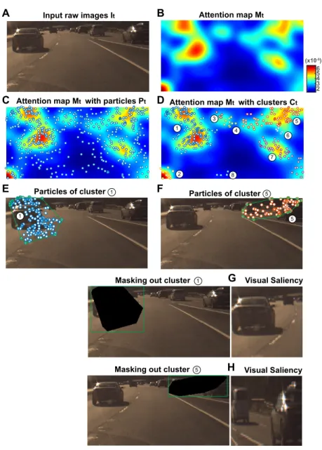
Gaussian filtering [12] as discussed in [88] (see Figure 3.2 (A,B)).

To extract a local visual saliency, we first randomly sample 2DN particles with

(34)

Input raw images It

Particles of cluster _{Particles of cluster}

Masking out cluster

Visual Saliency Visual Saliency Attention map Mt (x10-5₎ 2 3 4 5 6

Attention map Mt with particles Pt _{Attention map M}twith clusters Ct

1 2 3 4 5 6 7 8 5 1 1 1 5 5 A C E B D F G H

Figure 3.2: Overview of our fine-grained decoder. Given an input raw pixels It (A), we

compute an attention map Mt with a function fmap (B). (C) We randomly sample 3D

N = 500 particles over the attention map, and (D) we apply a density-based clustering

algorithm (DBSCAN [21]) to find a local visual saliency by grouping particles into clusters.

(E, F) For each cluster c∈ C, we compute a convex hullH(c) to define its region, and mask

out the visual saliency to see causal effects on prediction accuracy (see E, F for clusters 1 and 5, respectively). (G, H) Warped visual saliencies for clusters 1 and 5, respectively.

(35)

Algorithm 1: Fine-grained Decoder: Causality Check

Data: A consecutive set of {ut} and images {It} and

Result: A set of visual saliencies S

Get a set of {αt,i} and prediction errors {εt} by running Encoder and Decoder for

all images {It};

P ←φ, S ←φ;

for t = 0 toT-1 do

Get a 2D attention map Mt=fmap({αt,i});

Get a set Pt of randomly sampled 2D N points conditioned on Mt;

Aggregate datasets: P ←P ∪ {Pt, t};

end

Run clustering algorithm on P and get clusters {Ct};

for t = 0 toT-1 do

for each cluster c ∈ Ct do

Get a convex hull H(c);

Masking out pixels on H(c) from It;

Get a new prediction error ˆεt;

if |εˆt−εt|> δ then

Aggregate saliency S ← S ∪H(c);

end end end

time-axis as the third dimension to consider temporal features of visual saliencies. We thus

store spatio-temporal 3D particles P ← P ∪ {Pt, t}(see Figure 3.2 (C)).

We then apply a clustering algorithm to find a local visual saliency by grouping 3D

particlesP into clusters{C}(see Figure 3.2 (D)). In our experiment, we use DBSCAN [21], a

density-based clustering algorithm that has advantages to deal with a noisy dataset because they group particles together that are closely packed, while marking particles as outliers

that lie alone in low-density regions. For points of each cluster c and each time frame t,

we compute a convex hull H(c) to find a local region of each visual saliency detected (see

Figure 3.2 (E, F)).

For points of each cluster cand each time frame t, we iteratively measure a decrease of

prediction performance with an input image which we mask out a local visual saliency. We

compute a convex hull H(c) to find a local, and mask out each visual saliency by assigning

zero values for all pixels lying inside each convex hull. Each causal visual saliency is

gen-erated by warping into a fixed spatial resolution (=64×64) as shown in Figure 3.2 (G, H).

Algorithm 1 explains a pseudo-code for this step.

Feature-level Masking Approach. Along with devising the fine-grained decoder, we may consider using feature-level masking approach. Masking out convolutional features of

(36)

at-CHAPTER 3. INTERPRETABLE LEARNING FOR SELF-DRIVING CARS BY

tended region can provide a computationally efficient way by removing multiple forward passes of the convolutional network. This approach, however, may suffer from low decon-volutional spatial resolution, which makes challenge to view as a unit apart and divide the whole attention map into distinct attended objects, such as cars or lane markings.

3.3 Experiments

3.3.1 Datasets

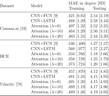
As explained in Table 3.1, we obtain two large-scale datasets that contain over 1,200,000

frames (≈16 hours) collected from Comma.ai [19], Udacity [78], and Hyundai Center of

Ex-cellence in Integrated Vehicle Safety Systems and Control (HCE) under a research contract. These three datasets acquired contain video clips captured by a single front-view camera mounted behind the windshield of the vehicle. Alongside the video data, a set of time-stamped sensor measurement is contained, such as vehicle’s velocity, acceleration, steering angle, GPS location and gyroscope angles. Thus, these datasets are ideal for self-driving studies. Note that, for sensor logs unsynced with the time-stamps of video data, we use the estimates of the interpolated measurements. Videos are mostly captured during highway driving in clear weather on daytime, and there included driving on other road types, such as residential roads (with and without lane markings), and contains the whole driver’s activities such as staying in a lane and switching lanes. Note also that, we exclude frames when the

vehicle stops which happens when ˆvt<1 m/s.

3.3.2 Training and Evaluation Details

To obtain a convolutional feature cube xt, we train the 5-layer CNNs explained in

Sec-tion 3.2.2 by using addiSec-tional 5-layer fully connected layers (i.e. # hidden variables: 1164,

100, 50, and 10, respectively), of which output predicts the measured inverse turning

ra-dius ut. Incidentally, instead of using addition fully-connected layers, we could also obtain

a convolutional feature cube xt by training from scratch with the whole network. In our

experiment, we obtain the 10×20×64-dimensional convolutional feature cube, which is then

flattened to 200×64 and is fed through the coarse-grained decoder. Other recent types of

more recent expressive networks may give a performance boost over our CNN configuration. However, exploration of other convolutional architectures would be out of our scope.

We experiment with various numbers of LSTM layers (1 to 5) of the soft deterministic visual attention model but did not observe any significant improvements in model perfor-mance. Unless otherwise stated, we use a single LSTM layer in this experiment. For training, we use Adam optimization algorithm [40] and also use dropout [73] of 0.5 at hidden state connections and Xavier initialization [23]. We randomly sample a mini-batch of size 128,

(37)

Dataset

Comma.ai [19] HCE Udacity [78]

# frame 522,434 80,180 650,690

FPS 20Hz 20Hz/30Hz 20Hz

Hours ≈ 7 hrs ≈ 1 hr ≈ 8 hrs

Condition Highway/Urban Highway Urban

Location CA, USA CA, USA CA, USA

Lighting Day/Night Day Day

Table 3.1: Dataset details. Over 16 hours (>1,200,000 video frames) of driving dataset

that contains a front-view video frames and corresponding time-stamped measurements of vehicle dynamics. The data is collected from two public data sources, Comma.ai [19] and Udacity [78], and Hyundai Center of Excellence in Vehicle Dynamic Systems and Control (HCE).

24 hours to train on a single NVIDIA Titan X Pascal GPU. Our implementation is based on Tensorflow [1] and code will be publicly available upon publication.

Two datasets (Comma.ai [19] and HCE) we used were available with images captured by a single front-view camera. This makes it hard to use the data augmentation technique

proposed by Bojarski et al. [9], which generated images with artificial shifts and rotations

by using two additional off-center images (left-view and right-view) captured by the same vehicle. Data augmentation may give a performance boost, but we report performance without data augmentation.

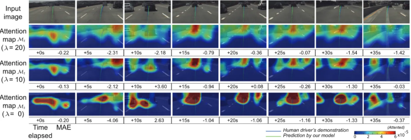
3.3.3 Effect of Choosing Penalty Coefficient

λ

Our model provides a better way to understand the rationale of the model’s decision by visualizing where and what the model sees to control a vehicle. Figure 3.3 shows a consecutive input raw images (with sampling period of 5 seconds) and their corresponding attention

maps (i.e. Mt =fmap({αt,i})). We also experiment with three different penalty coefficients

λ∈ {0,10,20}, where the model is encouraged to pay attention to wider parts of the image

(see differences between the bottom 3 rows in Figure 3.3 ) as we have larger λ. For better

visualization, an attention map is overlaid by an input raw image and color-coded; for example, red parts represent where the model pays attention. For quantitative analysis, prediction performance in terms of mean absolute error (MAE) is explained on the bottom of each figure. We observe that our model is indeed able to pay attention on road elements, such as lane markings, guardrails, and vehicles ahead, which is essential for human to drive.

Explainable and Advisable Learning for Self-driving Vehicles

UC Berkeley

UC Berkeley Electronic Theses and Dissertations

Contents

Acknowledgments

Chapter 1

Introduction

Chapter 2

Deep Traffic Light Detection for

Self-driving Cars from a Large-scale

Dataset

2.1

Problem Statement

RED

2.2

Deep Traffic Light Detection Model

2.2.1

Preprocessing

2.2.2

Coarse-grained Traffic Light Detection

2.2.3

Characterizing Traffic Lights

2.2.4

Spatiotemporal Filtering

2.3

Dataset

2.4

Experiments

2.4.1

Training and Evaluation Details

2.4.2

Quantitative Analysis

12,000

N

u

m

b

e

r

o

f

a

n

n

o

ta

ti

o

n

s

10,000

8,000

6,000

4,000

2,000

0

2.4.3

Real-world Experiments

A

B

Classes

without

Fine-grained detector

with

Fine-grained detector

Precision Recall F-measure Precision Recall F-measure

Red circle

70.20

29.70

41.74

68.00

29.50

41.15

Yellow circle

2.20

40.00

4.17

6.00

30.90

10.05