Fakult¨
at f¨
ur Informatik
Lehrstuhl f¨
ur Bildverarbeitung und K¨
unstliche Intelligenz
Efficient Large-Scale Stereo
Reconstruction using Variational
Methods
Georg Kuschk
Vollst¨andiger Abdruck der von der Fakult¨at f¨ur Informatik der Technischen Universit¨at M¨unchen zur Erlangung des akademischen Grades eines
Doktors der Naturwissenschaften (Dr. rer. nat.)
genehmigten Dissertation.
Vorsitzender: Prof.Dr.-Ing.MatthiasNießner Pr¨ufer der Dissertation: 1. Prof. Dr. Daniel Cremers
2. Prof. Dr. Michael M¨oller Universit¨at Siegen
Die Dissertation wurde am 31.10.2018 bei der Technischen Universit¨at M¨unchen eingereicht und durch die Fakult¨at f¨ur Informatik am 13.03.2019 angenommen.
This thesis investigates the use of convex variational methods for depth reconstruc-tion from optical imagery and fusion of multiple depth maps into combined depth maps with higher accuracy. Dense depth reconstruction from two or more camera views are an important subject of research in computer vision, since measurement density is much higher than other depth sensing techniques, namely active depth sensing via infrared pattern projection or Lidar and Radar based techniques - even though the latter ones are more accurate and robust in depth. Other advantages of cameras are their low costs and low power consumption due to their passive sensing principle. Approaches are ranging from autonomous driving cars, obstacle avoid-ance or surveying UAVs up to detailed reconstruction of remote terrains using space borne imagery.
In particular, we propose a fast algorithm for high-accuracy large-scale outdoor dense stereo reconstruction. To this end, we present a structure-adaptive second-order To-tal Generalized Variation (TGV) regularization which facilitates the emergence of planar structures by enhancing the discontinuities along building facades. Instead of solving the arising optimization problem by a coarse-to-fine approach, we pro-pose a quadratic relaxation approach which is solved by an augmented Lagrangian method. This technique allows for capturing large displacements and fine structures simultaneously.
For the application in autonomous driving, we further present an algorithm for dense and direct large-scale visual SLAM that runs in real-time on a commodity notebook. We developed a fast variational dense 3D reconstruction algorithm which robustly integrates data terms from multiple images thus enhancing quality of the image matching. An additional property of this variational reconstruction framework is the ability to integrate sparse depth priors (e.g. from RGB-D sensors or LiDAR data) into the early stages of the visual depth reconstruction, leading to an implicit sensor fusion scheme for a variable number of heterogenous depth sensors. Em-bedded into a keyframe-based SLAM framework, this results in a memory efficient representation of the scene and therefore (in combination with loop-closure detec-tion and pose tracking via direct image alignment) enables us to densely reconstruct large scenes in real-time.
Finally, applied to space-borne remote sensing, we present an algorithm for robustly fusing digital surface models (DSM) with different ground sampling distances and confidences, using explicit surface priors to obtain locally smooth surface models. The optimization using L1 based differences between the separate DSMs and
in-corporating local smoothness constraints is also inherently able to include weights for the input data, therefore allowing to easily integrate invalid areas, fuse multi-resolution DSMs and to weigh the input data.
Diese Arbeit untersucht die Verwendung von konvexen Variationsmethoden f¨ur die Tiefenrekonstruktion anhand optischer Bilder und die Fusion mehrerer Tiefenkarten in kombinierte Tiefenkarten mit h¨oherer Genauigkeit. Eine dichte Tiefenrekonstruk-tion aus zwei oder mehr Kameraansichten ist ein wichtiges Thema der Computer-bildverarbeitung, da die Messdichte viel h¨oher ist als bei anderen Tiefenmesstech-niken, insbesondere aktiven Tiefenmessungen mittels Infrarotmusterprojektion oder Lidar- und Radar-basierte Techniken - auch wenn diese genauer und robuster in der Tiefenmessung sind. Weitere Vorteile von Kameras sind ihre geringen Kosten und ihr geringer Stromverbrauch aufgrund ihres passiven Messprinzips. Die Ans¨atze rei-chen von autonom fahrenden Autos ¨uber die Vermeidung von Hindernissen oder die Vermessung durch UAVs bis hin zur detaillierten Rekonstruktionen von abgelegenen Gebieten mit Hilfe von weltraumgest¨utzten Bildaufnahmen.
Insbesondere schlagen wir einen schnellen Algorithmus f¨ur eine hochgenaue, dichte Stereo-Rekonstruktion f¨ur großr¨aume Outdoor-Szenarien vor. Zu diesem Zweck pr¨asentieren wir eine strukturadaptive TGV-Regularisierung (Total Generalized Variation) zweiter Ordnung, welche die Entstehung planarer Strukturen durch die Verbesserung der Diskontinuit¨aten entlang von Geb¨audefassaden erleichtert. Anstatt das entstehende Optimierungsproblem durch einen Coarse-to-Fine-Ansatz zu l¨osen, schlagen wir einen quadratischen Relaxationsansatz vor, der durch eine Augmented Lagrange Methode gel¨ost wird. Mit dieser Technik k¨onnen große Ver-schiebungen naher Objekte im Bildbereich wie auch feine Strukturen gleichzeitig erfasst werden.
F¨ur die Anwendung im autonomen Fahren stellen wir außerdem einen Algorith-mus f¨ur dense und direct large-scale visual SLAM vor, das in Echtzeit auf einem Standard-Notebook l¨auft. Wir haben einen effizienten, variationsbasierten dichten 3D-Rekonstruktionsalgorithmus entwickelt, der Daten aus mehreren Bildern robust integriert und somit die Qualit¨at des Bildmatchings verbessert. Eine zus¨atzliche Eigenschaft dieses variationsbasierten Rekonstruktionsframeworks ist die F¨ahigkeit, d¨unnbesetzte Tiefen a-priori Informationen (z.B. von RGB-D-Sensoren oder LiDAR-Daten) in die fr¨uhen Stadien der Rekonstruktion der visuellen Tiefe zu integrieren, was zu einem impliziten Sensorfusionsschema f¨ur eine variable Anzahl heterogener Tiefensensoren f¨uhrt. Eingebettet in ein Keyframe-basiertes SLAM-Framework f¨uhrt dies zu einer speichereffizienten Darstellung der Szene und erm¨oglicht somit (in Kombination mit Loop-Closure-Erkennung und Pose-Tracking ¨uber direct image alignment) die dichte Rekonstruktion von umfangreichen Szenen in Echtzeit.
Schließlich stellen wir einen Algorithmus zur robusten Fusionierung von digitalen Oberfl¨achenmodellen (DSM) mit verschiedenen Bodenabtastungsabst¨anden und Konfidenzen vor, wobei explizite Oberfl¨achen priors verwendet werden, um lokal glatte Oberfl¨achenmodelle zu erhalten. Die Optimierung unter Verwendung von auf der L1-Norm basierenden Differenzen zwischen den einzelnen DSMs und dem
Ein-beziehen lokaler Glattheitseinschr¨ankungen ist auch inh¨arent in der Lage, Gewich-tungen f¨ur die Eingabedaten einzuschließen, wodurch es auch m¨oglich ist, ung¨ultige Bereiche ohne vorliegende Messpunkte in den Optimierungsprozess zu integrieren, DSMs mit mehreren verschiedenen Bodenabtastungsabst¨anden zu fusionieren und die Eingabedaten allgemein zu gewichten.
First of all, I would like to thank my doctoral advisor Prof. Daniel Cremers for giving me the opportunity to pursue my academic research under his supervision. My second referee Michael M¨oller deserves just as much appreciation. Both Daniel and Michael inspired and helped me a lot with excellent and fruitful discussions. During my time at the German Aerospace Center (DLR) I worked with many great people who also deserve huge credit. Namely I want to thank my colleagues and co-authors Pablo d’Angelo, Peter Reinartz, Thomas Krauss as well as my colleagues Peter Fischer, Oliver Meynberg, Ke Zhu, Jiaojiao Tian and my students Grigory Shelekov, Marina Schicht, Ksenia Davydova, David Gaudrie.
During my short time at the university of Graz (TUG) I was honored to make the acquaintance with Thomas Pock, whose inspirational sessions at the whiteboard were marvelous. Many thanks also go to Gottfried Graber and Ren´e Ranftl from whom I learned a lot of practical implementation details and tricks.
I also would like to thank all of my colleagues, co-authors, contributors and friends at the Technical University of Munich (TUM): Mohamed Souiai, Frank Steinbr¨ucker, Thomas M¨ollenhoff, Jan St¨uhmer, Robert Maier, Thomas Windheuser and my stu-dents during that time, all of them pursuing an interesting career now: Aljaz Bozic, Bj¨orn H¨afner and Dennis Mack.
Finally and foremost, many thanks got to my family for raising and supporting me as well as encouraging me all the time to follow my passion regardless the obstacles.
List of Figures xiii
List of Tables xv
1 Introduction 1
1.1 Motivation . . . 2
1.1.1 Remote sensing data . . . 4
1.1.2 Automotive data . . . 6
1.2 Literature Overview . . . 7
1.2.1 Datasets . . . 7
1.2.2 Stereo depth estimation . . . 7
1.2.3 Regularization . . . 9
1.3 Contributions of this Thesis . . . 11
1.3.1 Own Publications . . . 12
1.3.2 Thesis Outline . . . 14
2 Total Variation based Dense Stereo 15 2.1 Mathematical Preliminaries . . . 15
2.1.1 Notation . . . 15
2.1.2 Camera models . . . 17
2.2 Image Matching Cost Functions . . . 22
2.2.1 Normalized Cross Correlation . . . 24
2.2.2 Modified Census Transform . . . 24
2.2.3 Mutual Information . . . 25
2.2.4 Adaptive Support Weights . . . 26
2.2.5 Shortcomings . . . 27
2.3 Total Variation Regularization . . . 30
2.3.1 Total Variation . . . 30
2.3.2 Depth map denoising example . . . 32
2.4 Optimization . . . 39
2.4.1 Primal-Dual Algorithm . . . 39
2.4.2 Legendre-Fenchel Transformation . . . 40
2.4.3 f(x) = kxkδ . . . 42
2.4.5 Implementation details . . . 44
3 ADMM 47 3.1 Summary . . . 47
3.2 Introduction . . . 48
3.3 Edge-segment based adaptive regularization . . . 50
3.4 Fast optimization by quadratic splitting and augmented Lagrangian . 51 3.4.1 Convex solution . . . 51
3.4.2 Non-convex solution . . . 53
3.4.3 Augmented Lagrangian update . . . 53
3.5 Algorithm . . . 53
3.6 Evaluation . . . 56
3.7 Conclusion . . . 61
4 Dense SLAM 63 4.1 Summary . . . 63
4.2 Introduction and Related Work . . . 64
4.2.1 Related Work . . . 64
4.2.2 Contributions and Overview . . . 66
4.3 Dense Depth Reconstruction . . . 67
4.3.1 Multi-View Data Terms and Sparse Priors . . . 67
4.3.2 Optimization . . . 70
4.3.3 Reconstruction of Image Sequences . . . 74
4.4 Large-Scale Dense SLAM . . . 75
4.5 Results . . . 76
4.5.1 SLAM - KITTI Odometry Benchmark . . . 76
4.5.2 Sparse Priors . . . 77
4.5.3 Qualitative Results . . . 78
4.6 Conclusions . . . 79
5 Depth Map Fusion 81 5.1 Summary . . . 81 5.2 Introduction . . . 82 5.3 Method . . . 84 5.3.1 TV-L1 Fusion . . . 85 5.3.2 TGV-L1 Fusion . . . 85 5.3.3 Weighted TGV-L1 Fusion . . . 86 5.3.4 Parameters . . . 86 5.4 Optimization . . . 87 5.4.1 Implementation Details . . . 89 5.5 Evaluation . . . 91 5.5.1 Artificial Tests . . . 91
5.5.2 Artificial Tests - Weights . . . 91 5.5.3 Artificial Tests - Varying DSM resolution / Sparse DSM . . . 93 5.5.4 Unimodal DSM fusion . . . 93 5.5.5 Multimodal DSM fusion . . . 97 5.6 Conclusion . . . 103 6 Conclusion 105 6.1 Summary . . . 105 6.2 Future Work . . . 107 Bibliography 109
1.1 Large-scale 3D reconstruction of a complete SLAM framework . . . 2
1.2 Satellite based 3D reconstruction . . . 3
1.3 Overview of some common commercial optical satellites . . . 4
1.4 Exemplary Worldview-2 satellite imagery . . . 5
1.5 Exemplary imagery and Lidar data for urban driving scenarios . . . 6
1.6 Exemplary data from the Middlebury dataset . . . 8
2.1 2-view stereo problem with computed depth map . . . 16
2.2 Illustration of a Cost volume . . . 16
2.3 Reconstruction quality without and with regularizers . . . 17
2.4 Pinhole camera model . . . 18
2.5 Push broom camera model . . . 20
2.6 Trilinear interpolation of a camera model using a sparse lookup table . . 22
2.7 Trilinear interpolation . . . 22
2.8 Image matching cost functions with spatial support window . . . 23
2.9 Displacement field for census transform . . . 25
2.10 Basic scheme for adaptive support-weights . . . 26
2.11 Visualization of adaptive support-weights . . . 27
2.12 Examples of image regions ill-suited for image matching . . . 28
2.13 Image matching cost functions for selected points . . . 29
2.14 Staircasing effect of Total Variation . . . 34
2.15 Huber loss . . . 34
2.16 Impact of different regularization energy functionals . . . 36
2.17 Impact of different regularization energy functionals . . . 37
2.18 Impact of different regularization energy functionals . . . 38
2.19 Supporting hyperplanes of a closed convex set . . . 41
2.20 Examples for proximal mapping . . . 43
3.1 Detailed stereo reconstruction . . . 48
3.2 Influence of high-level edge priors on the anisotropic regularization . . . . 52
3.3 Subdisparity accurate results . . . 55
3.4 Evolution of the primal energy . . . 56
3.5 Results of the proposed algorithm for the Middlebury Stereo benchmark 57 3.6 Example results for the KITTI stereo benchmark . . . 58
4.1 Dense large-scale reconstruction for an automotive image sequence . . . . 64 4.2 Reconstruction results using different number of images . . . 68 4.3 Strengthening the image matching data term using multiple input images 69 4.4 Influence of adding sparse laser priors early in the 3D reconstruction . . 69 4.5 Workflow of 3D reconstruction from a successive image sequence . . . 75 4.6 Flowchart of the corresponding SLAM system . . . 75 4.7 Reconstruction results on Middlebury data simulating sparse depth priors 77 4.8 Dense large-scale reconstruction using automotive image data . . . 78 5.1 Four co-registered DSMs, obtained from optical stereo reconstruction . . 83 5.2 Comparison of local fusion method versus global optimization methods . 92 5.3 SNR values with varyingλd to obtain best parameter . . . 93
5.4 Evaluation of using explicit weights . . . 94 5.5 Evaluation of fusing DSMs with different ground sampling distance . . . 95 5.6 Exemplary optical images for evaluation of real-world satellite data . . . 98 5.7 London dataset: medmean, TV-L1 and TGV-L1 fusion for inner city . . 99
5.8 London dataset: medmean and TV-L1 fusion with error to ground truth 99
5.9 London dataset inner city: Fusion results . . . 100 5.10 ISPRS dataset: Exemplary WorldView-1 images . . . 101
1.1 Basic data of most common operational commercial optical satellites . . 5
1.2 Most commonly used datasets for evaluation of depth reconstruction . . 7
1.3 Peer-reviewed publications . . . 13
3.1 Results of the proposed algorithm for the Middlebury Stereo benchmark 57 3.2 Results for the challenging KITTI stereo benchmark . . . 58
4.1 Averaged timings per frame . . . 77
5.1 Las Vegas dataset: Accuracy of the fused DSM . . . 96
5.2 London dataset (Inner City): Accuracy of the fused DSM . . . 96
5.3 London dataset (Park): Accuracy of the fused DSM . . . 96
Chapter
1
Introduction
With advancing automation, large-scale 3D reconstruction is increasingly becoming more important in various scientific fields as well as in common life. Applications are ranging from autonomous driving of cars or mobile robots in general, flight planning for unmanned aerial vehicles or remote sensing based digital surface re-construction for wide-area physical simulations like flood simulation, propagation of radio beams, 3D change detection etc. Despite the advances of modern active
depth-sensing technologies like Lidar, Radar, Time-of-Flight and projector-camera systems, depth estimation based on cameras only still is on par with these active sensing technologies.
The advantages of a very high spatial resolution, dense measurements, the absence of interferencing problems due to passive sensing, cheap costs and low power consump-tion render cameras as a very attractive sensor for this problem. From a philosoph-ical point of view, one could even argue, that most higher biologphilosoph-ical life uses optphilosoph-ical systems for navigation, thereby implying that evolution proved this a good choice for environmental sensing. Camera-only systems of course have their own short com-ings for 3D reconstruction (aperture problem / repetitive textures, textureless image regions, specular reflections, semi transparent surfaces etc). This directly implies a smart combination and fusion of different sensor modalities, thereby mitigating their respective shortcomings, in cases where this is applicable.
So despite being an active research area for decades, the need for more accurate and robust results as well as computationally cheap approaches still drives investigation in the field of optical 3D reconstruction. In this work the aspect of obtaining very fast dense depth reconstruction, while simultaneously achieving high accuracy, is being investigated. Apart from the reconstruction process itself, fusing image- and depth information from multiple images is examined as well. This work attempts to meet the demands of two somewhat different applications:
• Far-range satellite based depth reconstruction.
While the automotive application has very strict real-time requirements and operates on images the size of 106 −107 pixel, captured with 10-30 frames per second, the remote sensing application typically consists of only 1-3 captured images of the scene, with a size of roughly 109 pixel per image.
For the automotive scenario, this results in very short inter-frame distances, both temporarily and spatially, making this use case applicable for fusing different depth maps to a single depth map exhibiting higher accuracy. Due to the short baseline between captured images, perspective changes only slightly between images, thereby simplifying the problem of matching image areas between two frames.
For remote sensing imagery arising from satellites or aerial sensors, the baseline between two captured images is typically very large (15 - 60◦), resulting in quite different reflection properties of the captured surfaces.
Motivation
As a practical motivation Figure 1.1 shows an application of large scale 3D re-construction based on close-range sensing mobile cameras, e.g. in the case of au-tonomous driving. In these scenarios, where thousands of successive depth maps are generated with the mobile platform dynamically moving around the scene, im-portant aspects like drifting position estimation (compared to ground truth) and revisiting of identical places have to be considered by applying an overall SLAM framework. We will discuss this in detail in Chapter 4.
Different sensor technologies exist, nowadays namely Lidar sensors, which have a higher longitudinal accuracy, but suffer from sparsity and missing texture informa-tion. Also in Chapter 4 we propose a strategy for depth estimation from camera with the optional help of integration existing sparse depth data early in the reconstruction process.
Figure 1.1: Resulting large scale 3D reconstruction of a complete SLAM framework in automotive driving scenarios - as will be described in Chapter 4.
Figure 1.2 gives an overview of remote sensing based surface reconstruction and some exemplary applications. While radar satellites - based on Synthetic Aperture Radar (SAR) like TanDEM-X and TerraSAR-X do not suffer from clouds occluding the observed surface and exhibiting high longitudinal accuracy, their lateral resolu-tion and accuracy is very low compared to optical satellites and of course surface texture cannot be captured as well. An obvious approach would be fusing the corre-sponding 3D information while retaining the advantageous properties of each input data. In Chapter 5 we will have a detailed look at how to accomplish this fusion.
(a) 3D reconstruction for autonomous flight planning
(b) Space-borne 3D reconstruction
Figure 1.2: Satellite based 3D reconstruction, serving exemplary applications like change detection in restricted areas or unchartered, sprawling mega cities, like flood simulations, propagation of radio beams, autonomous flight planning etc.
Remote sensing data
As spaceborne remote sensing data is not readily available for most computer vision researchers, we would like to give a short introduction over the nature of correspond-ing satellite data. A detailed explanation of the image capturcorrespond-ing process and the camera model is given in Section 2.1.2.
(a) Worldview satellites, image credit https://www. digitalglobe.com
(b) One of the Pleiades satellites, im-age credit https://pleiades.cnes. fr
Figure 1.3: Overview of some common commercial optical satellites. Each satellite produces data of approximately 1 terabyte per day with images having a size of around 1 gigapixel and a ground sampling distance (GSD) of 0.3-0.8m.
Even though the main use case is 2D monitoring of land surfaces, the already captured image data can be readily used for 3D reconstruction processes. However, due to the altitude of roughly 700km to the observed surface, it is practically not possible to capture images with a satellite mounted stereo camera from one spe-cific position in orbit and perform 3D reconstruction on these. Instead - to get a convenient baseline for the underlying triangulation process - images from different position (and therefore different time steps) are used. Since the 3D reconstruction process typically involves a static world assumption, this leads to problems with large moving objects as can be seen in Figure 1.4.
Geolocation accuracy (= pose estimation) of the satellites is typically in the range of 3m, if ground control points (known reference points in the image) are given accu-racy is in range of 1m. Pose estimation of satellites is done using a start tracker as an optical device to identify and measure the position of given stars and inertial mea-surement units (IMU) consisting of gyroscopes and accelerometers. Life expectancy (based on decommissioned satellite like IKONOS and Quickbird) is typically in the range of 7-13 years.
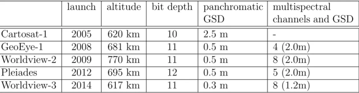
launch altitude bit depth panchromatic GSD multispectral channels and GSD Cartosat-1 2005 620 km 10 2.5 m -GeoEye-1 2008 681 km 11 0.5 m 4 (2.0m) Worldview-2 2009 770 km 11 0.5 m 8 (2.0m) Pleiades 2012 695 km 12 0.5 m 5 (2.0m) Worldview-3 2014 617 km 11 0.3 m 8 (1.2m)
Table 1.1: Basic data of most common operational commercial optical satellites
(a) Satellite position at time stept (b) Satellite position at time stept+ 1
Figure 1.4: Exemplary Worldview-2 satellite imagery. Please note the strong perspective change between consecutive images (slanted buildings) and temporal (moving boats) change, as well as large occlusion areas between the skyscrapers. Despite a bit depth of 11 Bit the shadows have a very low signal-to-noise ratio.
Automotive data
For the application of depth sensing in highly-automated driving scenarios, we use the well-known and publicly available KITTI data [34], which for our tasks consists of two automotive stereo camera systems (RGB and gray) and a 64-layer laser scanner. See Figure 1.5 for exemplary data.
(a) Left camera frame
(b) 3D Lidar data projected into 2D image space
(c) Dense depth reconstruction
Figure 1.5: Exemplary imagery and Lidar data for urban driving scenarios as in [34], plus dense depth reconstruction as described in Chapter 4
Literature Overview
Datasets
Despite earlier research, the publication of the Middlebury Stereo Benchmark [99], [100] marked a milestone in the development of depth reconstruction algorithms, allowing evaluation and comparison of the evolving ideas and algorithms on a stan-dardized benchmark instead of judging the quality on non-public and withheld data. Over the next years, with continuously improving reconstruction quality the dataset was extended multiple times to incorporate more challenging data [48] and [98] (see Figure 1.6). Still the acquired data covered only indoor scenarios due to the ground truth depth acquisition system based on structured light and continued being re-stricted to 2-view stereo imagery.
As a logical extension, and with the advent of more and more automotive scenarios in industry, real-world outdoor datasets like the famous KITTI dataset were pub-lished [34], [71], [54], covering challenging outdoor scenarios as well. As of now, the corresponding ground truth is generated using a calibrated and synchronized laser scanning system.
With the upcoming success of deep learning approaches, the need for training data grew exponentially, thus training data generation became very expensive. This lead to the generation of various synthetic datasets, such as [16], [68], [118], [95], [94].
Stereo depth estimation
An overview of the most commonly used datasets for evaluation of depth reconstruc-tion is given in Table 1.2. The number of submissions indicates a vivid development and active research in this field, making a complete overview of depth reconstruction algorithms intractable in this chapter. We rather give a short overview of a group of algorithms which dominated the field of depth reconstruction by their respective time.
Dataset Number of submissions in benchmark
Middlebury 2003 [100] 167
Middlebury 2014 [98] 71
KITTI 2012 [34] 100
KITTI 2015 [71] 84
Table 1.2: Most commonly used datasets for evaluation of depth reconstruction
Finding the best-matching image patch in other images for a given pixel position in a reference image, together with the corresponding camera positions, allows for
(a) Input image (b) Ground truth (color coded depth)
(c) Input image (d) Ground truth (color coded depth) Figure 1.6: Exemplary data from the Middlebury dataset [98]
triangulation and therefore estimating the depth of that particular pixel. In Section 2.1 and 2.1.2 we will go further into detail, but we will highlight the state of the art of image matching cost functions in this section.
Due to perspective changes, illumination changes, occlusions etc, image matching itself is not trivially leading to the optimal solution and much research was done investigating proper image matching cost functions. Very simple cost functions with no spatial support are for example AD (absolute difference), Birchfield-Tomasi mea-sure [8] or Mutual Information [116].
Comparing the intensity values of two corresponding pixels alone is prone to noise and ambiguities (see Figure 2.13) and therefore more local image information needs to be incorporated into the image matching cost functions. The two opposing prin-ciples which must be met are a large spatial support for generating descriptive and discriminative features vectors on the one hand and a small spatial support on the other hand, as spatial support implies assumptions of the depth of neighboring pix-els, leading to local planarity assumption.
To restrict computational complexity, fronto-parallel assumption of the neighboring pixels (all 3D points lying on a plane parallel to the image plane) is the standard case resulting in cost functions comparing image patches around the pixel position using sum of absolute difference (SAD), sum of squared differences (SSD), normal-ized cross correlation (NCC), Census transform [125] etc. For high accuracy cases, evaluating the cost function on multiple (slanted) planes is possible as well [33], [10]. The aforementioned Census transform is a very powerful image descriptor for dense image matching because it is robust to many forms of illumination changes (to some degree even non-linear ones such as specularities) and at the same time com-putationally very cheap. Naturally. different work was done trying to improve the descriptive and discriminative strength while at the same time maintaining the speed. Replacing the binary comparison with a ternary decision was done in [105], increasing robustness against noise, especially at the central pixel. In [32] intensities are not compared with the central pixel intensity directly but with the mean value of its 3×3 neighborhood, also increasing robustness against noise. A scale-robust Census matching was introduced in [88], based on a circular sampling strategy with different radii corresponding to different scales and taking the minimum cost over these different scales.
A common approach to further strengthen the image matching cost function is lo-cal cost aggregation based on pixel similarities in terms of color and distance as described in the seminal work of Adaptive support-weights [124] which will be also described in detail in Section 2.2.
Of the advanced and more descriptive features (mainly used in image recognition) like SIFT [67], SURF [2], BRIEF [17], BRISK [64] only the DAISY descriptor [114], designed for speed, showed a somewhat acceptable speed for using it in dense stereo reconstruction. Due to some invariance against rotation, scaling and simple radio-metric changes, using the DAISY descriptors (or any other of the abovementiond features) yields very good results for wide-baseline stereo like in satellite based 3D reconstruction, where some simple dissimilarity measures fail because of the large perspective differences.
For more detailed evaluations of different cost functions, we refer to the surveys of e.g. [99], [112], [48], [49].
Regularization
Despite much work on the image matching cost functions, estimation of the depth of a pixel is still largely independent of its neighboring pixels, leading to noisy cost functions and wrong depth estimation due to local minima (see Figure 2.13 and 2.3). To reduce noise in the resulting depth map a very simple approach is to run a 2D median filtering on the depth map, replacing outliers by the median depth in a local support window. This approach however only partly cures the symptoms on much reduced data - instead of addressing the original problem earlier with all input data
(information about the image matching cost functions especially) still available. To this end, instead of estimating the depth of each pixel solely on its image match-ing information, additional priors on the resultmatch-ing 3D surfaces are enforced in the overall reconstruction process as described in detail in Section 2.1. These priors are typically called smoothness terms, referring to the effect of favoring locally planar surfaces in the 3D reconstruction. To do so, they enforce pixels in a local neigh-borhood to have similar values for depth. However, computing the optimal solution of such a reconstruction problem becomes in general extremely hard because of the implied computational demand and combinatorial complexity. Thus, many approxi-mation techniques have been investigated, with the goal of having a guaranteed local optimum close to the global one while being as fast as possible. A detailed overview of the results of the past two decades of research spent in this field is out of scope of this thesis. So we limit ourselves to a short overview of a group of algorithms which dominated the field of depth reconstruction by their respective time.
Markov Random Fields[13], [50], [12], [53] and Belief Propagation [111], [123], [122] were the first family of such algorithms, dominating the state-of-the-art at their time and in simple special cases even guaranteeing to result in a global optimum. The basic idea of Markov Random Fields is posing the depth reconstruction (and other image processing tasks) as labeling problem, assigning each pixel a label cor-responding to its depth, while at the same time taking into account the interaction between neighboring pixels, namely enforcing similar labels in a local neighborhood. While this labeling from a combinatorial point of view is NP-hard, the seminal paper of [13] framed the problem as a specialized graph for the energy function which then can be approximately minimized via repeatedly applying efficient max-flow min-cut algorithms. An overview of such max-flow min-cut algorithms can be found in [9].
Semi Global Matching (SGM) was developed shortly afterwards in the work of [44], [45], [48], [46],[49], [47]. Instead of tackling the hard 2-dimensional problem, this remarkably efficient family of algorithms is iteratively passing over the image in 1-dimensional sweeps from different directions and solving the separate 1D problems via efficient and accurate dynamic programming. The result after each such direc-tional scan is passed as approximate solution to the next direcdirec-tional pass where it is again refined. SGM might not be the most accurate algorithm, but because of it’s low computational complexity it is widely used for real-time depth reconstruction on low-cost hardware.
Variational Methodswere brought to interest by the seminal paper of Rudin, Osher and Fatemi [96], who introduced total variation for image denoising. Similar to Markov Random Fields, minimizing the total variation of a functional defined over image space is done iteratively, with a spatially limited direct interaction of variables. Instead of enforcing smooth discrete depth-labels to neighboring pixels, variational methods inherently minimize on a continuous label space by solving the differential equations arising from minimizing the first order derivative of the depth
map (minimizing jumps in depth between neighboring pixels). With the advent of modern general purpose graphics processing units (GPGPU or just GPU), these highly parallelizable algorithms became computationally feasible, thereby boosting research in this field [19],[21], [84], [83], [85] culminating in the celebrated paper introducing the primal-dual algorithm [22].
Providing a general framework and an efficient solution including convergence guar-antees for a large number of optimization problems, this work is also the underlying foundation of this thesis. For a very detailed overview of applying Total Variation for image analysis we refer to the well written report of [20]. In a follow-up work [82] the primal-dual algorithm was further accelerated by using local step-sizes for the gradient descent based optimization steps instead of the former global step size. Although the primal-dual algorithm is applicable to a large number of optimization problems, it was already used for depth reconstruction in the original paper [22], with a large number of follow-up work like [36], [89], [90].
The original work contained a regularization term for the depth reconstruction by directly minimizing the sum of gradients of the resulting depth map, thereby favor-ing fronto-parallel surfaces. In [14] and [87] this constraint was lifted and extended to higher order regularizers by the so-called Total Generalized Variation (TGV). Es-pecially for depth reconstruction the 2nd order TGV has a major impact by favoring slanted locally planar surfaces in the scene.
An anisotropic version of the regularizers based on the Nagel-Enkelmann operator [74] was further introduced and used for TV [120] as well as for TGV [89]. Tackling the problem of over-smoothing image areas with large depth changes, the smooth-ing amount could now be steered accordsmooth-ing to additional image cues (like e.g. edge information).
In [119] and [88] the Markov property of image pixels only interacting directly with their direct adjacent neighbors was relaxed by allowing direct interactions over fur-ther distances (Non-Local Total Variation). As a downside of this, memory con-sumption increases and convergence speed drops significantly.
Aside from the depth reconstruction application, variational approaches can also readily be applied to denoising and fusing multiple low-quality depth maps which will be detailed in Section 5, building up or having similarity to the work of [127], [126], [87], [30], [80].
Contributions of this Thesis
This thesis focuses and summarizes the work presented in [59], [58], [?], which is the result of the joint work with Pablo d’Angelo, David Gaudrie, Aljaˇz Boˇziˇc, Prof. Peter Reinartz and Prof. Daniel Cremers. Closely related work was additionally presented in [56], [57], [60] and a complete list of all publications published throughout the period of this thesis is given in Table 1.3. All included papers
are peer-reviewed publications and were published in international conferences or journals.
In chapter 3, we propose a fast algorithm for high-accuracy large-scale out-door dense stereo reconstruction. To this end, we present a structure-adaptive second-order Total Generalized Variation (TGV) regularization which facilitates the emergence of planar structures by enhancing the discontinuities along building facades. Instead of solving the arising optimization problem by a coarse-to-fine approach, we propose a quadratic relaxation approach which is solved by an augmented Lagrangian method. This technique allows for capturing large displace-ments and fine structures simultaneously.
For the application in autonomous driving, we further present an algorithm for dense and direct large-scale visual SLAM in Chapter 4 that runs in real-time on a commodity notebook. We developed a fast variational dense 3D recon-struction algorithm which robustly integrates data terms from multiple images thus enhancing quality of the image matching. An additional property of this variational reconstruction framework is the ability to integrate sparse depth priors (e.g. from RGB-D sensors or LiDAR data) into the early stages of the visual depth reconstruction, leading to an implicit sensor fusion scheme for a variable number of heterogenous depth sensors. Embedded into a keyframe-based SLAM framework, this results in a memory efficient representation of the scene and therefore (in combination with loop-closure detection and pose tracking via direct image alignment) enables us to densely reconstruct large scenes in real-time.
In Chapter 5, applied to space-borne remote sensing, we present an algorithm for robustly fusing digital surface models (DSM) with different ground sampling dis-tances and confidences, using explicit surface priors to obtain locally smooth surface models. The optimization using L1 based differences between the separate DSMs
and incorporating local smoothness constraints is also inherently able to include weights for the input data, therefore allowing to easily integrate invalid areas, fuse multi-resolution DSMs and to weight the input data.
Authors Title Publication medium [58] Kuschket al. Real-time Variational Stereo
Re-construction with Applications to Large-scale Dense SLAM
IEEE Intelligent Vehicles Symposium, 2017
[61] Kuschket al. Spatially Regularized Fusion of Multiresolution Digital Surface Models
IEEE Transactions on Geo-science and Remote Sensing, 2017
[26] Davydovaet al. Consistent Multi-View Texturing of Detailed 3D Surface Models
ISPRS Annals of the Pho-togrammetry Remote Sensing and Spatial Information Sci-ences, 2015
[55] Krausset al. 3D-Information Fusion from Very High Resolution Satellite Sensors
Proceedings of International Symposium on Remote Sens-ing of Environment (ISRSE), 2015
[62] Kuschket al. DSM Accuracy Evaluation for the ISPRS Commission I Image Matching Benchmark
ISPRS - International Archives of the Photogram-metry, Remote Sensing and Spatial Information Sciences, 2014
[25] d’Angeloet al. Evaluation of Skybox Video and Still Image Products
ISPRS - International Archives of the Photogram-metry, Remote Sensing and Spatial Information Sciences, 2014
[93] Reinartzet al. Advances in DSM Generation and Higher Level Information Extrac-tion from High ResoluExtrac-tion Optical Stereo Satellite Data
European Association of Re-mote Sensing Laboratories (EARSeL), 2014
[59] Kuschket al. Fast and Accurate Large-scale Stereo Reconstruction using Vari-ational Methods
ICCV Workshop on Big Data in 3D Computer Vision, 2013 [57] Kuschket al. Model-Free Dense Stereo
Recon-struction for Creating Realistic 3D City Models
Joint Urban Remote Sensing Event (JURSE), 2013 [56] Kuschket al. Large Scale Urban Reconstruction
from Remote Sensing Imagery
International Archives of the Photogrammetry, Remote Sensing and Spatial Infor-mation Sciences (ISPRS), 2013
[72] Meynberget al. Airborne Crowd Density Estima-tion
ISPRS Annals of the Pho-togrammetry, Remote Sens-ing and Spatial Information Sciences, 2013
[60] Kuschket al. Fusion of Multi-Resolution Digital Surface Models
ISPRS - International Archives of the Photogram-metry, Remote Sensing and Spatial Information Sciences, 2013
[24] d’Angeloet al. Dense Multi-View Stereo from Satellite Imagery
IEEE International Geo-science and Remote Sensing Symposium (IGARSS), 2012
Thesis Outline
This cumulative thesis is structured into six chapters.
In Chapter 1 we give an introduction and motivation of this thesis, providing an overview of relevant literature, as well as giving an overview of the research papers that were published during this thesis.
Chapter 2 presents an overview of the mathematical background in general, de-scribes the involved camera models, stereo image matching functions and regular-ization techniques as well as a general framework for numerical optimregular-ization of the developed models.
In Chapter 3, 4 and 5 we present our work of [59], [58], [?] respectively in detail. We conclude this thesis with Chapter 6, summarizing our research and giving an outlook towards future research possibilities.
Chapter
2
Total Variation based Dense
Stereo
Mathematical Preliminaries
Notation
Let the image space of an image I be denoted as Ω⊂R2. The image I is a function,
mapping a 2-dimensional location to a grayscale or color value
I : Ω→Rc (2.1)
where c = 3 usually corresponds to RGB color space and c = 1 corresponds to grayscale values. When talking about discrete pixel positionsx, the color or intensity values of the image a this position is denoted as I(x).
Our main goal in this thesis is to compute a depth map u, mapping every pixel of a reference input image to a scalar depth value as depicted in Figure 2.1
u: Ω→R. (2.2)
In classical dense stereo reconstruction, for every pixel x = (x, y)T ∈ Ω of the
reference image Iref and a number of depth hypotheses di ∈ [dmin, dmax] with i ∈
{1, .., D}, a matching cost is computed by back-projecting the pixelxinto 3D space given the corresponding depth hypothesis di, projecting the resulting 3D point into
the second imageI2 and obtaining the pixel coordinatex0 = (x0, y0)T. Finally image
information of the two images at their corresponding positions is compared and a matching score computed. The result is the so called cost volume [11], containing the raw matching costs (Figure 2.2).
The optimal 3D reconstruction given this cost volume is obtained by fitting a 3D surface through this cost volume, having minimal cost (or energy E) in total
u∗ = arg min
u
(a) Second imageI2 (b) Reference imageI1 (c) Color coded depth map u∗ corresponding toI1
Figure 2.1: 2-view stereo problem with computed depth map
Figure 2.2: Illustration of a Cost volume. For each pixel a number of depth hypotheses are evaluated using image matching, resulting in a 1D cost function for each pixel.
If this energy is expressed solely by its image matching costs, the optimization problem to solve is called Winner-takes-all and is given by
u∗ = arg min u Edata(u) (2.4) = arg min u Z Ω C(x,u) dx,
with C(x,u) being the matching cost for each pixel x of the image, given a depth map estimation u∗. For each pixel x = (x, y) ∈ Ω we search for the minimal matching cost computed over all considered depths ∈ [dmin, dmax] and obtain the
resulting depth u∗ as the best matching depth for this pixel.
This process is done for each pixel separately in an exhaustive search, leading to noisy results as shown in Figure 2.3(a). To improve the quality of the depth map in areas with weak data terms (no distinguishable texture, moving objects, reflections, . . . ) we add additional smoothness terms to the energy functional to minimize (see Section 2.3).
(a) Depth map based on minimizing image matching cost only. Census 7x9 was used as cost function - which will be detailed in Sec-tion 2.2.
(b) Depth map based on minimizing image matching cost (Census 7x9) plus regularizer (TV) and additional outlier filtering using left-right-check.
Figure 2.3: Reconstruction quality without and with regularizers enforcing local smoothness of surfaces.
Camera models
In this work we assume that the absolute positions and orientations of the cameras as well as their internal parameters are known and optimized w.r.t. each other by e.g., bundle adjusting all input images and their cameras beforehand.
To restrict the search space for image matching from 2D to 1D, we need to establish an epipolar geometry between image pairs. If the cameras can be approximated by the pinhole camera model, the resulting epipolar geometry is mapping one image coordinate in the first image to a corresponding line in the second image. This yields
the usual preprocessing step for stereo reconstruction of rectifying the input images pairwise, such that the epipolar lines are horizontally aligned to the image plane (see e.g., [128],[129],[66],[42]).
In the case of multi-image matching, where the images can be arranged arbitrar-ily instead of the left-right assumption, this pairwise rectification is cumbersome to implement and introduces further numerical inaccuracies as the rectification homo-graphies apply perspective distortion the images. In general, aligning the epipolar lines for more than 2 (arbitrarily located) images is not feasible anymore.
Furthermore, e.g. satellite images are obtained using a push broom camera (the CCDs are arranged one-dimensional instead of a two-dimensional array) and the corresponding Rational Polynomial Camera (RPC) model (see e.g. [38]) is quite different from the pinhole model. Most notably, the resulting epipolar lines of an image pair are not straight, but curved [77], increasing the complexity of an image rectification approximation.
Pinhole camera model
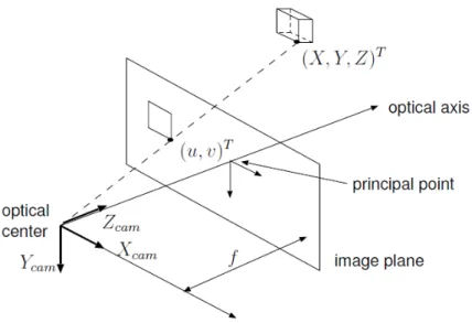
In this thesis we assume that the lens distortion effects of the input images have already been corrected [129], resulting in the standard projective pinhole camera model for projecting 3D points into 2D image space.
Figure 2.4: Pinhole camera model with the projection of a 3D point (X, Y, Z)T
˜ p2D = [K|03]·Tcamworld·p˜3D u v w = fx 0 px 0 0 fy py 0 0 0 1 0 · r11 r12 r13 tx r21 r22 r23 ty r31 r32 r33 tz 0 0 0 1 · X Y Z 1 x y = u w v w with Tcam
world denoting the transformation of the world coordinate origin to the
loca-tion of the camera center andKbeing the intrinsic matrix, containing the calibration parameters from (usually offline) calibration [129],[42]). In case the camera is al-ready placed at the world coordinate origin, the projection of a 3D point into 2D image space reduces to
˜ p2D = [K|03]·p˜cam3D u v w = fx 0 px 0 0 fy py 0 0 0 1 0 · X Y Z 1 x= X·fx Z +px y= Y ·fy Z +py
Push broom camera - RPC model
For an image taken with a push broom camera each image line is taken at a differ-ent instance of time (see Figure 2.5). The exterior oridiffer-entation parameters, i.e. the rotation angles and the position of the perspective center depend on the acquisi-tion time and therefore change from scan line to scan line. The interior orientaacquisi-tion parameters, which comprise the focal length, the principal point location, the lens distortion coefficients, and other parameters directly related to the physical design of the sensor, are in general the same for the entire image. A generic push broom camera model can be expressed by modified collinearity equations in which all ex-terior orientation parameters are defined as a function of time (see e.g. [1], [69], [3], [4]). Nowadays, the RPC model is used for many satellites - only very few have to be modeled by their exact sensor model.
The model for projecting a 3D point j to 2D image space i is given by
xi,j = Pi1(Xj, Yj, Zj) Pi2(Xj, Yj, Zj) , yi,j = Pi3(Xj, Yj, Zj) Pi4(Xj, Yj, Zj) . (2.5)
Figure 2.5: Push broom camera model - image taken from [39]. The 2D image is acquired line-wise.
withxij, yij being the normalized (offset and scaled) image coordinates andXj, Yj, Zj
the corresponding object point coordinates, which refer to normalized latitude, lon-gitude, and altitude. The polynomials are
Pi1(X, Y, Z) =(a1, a2, a3, a4, a5, a6, a7, a8, a9, a10,
a11, a12, a13, a14, a15, a16, a17, a18, a19, a20)·
(1, Y, X, Z, Y X, Y Z, XZ, Y2, X2, Z2, XY Z, Y3, Y X2, Y Z2, Y2X, X3, XZ2, Y2Z, X2Z, Z3)T Pi2(X, Y, Z) =(b1, b2, b3, b4, b5, b6, b7, b8, b9, b10, b11, b12, b13, b14, b15, b16, b17, b18, b19, b20)· (1, Y, X, Z, Y X, Y Z, XZ, Y2, X2, Z2, XY Z, Y3, Y X2, Y Z2, Y2X, X3, XZ2, Y2Z, X2Z, Z3)T Pi3(X, Y, Z) =(c1, c2, c3, c4, c5, c6, c7, c8, c9, c10, c11, c12, c13, c14, c15, c16, c17, c18, c19, c20)· (1, Y, X, Z, Y X, Y Z, XZ, Y2, X2, Z2, XY Z, Y3, Y X2, Y Z2, Y2X, X3, XZ2, Y2Z, X2Z, Z3)T Pi4(X, Y, Z) =(d1, d2, d3, d4, d5, d6, d7, d8, d9, d10, d11, d12, d13, d14, d15, d16, d17, d18, d19, d20)· (1, Y, X, Z, Y X, Y Z, XZ, Y2, X2, Z2, XY Z, Y3, Y X2, Y Z2, Y2X, X3, XZ2, Y2Z, X2Z, Z3)T (2.6)
where Pi1, Pi2, Pi3, Pi4 are cubic functions in object space coordinates, X, Y, Z are
normalized object space coordinates (latitude, longitude, altitude) and xij, yij are
normalized image space coordinates. For a more detailed description of the RPC model, we refer to the work of [39] and [40].
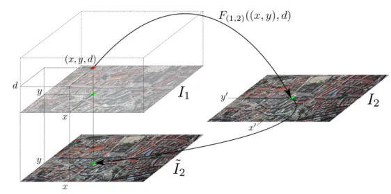
Unified trilinear interpolation model
Since the camera models can differ a lot in their complexity and their projective functions have to be evaluated numerous times, we pursue a different strategy es-pecially for the satellite based RPC model. We establish the epipolar geometry between two images I1 and I2 directly by evaluating the function F(1,2)(x, d), which
projects a pixel x from I1 to I2 using the depth d, for every single pixel of I1 ∈ Ω
and every possible depth d∈D individually.
Especially for push broom images and the RPC camera model, evaluation of
F(1,2)(x, d) for every pixel x and depth hypothesis d is computationally very
ex-pensive and cannot be used in practice. We therefore compute F(1,2)(x, d) only for
a sparse (and uniformly distributed) set of grid points in Ω×Dspace. For all other points we interpolate the projected pixel coordinates by using trilinear interpolation (Figure 2.7). The creation of this lookup-table L is done iteratively starting with a very coarse 10×10×10 grid whose resolution is increased until the reprojection error of the in-between grid points gets smaller than a specified threshold. This allows us to use arbitrary complex camera models while the time for a coordinate transfer (x, d)→F(1,2)(x, d) still is the one needed for a trilinear interpolation using
the lookup table, which can be implemented efficiently.
To furthermore reduce the need for rotational invariant cost functions we apply a plane-sweep approach [23] for computing the image matching cost functions. Given a depthd, we sweep over the reference imageI1, sample imageI2 at the
correspond-ing image position (x0, y0) and copy the obtained color/intensity to an image ˜I2 at
the same position (x, y) as in the reference image. When computing the matching costs of a depth hypotheses d and the whole image I1, we simply evaluate the cost
function at the same position (x, y), using the same local support window in both
I1 and I2. Note that the whole process runs independently for each pixel of I1 and
Figure 2.6: For a coordinate (x, y) in image I1 and the depth d, obtain the
cor-responding coordinate (x0, y0) in image I2 by trilinear interpolation in the sparse lookup tableL, sample the pixel color/intensity and copy it to the warped image ˜I2
at position (x, y). In short notation: ˜I2 =I2(x0, y0) =I2(F(1,2)((x, y), d)).
Figure 2.7: Trilinear interpolation
Image Matching Cost Functions
Many dense stereo reconstruction algorithms exhaustively compute a matching qual-ity for every pixel of a reference image and its possible projections in any other image for every depth hypothesis. Computing such dissimilarity measures of two image positions has the challenging task of fulfilling the two competing requirements of a) being as fast as possible and b) as descriptive / disjunctive as possible. Since we perform an exhaustive search over all depths and each pixel, we have to compute
the full cost volume, which for a standard example of 1024×768 images and 128 depths sums up to slightly more than 100 million dissimilarity computations. At the same time, the dissimilarity measure must be descriptive enough to reduce false matches to a minimum.
Due to the speed requirement, typical dissimilarity measures (also called cost func-tion) in dense stereo are: Absolute Differences (AD), Normalized Cross Correlation (NCC), Birchfield-Tomasi measure [8], Mutual Information [116] and Census trans-form [125]. These are easy to compute, but not very descriptive and therefore prone to false matches.
Of the advanced and more descriptive features (mainly used in image recognition) like SIFT [67], SURF [2], BRIEF [17], BRISK [64] only the DAISY descriptor [114] showed a somewhat acceptable speed for using it in dense stereo reconstruction. Due to some invariance against rotation, scaling and simple radiometric changes, using the DAISY descriptors (or any other of the abovementiond features) yields very good results for wide-baseline stereo, where some simple dissimilarity measures fail because of the large perspective differences. This property makes them good candidates for matching remote sensing stereo images. Unfortunately, as a result of a larger local support window, spatially very closely related pixels have simi-lar (DAISY) descriptors and can’t be distinguished very clearly, which results in a blurry reconstruction of sharp depth discontinuities, occurring for example at the sides of high buildings. For more detailed evaluations of different cost functions, see e.g. the surveys in [99], [112], [48], [49]. Due to the nature of our epipolar geometry model and the plane-sweep approach (Section 2.1.2), it is not necessary for the cost function to be rotational invariant. Also the scale invariance can be neglected for standard dense stereo reconstruction as in our case, where all images of a scene are taken from a similar distance.
(a) I1 with patch (green grid) cen-tered atx1 (red pixel)
(b) I2 with patch centered atx2
Normalized Cross Correlation
The normalized cross correlation is basically the prototype for image matching based on spatial support windowsW (see Figure 2.8) around the pixel positions to compare and is invariant to additive and multiplicative illumination changes.
CN CC(x1,x2) =
P
[i,j]∈W(I1(x1+ [i, j])−µ1(x1)))·(I2(x2+ [i, j])−µ2(x2)))
σ1(x1)·σ2(x2)
CN CC(x, d) = CN CC(x, F(1,2)(x, d)) (2.7)
with µi being the mean intensity of the image patch located at the respective
posi-tions xi and σi the standard deviations accordingly.
Modified Census Transform
The Census transformCT as described in [125] is a non-parametric transform which encodes the local image structure within a small patch around a given pixel. It is defined as an ordered set of comparisons of intensity differences and therefore invariant to monotonic transformations which preserve the local pixel intensity order:
ξ(I(x), I(x0)) = 1 if I(x0)< I(x) 0 otherwise (2.8) CT(I,x) = O [i,j]∈W ξ(I(x), I(x+ [i, j])) , (2.9)
for an ordered set of displacements W ⊂ R2 and the operator N
concatenating the binary values of ξ to a binary string. Image matching is then performed by comparing the resulting binary vectors at different image positions. However, the Census transform strongly depends on the center pixel and a slight variation of its intensity can cause the descriptor to vary significantly. We address this issue by using the following (robustified) modification of the Census transform
M CT(I,x) = O
[i,j]∈W∪[0,0]
ξ( ¯I(x), I(x+ [i, j])) , (2.10)
where we replaced the intensity of the center pixel by a weighted average of the intensities in its direct 4-neighborhood (see Figure 2.9). A similar modification is used by [32] for face detection.
The matching cost of different Census vectors s1, s2 is then computed as their
Hamming distance dH(s1, s2) – number of differing bits – where highest matching
quality is achieved for minimal Hamming distance. To simplify further usage of the matching costs, we scale them to the real-valued interval [0,1] by dividing through
Figure 2.9: Left: The displacement field D used for computing a 61-Bit census transform of the black center pixel. The size of D was chosen deliberately, as to fit in a 64-Bit variable. Right: The weights for computing the center pixel intensity
¯
I(x).
the maximal cost maxi,j{dH(si, sj)}, which equals the number of pixels in the
dis-placement field D. CM CT(x, d) = dH M CT(I1,x), M CT(I2, F(1,2)(x, d)) maxi,j{dH(si, sj)} (2.11)
Having a large support window for the Census transform, as shown in Figure 2.9, increases the robustness of the matching function against mismatches, espe-cially when searching through a large range of depths. The support window size of the Census transform is typically 5×5, 7×7, 7×9, or circular spatial structure like Figure 2.9, because due to efficient implementation issues, the resulting binary vectors then fits into 32 or 64 bit variables.
On the other hand, this window-based matching faces several drawbacks: The depth within the window is assumed to be constant and the results therefore are biased towards fronto-parallel surfaces. For the same reason, the resulting depth map gets blurry along discontinuities.
To limit the influence of these drawbacks, the window-based cost function of Equa-tion 2.11 can be combined (weighted sum) with a pixel-wise second cost funcEqua-tion using e.g., absolute difference of the intensity values or mutual information.
Mutual Information
Mutual Information [116] has already proven to be a good choice as pixel-wise match-ing cost function ([51], [44]) and is based on the joint entropy of the involved images. For combination with other cost functions, we normalize the MI cost function to [0,1]
CM I(x, d) = 1−
˜
CM I(x, d)−minx,d{C˜M I(x, d)}
maxx,d{C˜M I(x, d)} −minx,d{C˜M I(x, d)}
with
˜
CM I(x, d) =miI1,I2(I1(x), I2(F(1,2)(x, d)) ) (2.13)
and miI1,I2 being the mutual information according to [116]. As Equation 2.13
requires knowledge of the depthd a priori, a hierarchical approach is used to get a good estimate for ˜CM I (see [44]).
Adaptive Support Weights
Window-based image matching suffers from the ”foreground fattening” phenomenon when support windows are located on depth discontinuities, such as partially cov-ering a roof top and the adjacent street. To limit this effect, we locally aggregate the raw image matching cost(x1,x2) of two pixel locations x1 and x2 – e.g., from
Equation 2.7, 2.11, 2.12 – using adaptive support-weights [124] for corresponding pixelsp in I1 and q inI2: C(p,q) = P ˜ p∈Np,q˜∈Nq[w(p,p˜)·w(q,q˜)·cost(˜p,q˜)] P ˜ p∈Np,q˜∈Nq[w(p,p˜)·w(q,q˜)] (2.14)
The weights w(p,q) are based on color differences ∆col(p,q) and spatial distances
∆dist(p,q), w(p,q) = exp −∆col(p,q) γcol −∆dist(p,q) γdist , (2.15)
which are open for tuning but usually reside in the range of γdist = 4 (= radius of
the support window) and γcol = 5.0 for 8-bit images (γcol = 20.0 for 11-bit images
respectively). As this local aggregation favors fronto-parallel surfaces, we keep this radius relatively small (4 pixel), to keep a balance between increased accuracy along discontinuities and not ”over-favoring” fronto-parallel surfaces.
Figure 2.10: Basic scheme for the adaptive support-weights as described in Equation 2.14. In a local neighborhood around the considered matching pixel positionspand
q, the matching cost of all possible matching coordinates are weighted and summed up, according to the scheme described in this Section 2.2.4.
(a) (b)
Figure 2.11: (a) Input image with center pixel marked by rectangle. (b) Corre-sponding support-weights incorporating both color and spatial distance (brighter pixel corresponding to larger support-weights). Image taken from [124].
Shortcomings
As much effort as one might put into image matching cost functions, there are many cases where image matching is basically not possible - see Figure 2.12 for some examples. The so-called data term is too weak, misleading or ambiguous for reliable estimation of the true optimal solution using image matching alone (see Figure 2.13). Two overcome this problem an additional regularization term is used for reconstruction of piecewise smooth solutions - which will be described in the following section.
(a) Repetitive texture along the shingles of the roofs
(b) Textureless regions along the flat roof
(c) Sensor oversaturation and specular reflections
(a) Reference image with selected points: unique (U), homogeneous (H), occluded (O).
(b) Second matching image with search space along epipolar lines.
(c) Image matching cost functions for each of the three considered points (U,H,O): pixelwise absolute difference (AD0), Census 5×5 (CEN), and weighted mean of both (ADC).
Figure 2.13: Image matching cost functions for selected points and their 3D search space along the corresponding epipolar lines. For details on improving the quality of the data term via multiple measurements see Chapter 4.
Total Variation Regularization
Since the raw image matching costs are still prone to mismatches and noise, it is a bad choice to solve for the depth map pixel-wise by choosing the depth with minimum matching cost (compare Figure 2.3(a)). Adding additional smoothness priors is a well established technique to mitigate the effect of erroneous data terms, forcing the depth map to be locally smooth.
u∗ = arg min u Z Ω Edata(u(x)) +Esmooth(u(x)) dx (2.16) = arg min u Z Ω C(u(x)) +λ·h(u(x)) dx
The data term C still measures the quality of the matching image patches and is now balanced against a smoothing functionalh with a controllable scalar weighting factor λ. Compared to the pixelwise solution of Equation 2.4, this energy is non-trivial to solve, since the smoothness constraints (implied by the smoothing function
h) are typically based on first- or second-order derivatives of the depth map and therefore cannot be optimized pixelwise anymore. The choice of the data term and smoothness energy functional are the most important issues, since they both affect the property of preserving the original signal as well as being able to solve the resulting optimization problem accurately and efficiently. Typically, the data term is not convex in the variable u to solve for, while the regularization term implies difficulties for an efficient optimization scheme.
Total Variation
We first give a formal definition of the total variation and its higher order counter-part the total generalized variation and afterwards illustrate their properties in an example of denoising 2D data.
Definition 1 Ck functions
Let k be a non-negative integer. The function f is said to be of class Ck if the
derivatives f0, f00, ..., f(k) exist and are continuous. The function f is said to be of class C∞, or smooth, if it has derivatives of all orders.
Definition 2 Lp space
The space of p-integrable functions is defined as
Lp(Ω) := ( f : Ω→R| Z Ω |f|p dx 1/p <∞ ) (2.17)
Definition 3 Sobolev space Wk,p
The Sobolev space Wk,p(Ω) is defined to be the set of all functions u∈Lp(Ω) such that for every n-tuple α with |α| ≤ k, the weak partial derivative Dαu belongs to
Lp(Ω)
Wk,p(Ω) ={u∈Lp(Ω) :Dαu∈Lp(Ω) ∀|α| ≤k}. (2.18) Intuitively, a Sobolev space is a space of functions with sufficiently many derivatives for e.g., partial differential equations and is equipped with a norm that measures both the size and regularity of a function.
Definition 4 Weak partial derivative
Given an open set Ω ⊂Rn, a function f ∈ L1 is weakly differentiable with respect
to xi if there exists a function gi ∈L1 such that Z Ω f ∂iφ dx=− Z Ω giφ dx, (2.19)
for all functions φ being infinitely differentiable and with compact support in Ω, i.e. φ ∈Cc∞(Ω). The functiongi is called the weak ith partial derivative of f, and
is denoted by ∂if.
Weak derivatives generalize the concept of the (strong) derivative of a function for functions which are not differentiable, but only integrable. The main idea behind the weak derivative is that Equation 2.19 allows to shift the differential operator from one variable to another one which is defined to be always differentiable.
Definition 5 Total Variation
Given a function u ∈ L1(Ω) on a bounded domain Ω ⊂ Rn with n ≥ 2, the total
variation of u is defined as TV(u) := sup Z Ω u(x)·div(φ(x)) dx : φ ∈Cc1(Ω,Rn), ||φ||∞ ≤1 (2.20) with div(φ(x)) = n X i=1 ∂φi ∂xi (x) (2.21)
and if u∈W1,1(Ω), see e.g. [21], the total variation ofu can be written as
TV(u) =
Z
Ω
Definition 6 Total Generalized Variation
The total generalized variation of order k with weightsα is defined as
TGVkα(u) := sup Z Ω u·divkφdx :φ∈Cck(Ω,Symk(Rn)), (2.23) ||divlφ||∞≤αl, l = 0, ..., k−1
with k ≥1 and α0, ..., αk−1 ≥0. Symk(Rn) denotes the space of symmetric tensors
of order k with arguments in Rn. Note that for k = 1 and α >0 it holds that
TGV1α(u) = sup Z Ω u·divφdx : φ∈C1(Ω,Sym1(Rn)),||φ||∞≤α =α·TV(u) (2.24)
implying that TGV is indeed a generalization of TV.
Depth map denoising example
Due to its simplicity we use the application of depth map denoising to illustrate the effects of total variation regularization as well as different norms for the data term. Given a corrupted 2D depth map f, we want to obtain denoised 2D data u.
Tikhonov model
The quadratic model (or Tikhonov model [113]) is one of the earliest and simplest regularization methods used for ill-posed problems. It is defined as the quadratic variational problem min u Z Ω (u−f)2 dx + λ Z Ω |∇u|2 2 dx , (2.25)
The quadratic model tries to find a smooth solutionuwhich minimizes the squared distance to the observations f. Being quadratic in u, the Tikhonov model poses a simple optimization problem, but it leads to an oversmoothing of edges and the quadratic data term is not robust against strong outliers in the observed data. For this reason, we do not consider this model at all and only mention it here for sake of completeness.
ROF model
The seminal paper of [96] introduced the Rudin-Osher-Fatemi model (ROF-model) as an edge preserving 2D image restoration model by applying total variation as
regularization term min u Z Ω (u−f)2 dx + λ Z Ω |∇u|2 dx . (2.26)
Note that the ROF model is convex and has a unique global minimizer.
TV-L1 model
By substituting the quadratic data term in the ROF model with it’s L1 pendant we
arrive at the TV-L1 model
min u Z Ω |u−f|dx + λ Z Ω |∇u|2 dx . (2.27)
The difference to the ROF model is that discontinuities in the data are well pre-served, since deviations in the data term are not penalized quadratically anymore, but only linearly. This makes the TV-L1 model much more robust to outliers in the
data term. One can say that the ROF model is a good choice if the assumed noise is of Gaussian nature and the TV-L1 model should be used if white noise (outliers) are present in the data. The TV-L1 model unfortunately is not strictly convex anymore
and does not have a unique global minimizer.
TV-Huber model
The advantage of choosing the L1 norm for Esmooth = |∇u|1 however does not
come without cost. As shown in Figure 2.14, minimizing the Total Variation leads to staircasing effects on otherwise smooth data in the resulting reconstruction. To overcome this issue a slight modification of the regularization functional by replacing the L1 norm with the Huber loss (see Figure 2.15 and Equation 2.29 below) was
used by [120] to regularize optical flow estimation.
min u Z Ω |u−f| dx + λ Z Ω |∇u|h dx (2.28)
The Huber loss still preserves the main advantage of theL1 norm for penalizing
deviations in the first order derivative only linearly, however small deviations are now penalized quadratically (see Equation 2.29) leading to smooth surfaces and mitigating the stair casing effect.
Definition 7 Huber loss
Figure 2.14: Staircasing effect of Total Variation. Without any additional data
u between the positions x1 and x2, regularization via minimization Total Variation
does not have a unique solution as every dashed line has the same amount of total variation in u. The gray line corresponds to a smooth regularization between the data points.
(quadratic penalties as in L2-norm in a local environment and linear penalties L 1
for outliers). It is defined as
|x|h = |x|2 2h if |x| ≤h |x| − h 2 if |x|> h (2.29)
Furthermore, the Huber loss is fully differentiable with
Figure 2.15: Huber loss |x|h with h = 1.0
∂|x|h ∂x = ( 2|x|x |x| 1 2h if |x|< h x |x| else = x h if |x|< h sgn(x) else (2.30)
![Figure 1.6: Exemplary data from the Middlebury dataset [98]](https://thumb-us.123doks.com/thumbv2/123dok_us/1287386.2672759/24.892.141.761.181.647/figure-exemplary-data-middlebury-dataset.webp)
![Figure 2.5: Push broom camera model - image taken from [39]. The 2D image is acquired line-wise.](https://thumb-us.123doks.com/thumbv2/123dok_us/1287386.2672759/36.892.258.642.179.436/figure-push-broom-camera-model-image-taken-acquired.webp)