Ultrasound Elastography: Time Delay Estimation
Hoda Sadat Hashemi
A Thesis in
The Department of
Electrical and Computer Engineering
Presented in Partial Fulfillment of the Requirements for the Degree of
Master of Applied Science (Electrical Engineering) at Concordia University
Montr´eal, Qu´ebec, Canada
July 2017
c
C
ONCORDIAU
NIVERSITY School of Graduate StudiesThis is to certify that the thesis prepared
By: Hoda Sadat Hashemi
Entitled: Ultrasound Elastography: Time Delay Estimation
and submitted in partial fulfillment of the requirements for the degree of
Master of Applied Science (Electrical Engineering)
complies with the regulations of this University and meets the accepted standards with respect to originality and quality.
Signed by the Final Examining Committee:
Chair Dr. R. Raut External Examiner Dr. N. Bouguila Examiner Dr. M. O. Ahmad Supervisor Dr. H. Rivaz Approved by Dr. W. E. Lynch, Chair
Department of Electrical and Computer Engineering
2017
Dr. A. Asif, Dean
Abstract
Ultrasound Elastography: Time Delay Estimation Hoda Sadat Hashemi
A critical step in quasi-static ultrasound elastography is estimation of time-delay between two frames of Radio-Frequency (RF) data that are obtained while tissue is undergoing deforma-tion. This thesis presents a novel technique for Time-Delay Estimation (TDE) ofall samples of RF data simultaneously. A nonlinear cost function that incorporates similarity of RF data intensity and prior information of displacement continuity is formulated. Optimization of this nonlinear func-tion involves searching for TDE of all samples of RF data, rendering the optimizafunc-tion intractable with conventional techniques given that the number of variables can be approximately one mil-lion. Therefore, the optimization problem is converted to a sparse linear system of equations, and is solved in real-time using a computationally efficient optimization technique. We call our method GLUE (GLobal Ultrasound Elastography), and compare it to Dynamic Programming Analytic Min-imization (DPAM) (Rivaz, Boctor, Choti, & Hager, 2011) and Normalized Cross Correlation (NCC) techniques. We test our method on simulation, phantom, andin-vivodata. The results show that the proposed method outperforms both DPAM and NCC techniques. In another proposed method, we assume tissue deformation can be efficiently approximated by an affine transformation, and hence call our method ATME (Affine Transformation Model Elastography). The affine transformation model is utilized to obtain initial estimates of axial and lateral displacement fields. The nonlin-ear cost function of GLUE method is used to fine-tune the initial affine deformation field. Results on simulation and RF data we collect fromin-vivopatellar tendon and medial collateral ligament (MCL), show that ATME can be used to accurately track tissue displacement.
Acknowledgments
My appreciation, first goes to my knowledgeable, innovative and genius supervisor, Prof. Has-san Rivaz, for his awesome supervision which brought me a wonderful academic life at Concordia University. His dedication and full support above all his awesome guidance and novel ideas have helped me to accomplish this work. His energetic personality consistently motivated me to push forward my research. I would never forget his affection and warmth throughout my research period, and I am deeply grateful for them.
I would like to thank my colleagues and friends in the research group of my professor, IM-PACT group, for their great discussions. Also, I do appreciate Dr. Mathieu Boily and Dr. Paul A. Martineau from McGill University, and also Dr. Robert Kilgour from Concordia exercise science department for their invaluable discussions and collaborations in my work.
I would like to acknowledge the financial support from the Richard and Edith Strauss Canada Foundation throughout my graduate work at Concordia University.
Finally, I would like to express my gratitude to my parents and sisters for their love and lasting supports. I would like to thank my grandmother for her continuous encouragements and fervent hope.
Contents
List of Figures vii
List of Tables x
1 Introduction 1
1.1 Ultrasound Imaging . . . 1
1.2 Ultrasound Elastography . . . 4
2 Global Time-Delay Estimation in Ultrasound Elastography 7 2.1 Introduction . . . 7
2.2 Methods . . . 11
2.2.1 Dynamic Programming Analytic Minimization (DPAM) . . . 11
2.2.2 Global Time-Delay Estimation (GLUE) . . . 13
2.3 Experiments and Results . . . 17
2.3.1 Simulation Results . . . 18
2.3.2 Phantom Results . . . 20
2.3.3 In-vivo Results . . . 20
2.4 Discussion . . . 27
2.5 Conclusion . . . 28
3 Efficient Estimation of Tissue Displacement Using an Affine Transformation Model 29 3.1 Introduction . . . 29
3.3 Experiments and Results . . . 33
3.3.1 Simulation Experiments . . . 33
3.3.2 in-vivoExperiments . . . 33
3.4 Conclusion . . . 38
4 Conclusion and Future Work 39 4.1 Conclusion . . . 39
4.2 Future Work . . . 40
List of Figures
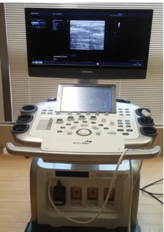
Figure 1.1 An Alpinion E-CUBE 12R ultrasound system. . . 2 Figure 1.2 Ultrasound images. . . 2 Figure 1.3 Ultrasound Transducers. (a), Image courtesy of: (Abu-Zidan, Hefny, Corr,
et al., 2011), (b), Image courtesy of: https://pics-about-space.com/ . . . 3 Figure 1.4 Ultrasound doppler image of the blood flow. Image courtesy of: (Sato et al.,
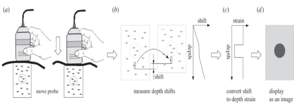
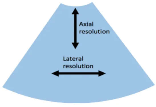
2015) . . . 4 Figure 1.5 Quasi-static procedure. Image courtesy of (G. Treece et al., 2011) . . . 4 Figure 1.6 Axial and lateral resolution on the image produced by a sector scanner. . . . 5 Figure 2.1 Comparison of NCC, DPAM and GLUE algorithms, with the corresponding
strain images in the second row. In (a) to (c), each circle shows an RF sample that is utilized in TDE. Each grid point corresponds to a sample in RF data. Few samples are shown here to ease visualization; real RF data contains significantly more samples. In (a), few samples are grouped together to form a window, which is used to calculate NCC. The displacement of all samples in an entire RF-line in DPAM (b) or the entire image in GLUE (c) are estimated together. (d) to (f) show strain images of a homogeneous phantom. Note that the average strain is8%. GLUE substantially outperforms both NCC and DPAM by utilizing all data in the RF-frame. 10
Figure 2.2 Field II and FEM simulation results. (a) is the axial ground truth strain. (b) to (d) show the axial strain images of the first simulation. (e) is the lateral ground truth strain. (f) to (h) show the lateral strain images of the first simulation. GLUE substantially outperforms NCC and DPAM in all results. Target and background windows used for CNR calculation are shown in red. The SNR is calculated for the background window. . . 18 Figure 2.3 Field II and FEM simulation results. A vertical slippage exists in the motion
field at the middle of the image. (a) is the first ultrasound image. (b) to (d) are the axial strain images. (e) is the second ultrasound image. (f) to (h) are the lateral strain images. Target and background windows used for CNR calculation of the GLUE results are shown in red. The SNR is calculated for the background window. 19 Figure 2.4 Results of the phantom experiment. Axial and lateral strain images as well
as the target and background windows (in red) for calculation of SNR and CNR are shown (see Table 2.3 for results). The hard lesion is spherical and has a diameter of 1 cm. The axial and lateral strain scales are identical for NCC, DPAM and GLUE to ease comparison, and are shown in the right column. . . 21 Figure 2.5 In-vivo images of the ablation lesion acquired after ablation of liver
tu-mours. Each row corresponds to one patient. The first column shows ultrasound images, and the second and third columns respectively show the results of DPAM and GLUE. The ablation lesion is marked with red arrows, and is clearly visible in strain images. CT images with the delineated ablation lesions are shown in the right column. . . 23 Figure 2.6 B-mode and strain images of the patient data before ablation. First and
sec-ond rows respectively correspsec-ond to patients 2 and 3. The red arrows point to the tumours. The strain images provide a substantially improved visualization of the tumours compared to the B-mode ultrasound images. . . 25
Figure 2.7 B-mode and strain images of patient 4 before ablation. (a) shows B-mode image, and (b) and (c) show the strain images from the DPAM method using US 1 and 2 frames (for b) and US 3 and 4 frames (for c). (d) shows the motion of the probe and the variation in the diameter of the arteries due to the heart beat. (e) and (f) show results of the GLUE method. (g) is the arterial phase and (h) is the venous phase contrast CT images. The tumor is marked with red arrows in (b), (c), (e), and (f). . . 26 Figure 3.1 Displacement field between a pair of ultrasound images in a uniform tissue. 30 Figure 3.2 Field II and finite element simulation results. (a) and (b) show the axial and
lateral ground truth displacement images of the simulation experiment. (c) and (d) are the corresponding axial and lateral displacement fields obtained from ATME. . 32 Figure 3.3 Distal tendon motion during force flexion experiment. (a) and (b) show axial
and lateral displacements. (c) is the B-mode image and red arrows represent the strain directions in the tendon. (d) and (e) depict the axial strain and magnified strain directions respectively. . . 34 Figure 3.4 MCL during pure valgus stress experiment. (a) and (b) show axial and lateral
displacements. (c) is the B-mode image and red arrows represent the strain direc-tions in the MCL. (d) and (e) depict the axial strain and magnified strain direcdirec-tions respectively. . . 36 Figure 3.5 title of the figure . . . 37
List of Tables
Table 2.1 The SNR and CNR values of the simulation experiment. Target windows (5mm X 5mm) and background windows (3mm X 3mm) used for CNR calcula-tion are shown in Figure 2.2. The SNR is calculated in the background window. Maximum values are in bold font. . . 20 Table 2.2 The SNR and CNR values of the simulation experiment. Target windows
(5mm X 5mm) and background windows (3mm X 3mm) used for CNR calculation are shown in Figure 2.3. The SNR is calculated in the background window. . . 20 Table 2.3 The SNR and CNR of the strain images of the experimental phantom. Target
and background windows used for CNR calculation are shown in Figure 2.4. The SNR is calculated for the background window. Maximum values are in bold font. . 22 Table 2.4 The SNR and CNR values of the strain images of the in-vivo data in
Fig-ure 2.5. The SNR is calculated for the background window of size 6 mm×6 mm. Maximum values are in bold font. . . 22 Table 2.5 The SNR and CNR of the strain images of thein-vivodata in Figures 2.6 and
2.7. The CNR calculated for the target and background window each of size 6mm
×6mm. The SNR is calculated for the background window. Maximum values are in bold font. . . 24 Table 3.1 The SNR and CNR of the strain images of Fig. 3.5. Maximum values are in
Chapter 1
Introduction
This chapter provides a brief summary on some ultrasound imaging principles. We then focus on ultrasound elastography which is the main concentration of this thesis.
1.1
Ultrasound Imaging
Medical imaging has brought great advances in disease diagnostic and treatment during recent decades. Ultrasound is sound waves which have higher frequencies than the range of human hearing (20 Hz-20kHz). It has meanwhile emerged as an attractive medical imaging approach due to its numerous advantages. Anatomy, tissue characterization, and dynamic movement of organs can be investigated using ultrasound. Furthermore, it is safe, easy to use, portable and cost efficient.
In Figure 1.1, an Alpinion E-CUBE 12R ultrasound system is shown. One of the important parts of the ultrasound imaging system is the transducer probe which consists of piezoelectric material or crystals. Applying electrical voltage to these crystals produces acoustic signals that travel outward. The waves propagate into the body and hit the boundary between different tissues. Some reflections of acoustic waves back scatter to the probe, whereas, the rest penetrate deeper into the tissue and reflect after hitting another boundary. The transducer receives the reflected waves and sends them back to the machine as the electrical currents. By using the speed of sound and arrival time of each reflection to the probe, the distance between the probe and tissue is calculated. The intensities and distances of the echoes are shown on the screen as an ultrasound image as illustrated in Figure
Figure 1.1: An Alpinion E-CUBE 12R ultrasound system.
(a) Patellar tendon (b) Rotator cuff
Figure 1.2: Ultrasound images.
1.2. (a) is an ultrasound image of patellar tendon of the knee and (b) shows a rotator cuff tendon ultrasound image.
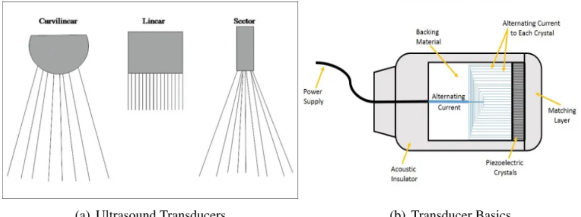
(a) Ultrasound Transducers (b) Transducer Basics
Figure 1.3: Ultrasound Transducers.
(a), Image courtesy of: (Abu-Zidan et al., 2011), (b), Image courtesy of: https://pics-about-space.com/
frequency of the probe specify the transducer performance. The resolution of the image and wave penetration depth are dependent to the frequency of the produced acoustic wave. On the other hand, the probe field of view is connected to its shape. The most utilizable probes are linear, curvilinear, and phased array (sector) probes (Figure 1.3, (a)). A linear probe works with high frequency waves, and consequently provides high resolution images of structures near the body surface. The generated ultrasound images on the screen are generally in rectangular shape (Figure 1.2, (a)). The usage of this probe is in superficial imaging such as: vascular system, skin and soft tissue, musculoskeletal structures, testicular assessment, interstitial fluid diagnosis, ocular ultrasound, breast and thyroid imaging. Curvilinear probe employs lower frequency letting the sound penetrate deeper. It produces pie shaped images, and also has wide field of view due to its curved shape which is ideal for intra-abdominal imaging and organ diagnosis. Phased array probe generates slice of pie shaped images (Figure 1.4). It has small footprint and a wide field of view at the deep parts using low frequency. These features make it compatible for imaging the cardiac structures in the chest through a small acoustic window between the ribs, transesophageal applications, and brain diagnosis.
Emission of ultrasound waves from the probe can be either interrupted or continuous. Inter-rupted emission results in the brightness mode (B-mode) images (Figure 1.2). In B-mode ultra-sound, a 2D image is produced on the screen while the transducer simultaneously scans a plane
Figure 1.4: Ultrasound doppler image of the blood flow. Image courtesy of: (Sato et al., 2015)
Figure 1.5: Quasi-static procedure. Image courtesy of (G. Treece et al., 2011)
through the body. However, continuous emission generates Doppler mode that is ideal for mesur-ment of blood velocity utilizing the Doppler effect as shown in Figure 1.4.
1.2
Ultrasound Elastography
Elastography performs tissue characterization and measurement of the elastic properties of the tissue. In fact, mechanical stress caused by a probe (external) or ultrasonic radiation force (internal) is applied to the tissue. Local tissue deformation is calculated which provides the information about mechanical properties of the tissue. So, it can recognize healthy from unhealthy tissue through
Figure 1.6: Axial and lateral resolution on the image produced by a sector scanner.
stiffness measurements. The most noted ultrasound elastography techniques are: Quasi-static Elas-tography, Shear Wave Elasticity Imaging (SWEI), Supersonic Shear Imaging (SSI), Acoustic Radi-ation Force Impulse imaging (ARFI), and Transient Elastography (Bamber et al., 2013; Gennisson, Deffieux, Fink, & Tanter, 2013; Tanter & Fink, 2014). In this thesis, we focus on quasi-static elas-tography or stain imaging. In Figure 1.5, an approximately static force is applied on the tissue by the probe moving continuously with low velocity. Before and after compression images are compared using a tracking method. The shifts between the locations of the samples in pre- and post-compression images are calculated and stored as the displacement map. Consider the overall change in axial length of tissue asdz. Thus, the post compression time is 2dzc . Local axial strain can be calculated as:Sn= tn+12dz−tn
c
wheretnis the time shift for segment or time windown. Similarly, the 2D strain can be calculated for the lateral direction. Axial and lateral ultrasound image resolu-tion are different. Thus, the axial strain holds better quality than the lateral one. For axial direcresolu-tion, the resolution is defined as the shortest distance of two distinguishable structures lying in the beam axis that depends mainly on sampling frequency. However, the lateral resolution determined by the beam width and refers to shortest distance of two distinguishable structures which are perpendicular to the beam axis (Figure 1.6).
The general objective of this thesis is to estimate the displacement field between two ultra-sound frames through minimizing a regularized cost function. The cost function incorporates both similarity of RF data intensity and displacement continuity. The regularization coefficients are the elastography parameters which can be tuned in the presettings of the ultrasound machine based
on the application. For every organ, these parameters can be determined by visually inspecting the displacement map. The higher or lower regularization weights are employed to improve noisy displacement map or oversmoothed one, respectively. Finally, we are able to calculate the displace-ment field between two ultrasound images and subsequently find the corresponding strain images revealing mechanical properties of the tissue. The obtained strain images can be used to uncover the invisible tumors and lesions in the initial B-mode images. Furthermore, the strain field is repre-sented by arrows using magnitude and direction of the strain for every point in the image. It clarifies how the tissue actually stretches and in what areas there are more tension as we expect in reality. The method is tested on liver, patellar tendon and Medial Collateral Ligament (MCL) data.
This thesis is organized as follows. In Chapter 2, we will propose a novel technique called GLUE: GLobal Ultrasound Elastography (Hashemi & Rivaz, 2017). We show that GLUE outper-forms state of the art ultrasound elastography methods using simulation, phantom and in-vivo ex-periments. In Chapter 3, we propose an efficient method to find an approximate displacement map between ultrasound images. We refer to this technique as ATME: Affine Transformation Model Elastography (Hashemi, Boily, Martineau, & Rivaz, 2017). We show that ATME efficiently esti-mates an approximate displacement field using phantom andin-vivoexperiments. We conclude this thesis in Chapter 4 with a summary and avenues for future work.
Chapter 2
Global Time-Delay Estimation in
Ultrasound Elastography
2.1
Introduction
As briefly mentioned in the introduction chapter, ultrasound elastography reveals viscoelastic properties of tissue, which are often correlated with pathology, and is therefore of significant clin-ical importance. Elastography has evolved into several different techniques, but it can broadly be grouped into dynamic and quasi-static elastography (Gennisson et al., 2013; Hall et al., 2011; Ophir et al., 1999; Parker, Doyley, & Rubens, 2012; Tang, Cloutier, Szeverenyi, & Sirlin, 2015; G. Treece et al., 2011). Dynamic elastography techniques include shear wave imaging (Bercoff, Tanter, & Fink, 2004) and acoustic radiation force imaging (Nightingale, Soo, Nightingale, & Trahey, 2002), which generate deformation in the tissue using ultrasound and provide quantitative mechanical prop-erties of tissue. This work focuses on quasi-static elastography, and more particularly on free-hand palpation elastography, wherein tissue deformation is slow and is generated by slowly palpating the tissue with the hand-held ultrasound probe.
Free-hand elastography and shear wave elastography each has its own strengths. Free-hand strain imaging does not provide quantitative elasticity measures, unless it is combined with an in-verse problem approach (Babaniyi, Oberai, & Barbone, 2017; M. Doyley, 2012; Goksel, Eskandari, & Salcudean, 2013; Hoerig, Ghaboussi, Fatemi, & Insana, 2016; Mousavi, Sadeghi-Naini, Czarnota,
& Samani, 2014) that solves for tissue elasticity, whereas shear-wave elastography techniques pro-vide quantitative values of tissue elasticity or shear moduli (Catheline, Wu, & Fink, 1999; Song et al., 2012; Tanter et al., 2008). An advantage of freehand strain imaging emanates from the larger displacement fields compared to that of shear-wave elastography, which can lead to less noise in the estimated displacement field. Although elastography techniques vary significantly in the way they generate tissue deformation and in the biomechanical property they investigate, they all require estimation of tissue displacement, commonly referred to as Time-Delay Estimation (TDE) using ultrasound radio-frequency (RF) signal. TDE is challenging and an active field of research due to various sources of noise and signal decorrelation. In this thesis, we focus on TDE in freehand palpation elastography (M. M. Doyley, Bamber, Fuechsel, & Bush, 2001; Hall, Zhu, & Spalding, 2003; Hiltawsky et al., 2001; Lindop, Treece, Gee, & Prager, 2006; Ophir, Cespedes, Ponnekanti, Yazdi, & Li, 1991; Yamakawa et al., 2003). This approach is attractive as it works with traditional ultrasound machines and does not require any additional hardware.
Window-based techniques calculate TDE for small windows (segments) of the RF data, and can be categorized into amplitude- and phased-based. Amplitude-based methods maximize cross correlation or normalized cross correlation (NCC) (Lopata et al., 2009; Nahiyan & Hasan, 2015; Pan et al., 2015; Zahiri & Salcudean, 2006), whereas phase-based methods find the zero-crossing of the phase of the cross correlation (Ara et al., 2013; X. Chen, Zohdy, Emelianov, & O’Donnell, 2004; Lindop, Treece, Gee, & Prager, 2008; O’Donnell, Skovoroda, Shapo, & Emelianov, 1994; Pesavento, Perrey, Krueger, & Ermert, 1999; Yuan & Pedersen, 2015). Window-based displace-ment estimation techniques can also be categorized by the dimensionality of the search range: 1D methods only search in axial directions (Bilgen & Insana, 1996; Dickinson & Hill, 1982; Ophir et al., 1991), and 2D techniques perform a search in both axial and lateral directions (Ebbini, 2006; Friemel, Bohs, & Trahey, 1995; Konofagou & Ophir, 1998; G. M. Treece, Lindop, Gee, & Prager, 2008). Since the underlying displacement field is usually 3D, 2D displacement estima-tion techniques generally outperform their 1D counterparts. The importance of 2D displacement estimation is twofold: it provides more accurate estimates of axial strain (Jiang & Hall, 2015), and it can be used for reconstruction of tissue elastic properties (Babaniyi et al., 2017; M. Doyley, 2012; Goksel et al., 2013; Hoerig et al., 2016; Mousavi et al., 2014). One of the disadvantages of
window-based methods is their sensitivity to signal decorrelation, which can be caused by small out-of-plane motion of the probe or large deformations. Larger windows, approximately of the size 10 ultrasound wavelengths or larger (H. Chen, Shi, & Varghese, 2007; Grondin, Wan, Gambhir, Garan, & Konofagou, 2015), provide more information and hence reduce the estimation variance, but they result in significant signal decorrelation and also decrease the spatial resolution. Reme-dies for these problems have been proposed such as warping the data (Alam & Ophir, 1997; Alam, Ophir, & Konofagou, 1998; Chaturvedi, Insana, & Hall, 1998), which are generally computationally expensive.
An attractive alternative approach to correlation-based methods is minimization of a regularized cost function (Brusseau, Kybic, D´eprez, & Basset, 2008; Hall et al., 2011; Kuzmin, Zakrzewski, Anthony, & Lempitsky, 2015; Maurice & Bertrand, 1999; Pellot-Barakat, Frouin, Insana, & Her-ment, 2004; Rivaz et al., 2008). These methods exploit the prior information that tissue deformation is smooth, and therefore are robust to signal decorrelation. A disadvantage of these methods is their computational complexity, and as such, they are not readily suitable for real-time implemen-tation. Our group proposed a real-time technique for estimating fine subpixel tissue displacement maps using Dynamic Programming and Analytic Minimization (DPAM) of a regularized cost func-tion (Rivaz et al., 2011; Rivaz, Boctor, Choti, & Hager, 2014), whereby displacements of all the samples in an RF-line are estimated simultaneously. This simultaneous estimation results in both more robust and accurate displacement estimates compared to NCC-based methods that only utilize data within a window. In (Rivaz et al., 2011), the subpixel displacement of a seed-line is calcu-lated first, and is used as an initial estimate for neighboring RF-lines. This algorithm, however, has three drawbacks. First, the simultaneous estimation is limited to individual RF-lines, thereby only utilizing a small fraction of the information available from the entire image. Second, displacement estimates are discontinuous between adjacent RF-lines, creating artifacts in the form of vertical streaks in the strain image. And third, displacement estimation in each line depends on the initial estimate, i.e. the displacement of the previous RF-line. Hence, if there is large decorrelation or noise in an RF-line that results in failure of its displacement estimation, the erroneous displacement propagates to the consequent RF-lines. We present herein a novel method for estimating accurate 2D displacement maps wherein the displacement of the entire image is estimated simultaneously.
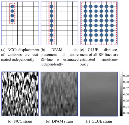
(a) NCC: displacement of windows are esti-mated independently (b) DPAM: dis-placement of entire RF-line is estimated independently (c) GLUE: displace-ment of all RF-lines are estimated simultane-ously
(d) NCC strain (e) DPAM strain (f) GLUE strain
Figure 2.1: Comparison of NCC, DPAM and GLUE algorithms, with the corresponding strain im-ages in the second row. In (a) to (c), each circle shows an RF sample that is utilized in TDE. Each grid point corresponds to a sample in RF data. Few samples are shown here to ease visualization; real RF data contains significantly more samples. In (a), few samples are grouped together to form a window, which is used to calculate NCC. The displacement of all samples in an entire RF-line in DPAM (b) or the entire image in GLUE (c) are estimated together. (d) to (f) show strain images of a homogeneous phantom. Note that the average strain is8%. GLUE substantially outperforms both NCC and DPAM by utilizing all data in the RF-frame.
We call the new method GLobal Ultrasound Elastography (GLUE). Figure 2.1 provides a schematic comparison of three different methods:
(a) Window-based methods, which calculate the displacements of each correlation window inde-pendently typically of the size about 50 samples.
(b) DPAM, which uses the information of an RF-line typically of the size about 1000 samples, to acquire the displacements of all samples of the RF data.
(c) GLUE, which utilizes the information of all image samples typically of the size1000×100 = 105, and calculates TDE of all the samples of the RF frame simultaneously.
GLUE calculates the axial and lateral displacements of all samples of RF data by minimizing a non-linear cost function. Therefore, for a typical RF frame of size 1000×100, there are 2×10⁵variables in the cost function. Typical optimization methods can be intractable in terms of both processing and memory requirements. We convert the optimization problem into a system of equations which entails solving a sparse linear system, and as such, is computationally efficient. We show that our method substantially outperforms previous work using simulation, phantom andin-vivoliver data. An executable implementation of GLUE can be found athttps://users.encs.concordia .ca/˜hrivaz/Ultrasound Elastography/.
The in-vivo data in this thesis is obtained from patients with liver tumor who underwent ra-diofrequency (RF) ablation surgery. Qualitative and quantitative imaging techniques for staging of liver diseases have been implemented on ultrasound, computed tomography (CT), and magnetic resonance imaging (MRI) scanners to address the limitations of liver biopsy. Among these tech-niques, ultrasound elastography is the most widely used clinically (Petitclerc, Sebastiani, Gilbert, Cloutier, & Tang, 2016). Liver stiffness estimated by elastography techniques is used to evaluate the severity of the underlying chronic liver disease, guide treatment decision, assess disease outcome, and evaluate response to therapy (Tang et al., 2015).
2.2
Methods
In this section, we first briefly describe the closely related previous work (Rivaz et al., 2011). We then present GLUE, and derive equations that enable us to globally calculate TDE of all samples of the RF data simultaneously.
2.2.1 Dynamic Programming Analytic Minimization (DPAM)
Let I1 andI2 be images of size m×ncorresponding to before and after some deformation. In DPAM (Rivaz et al., 2011), first the initial integer displacement estimates in the axial (ai) and lateral (li) directions are calculated using dynamic programming (DP) for alli= 1,· · · , msamples of an RF-line, which is called a seed-line. DP only provides integer displacement estimates, which are not accurate enough for elastography. Therefore, by minimizing the following regularized cost
function, the subsample∆aiand∆livalues are calculated such that the duple(ai+ ∆ai, li+ ∆li) gives the axial and lateral displacements at the sampleiof the seed-line:
Cs(∆a1,· · ·,∆am,∆l1,· · · ,∆lm,) = Pm i=1{[I1(i, s)−I2(i+ai+ ∆ai, s+li+ ∆li)]2 +α(ai+ ∆ai−ai−1−∆ai−1)2 +βa(li+ ∆li−li−1−∆li−1)2 +β0l(li+ ∆li−li,s−1)2} (1)
wheresindicates the lateral position of the seed RF-line (i.e. A-line number). The regularization weightαdetermines how close the axial displacement of each sample should be to its neighbor on the top, and the weightsβaandβl0determine how close lateral displacement of each sample should be to its neighbors on the top and left. The displacement of the rest of the lines is calculated similar to the seed-line, except that the initial displacements are set to that of the previous line (instead of DP). Since we perform the calculations for one RF-line at a time, we drop the indexsto simplify the notations:ai,li,∆aiand∆liare in factai,s,li,s,∆ai,sand∆li,s. Using 2D Taylor expansion of the data term in (2) around(i+ai, j+li)gives:
I2(i+ai+ ∆ai, j+li+ ∆li)≈I2(i+ai, j+li) + ∆aiI2,a0 + ∆liI2,l0 (2)
where I2,a0 andI2,l0 are the derivatives of the I2 at point (i+ai, j +li) in the axial and lateral directions respectively. The optimal(∆ai,∆li)values occur when the partial derivatives ofCswith respect to both∆aiand∆liare zero. Setting∂∆ai∂Cs = 0and∂∆li∂Cs = 0fori= 1,· · ·, mand stacking the2m unknowns in∆d = [∆a1 ∆l1 ∆a2 ∆l2 · · · ∆am ∆lm]T and the2m initial estimates in d= [a1l1a2 l2· · · amlm]T (Rivaz et al., 2011):
A∆d=b, (3)
whereA is a coefficient matrix of size2m×2m, and b is a vector of length2m. An important characteristic of A is that it is penta-diagonal. Therefore, we used the Thomas algorithm (Thomas, 1949) in DPAM to efficiently optimize Eq 3. In summary, solving Eq. 3 provides TDE for all
samples of an RF-line, and for each A-line, this equation is solved independently. We now propose GLUE, a new technique that provides TDE of all RF samples within an image.
2.2.2 Global Time-Delay Estimation (GLUE)
Similar to DPAM, GLUE calculates TDE by optimization of a cost function that incorporates both amplitude similarity and displacement continuity. The difference is that GLUE cost function is formulated for the entire image instead of a single RF-line. In GLUE, we use Taylor expan-sion similar to DPAM to arrive at a linear system of equations similar to Eq. 3. However, as we will elaborate, the coefficient matrix will not become penta-diagonal, and therefore, the linear sys-tem of equations cannot be efficiently solved using traditional methods such as the Thomas algo-rithm (Thomas, 1949). We will therefore borrow an efficient optimization method from the big data field. The outline of our proposed technique is as follows:
(1) Estimation of integer displacements using DP (Rivaz et al., 2008).
(2) Refinement of DP estimates using GLUE.
(3) Strain estimation by spatially differentiating the displacement field.
We now elaborate the second step, which is the main contribution of this work. Let DP initial estimates beai,j andli,j. Our cost function is
C(∆a1,1,· · · ,∆am,n,∆l1,1,· · ·,∆lm,n) =
Pn
j=1
Pm
i=1{[I1(i, j)−I2(i+ai,j+ ∆ai,j, j+li,j+ ∆li,j)]2
+α1(ai,j+ ∆ai,j−ai−1,j−∆ai−1,j)2
+β1(li,j+ ∆li,j−li−1,j−∆li−1,j)2
+α2(ai,j+ ∆ai,j−ai,j−1−∆ai,j−1)2
+β2(li,j+ ∆li,j−li,j−1−∆li,j−1)2}
(4)
whereαandβ are regularization terms for axial and lateral displacements respectively. Note that this function hasmnvariables of∆ai,jandmnvariables of∆li,j, resulting a total of2mnvariables. The first difference between this equation and Eq. 1 is that here, data in all samples are exploited
to in the right hand side (note two summations here overmandn, compared to one summation in Eq. 1 over onlym). The second difference is that the left hand side has2mnvariables, compared to2min Eq. 1. In other words, all samples of the RF data are utilized in the cost function, and the displacement of all samples are calculated simultaneously.
Using 2D Taylor expansion around(i+ai,j, j+li,j), we have
C(∆a1,1,· · ·,∆am,n,∆l1,1,· · · ,∆lm,n) =
Pn
j=1
Pm
i=1{[I1(i, j)−I2(i+ai,j, j+li,j)
−∆ai,jI2,a0 −∆li,jI2,l0 ]2
+α1(ai,j + ∆ai,j−ai−1,j−∆ai−1,j)2
+β1(li,j + ∆li,j−li−1,j−∆li−1,j)2
+α2(ai,j + ∆ai,j−ai,j−1−∆ai,j−1)2
+β2(li,j + ∆li,j−li,j−1−∆li,j−1)2}.
(5)
Since ai,j and li,j are not integer, interpolation is required to calculate I2,a0 andI2,l0 at the point
(i+ai,j, j+li,j). Setting∂∆ai,j∂Ci,j = 0and ∂∆li,j∂Ci,j = 0fori= 1,· · ·, m,j= 1,· · · , n, and stacking the2mnunknowns in∆d= [∆a1,1∆l1,1∆a1,2∆l1,2· · ·∆a1,n∆l1,n∆a2,1∆l2,1∆a2,2
∆l2,2· · ·∆am,n∆lm,n]T, and the2mninitial estimates ind= [a1,1, l1,1, a1,2, l1,2, . . . , am,n, lm,n]T, we have: (H+D)∆d=H∗µ−Dd, (6) where D= Q R O O . . . O R S R O . . . O O R S R . . . O .. . . .. . .. . .. O O . . . R S R O O . . . O R Q , (7)
Q= α1+α2 0 −α2 0 0 . . . 0 0 β1+β2 0 −β2 0 . . . 0 −α2 0 α1+ 2α2 0 −α2 . . . 0 0 −β2 0 β1+ 2β2 0 . . . 0 0 0 −α2 0 α1+ 2α2 . . . 0 .. . . .. 0 0 0 . . . α1+α2 0 0 0 0 . . . 0 β1+β2 , (8) S= 2α1+α2 0 −α2 0 0 . . . 0 0 2β1+β2 0 −β2 0 . . . 0 −α2 0 2α1+ 2α2 0 −α2 . . . 0 0 −β2 0 2β1+ 2β2 0 . . . 0 0 0 −α2 0 2α1+ 2α2 . . . 0 .. . . .. 0 0 0 . . . 2α1+α2 0 0 0 0 . . . 0 2β1+β2 . (9) Qis a pentadiagonal matrix of size2n×2n, andOis a zero matrix of size2n×2nand
R=diag(−α1,−β1,−α1,−β1, . . . ,−α1,−β1). (10)
whereH =diag(h02(1) . . . h02(m))is a symmetric tridiagonal matrix with
h02(i) = I2,a0 2 I2,a0 I2,l0 I2,a0 I2,l0 I2,l0 2 (11)
li,j)in the axial and lateral directions, and
H∗ =diag(I2,a0 (1,1), I2,l0 (1,1), I2,a0 (1,2), I2,l0 (1,2), . . . , I2,a0 (m, n), I2,l0 (m, n))
and
µ= [g1,1, g1,1, g1,2, g1,2, . . . , gm,n]T, (12)
gi,j =I1(i, j)−I2(i+ai,j, j+li,j). (13)
It is important to note that the coefficient matrix in the left hand side of Eq. 6 is a large matrix of size2mn×2mn. For a typical RF frame of size1000×100, this amounts to a matrix of size
200,000×200,000, which requires 320 GB of memory for storage in double precision floating point format, significantly more than 8 GB that is available in a typical machine. Fortunately, this is a band matrix wherein nonzero elements are confined within a diagonal band of length4n+ 1, thereby significantly reducing the memory requirement. It is important to compare the size of the diagonal bands in the coefficient matrices of Eq. 3 and 6: 5 for DPAM and 4n+ 1 for GLUE. Hence, it is computationally too demanding to use the Thomas algorithm (Thomas, 1949) as we did in DPAM to solve Eq. 6. Instead, we use the successive over-relaxation (SOR) method (Young, 1971), an iterative algorithm for solving linear systems of equations. SOR is significantly faster than traditional methods especially for systems with many variables. It has been applied to various computationally expensive problems such as low-rank factorization (Wen, Yin, & Zhang, 2012), support vector machines (Shao, Zhang, Wang, & Deng, 2011) and computational vision (Szeliski, 2012).
Once the displacement field is estimated, it is common to estimate its spatial gradient to gen-erate strain images. We consider several displacement measurements and perform a least square regression to calculate the strain image. The smoothness of the strain is obtained from the analytic formulation of the cost function which incorporates the displacement continuity in axial and lat-eral directions, and the regularization coefficients make it possible to adjust the smoothness to the desired level.
2.3
Experiments and Results
In this section, we present results of simulation, phantom andin-vivoexperiments. Our imple-mentation of the proposed method in MATLAB takes approximately0.7sec on a4thgeneration 3.6 GHz Intel Core i7 to estimate the 2D displacement fields of size 1000×100 for an image of the same size. Faster performance can be achieved by using an implementation in MATLAB MEX functions. In all simulation and phantom experiments, the tunable parameters of the GLUE algorithm are set toα1 = 5, α2 = 1, β1 = 5, β2 = 1, the tunable parameter of the DP (Rivaz et al., 2008) is αDP = 0.2. In the in-vivo ablation experiments,α1andβ1are increased to 20 due to the high level of noise in the RF data. The tunable parameters of the DPAM algorithm are always set toα = 5, βa = 10,βl = 0.005and T = 0.2 (Rivaz et al., 2011). Ultrasound machines have pre-settings for imaging different organs and applications, and the elastography parameters can also be tuned based on the application. The desired parameters for a new application (breast, thyroid, prostate, etc.) can be obtained by visually inspecting the displacement map: if the map is too noisy or too smooth, the regularization weight should be respectively increased or decreased.
Estimation of lateral displacement is significantly more difficult mainly due to the poor reso-lution of ultrasound images in this direction, thereby limiting most of the previous work to only calculate axial strain images. Simultaneous estimation of the displacement filed for the entire im-age, however, allows us to substantially improve the quality of both axial and lateral displacements. Therefore, we calculate both axial and lateral strains in simulation and phantom experiments. The unitless metrics signal to noise ratio (SNR) and contrast to noise ratio (CNR) are used to quantita-tively compare the results (Ophir et al., 1999):
CNR = C N = s 2( ¯sb−s¯t)2 σ2b +σ2t , SNR = ¯ s σ (14)
wheres¯tands¯bare the spatial strain average of the target and background,σt2andσb2are the spatial strain variance of the target and background, and ¯sandσ are the spatial average and variance of a window in the strain image respectively. The SNR and CNR are calculated for the results using small windows which are located in approximately uniform regions, and therefore, strain is expected
(a) Axial FEM strain, sim. 1 (b) NCC (Ax.), sim. 1 (c) DPAM (Ax.), sim. 1 (d) GLUE (Ax.), sim. 1
(e) Lateral FEM strain, sim. 1
(f) NCC (Lat.), sim. 1 (g) DPAM (Lat.), sim. 1 (h) GLUE (Lat.), sim. 1
Figure 2.2: Field II and FEM simulation results. (a) is the axial ground truth strain. (b) to (d) show the axial strain images of the first simulation. (e) is the lateral ground truth strain. (f) to (h) show the lateral strain images of the first simulation. GLUE substantially outperforms NCC and DPAM in all results. Target and background windows used for CNR calculation are shown in red. The SNR is calculated for the background window.
to be relatively constant within each window.
2.3.1 Simulation Results
Field II software (Jensen, 1996) is used to simulate ultrasound images, and ABAQUS (Prov-idence, RI) software is used to estimate deformations in a digital phantom using finite element method (FEM). The displacement and strain fields are then calculated from the simulated ultra-sound images using DPAM and GLUE. For the purposes of comparison, strain images were also calculated using a standard cross correlation method with 80%overlap and a nine point 2D parabolic interpolation to find the 2D sub-sample location of the correlation peak. Figure 2.2 shows the results of the first simulation experiment. The axial and lateral strains are depicted in (a) to (d), and (e) to (h) respectively. (a) and (e) are the ground truth axial and lateral strain images simulated using FEM. The axial strain images obtained by cross correlation, DPAM and GLUE are shown in (b), (c) and (d), respectively. The second row shows the corresponding lateral strains. It is clear that GLUE
(a) B-mode (b) NCC (Ax.), sim. 2 (c) DPAM (Ax.), sim. 2 (d) GLUE (Ax.), sim. 2
(e) B-mode (f) NCC (Lat.), sim. 2 (g) DPAM (Lat.), sim. 2 (h) GLUE (Lat.), sim. 2
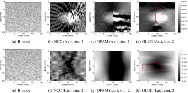
Figure 2.3: Field II and FEM simulation results. A vertical slippage exists in the motion field at the middle of the image. (a) is the first ultrasound image. (b) to (d) are the axial strain images. (e) is the second ultrasound image. (f) to (h) are the lateral strain images. Target and background windows used for CNR calculation of the GLUE results are shown in red. The SNR is calculated for the background window.
significantly outperforms DPAM and NCC in both reducing noise and improving contrast.
In the second simulation (Figure 2.3), we consider tissue slippage which might happen in real world, e.g. at the boundary of different organs such as prostate and rectum (Hoogeman, van Herk, de Bois, & Lebesque, 2005) or for lesions that are not connected to the surrounding tissue. In this experiment, the ultrasound image related to pre-compression is the same as before, whereas a vertical slippage occurs in the second image. The average axial strains to the left and right of the slippage line are respectively1%and2%. The strain images generated using cross correlation, DPAM and GLUE are depicted in (b), (c) and (d) for axial strain and (f), (g) and (h) for lateral strain respectively. As one can see, NCC and DPAM fail in this situation while GLUE accurately computes TDE despite the large discontinuity in the underlying deformation field.
The corresponding SNR and CNR values are measured for both simulation experiments. CNR values are calculated between the target (tumor) and background (outside the target) windows each of size 5 mm×5 mm and 3 mm×3 mm respectively, and are provided in Table 2.1 and Table 2.2. SNR values are also shown in the table, which are calculated for the background windows. GLUE
provides substantially higher SNR and CNR values compared to both NCC and DPAM.
Table 2.1: The SNR and CNR values of the simulation experiment. Target windows (5mm X 5mm) and background windows (3mm X 3mm) used for CNR calculation are shown in Figure 2.2. The SNR is calculated in the background window. Maximum values are in bold font.
SNR CNR
Experiment 1 Axial Lateral Axial Lateral
NCC 2.14 0.52 4.94 7.69
DPAM 5.29 4.50 14.62 10.87
GLUE 44.63 4.61 26.31 11.03
Table 2.2: The SNR and CNR values of the simulation experiment. Target windows (5mm X 5mm) and background windows (3mm X 3mm) used for CNR calculation are shown in Figure 2.3. The SNR is calculated in the background window.
SNR CNR
Experiment 2 Axial Lateral Axial Lateral
NCC Fails Fails Fails Fails
DPAM Fails Fails Fails Fails
GLUE 43.70 4.41 17.45 6.72
2.3.2 Phantom Results
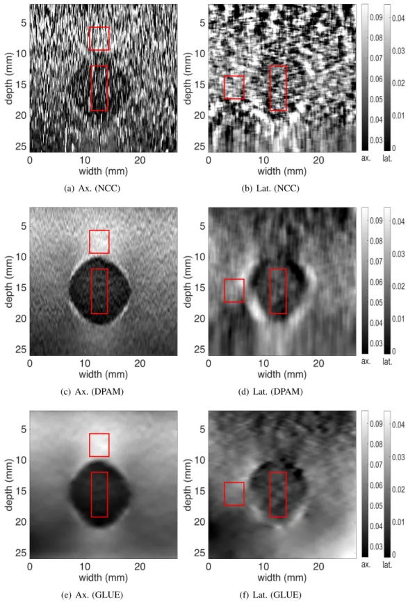
For experimental evaluation, RF data is acquired from a CIRS elastography phantom (Norfolk, VA) using an Antares Siemens system (Issaquah, WA) at the center frequency of 6.67 MHz with a VF10-5 linear array at a sampling rate of 40 MHz. The results of NCC, DPAM and GLUE methods are shown in Figure 2.4, along with the target and background windows used for SNR and CNR calculation. SNR is only calculated for the background window. The results are summarized in Table 2.3. Again, GLUE substantially improves both SNR and CNR in both axial and lateral strain images.
2.3.3 In-vivo Results
TheIn-vivodata is acquired from four patients undergoing open surgical radiofrequency thermal ablation for primary or secondary liver cancers. This data is collected as follows at Johns Hopkins
(a) Ax. (NCC) (b) Lat. (NCC)
(c) Ax. (DPAM) (d) Lat. (DPAM)
(e) Ax. (GLUE) (f) Lat. (GLUE)
Figure 2.4: Results of the phantom experiment. Axial and lateral strain images as well as the target and background windows (in red) for calculation of SNR and CNR are shown (see Table 2.3 for results). The hard lesion is spherical and has a diameter of 1 cm. The axial and lateral strain scales
Table 2.3: The SNR and CNR of the strain images of the experimental phantom. Target and back-ground windows used for CNR calculation are shown in Figure 2.4. The SNR is calculated for the background window. Maximum values are in bold font.
SNR CNR
Axial Lateral Axial Lateral
NCC 2.20 3.60 1.07 0.39
DPAM 26.21 4.77 16.01 3.25
GLUE 29.85 7.22 18.21 4.09
Table 2.4: The SNR and CNR values of the strain images of thein-vivodata in Figure 2.5. The SNR is calculated for the background window of size 6 mm×6 mm. Maximum values are in bold font.
SNR CNR
DPAM GLUE DPAM GLUE
P1 7.94 56.21 3.73 13.64 P2 3.34 13.04 1.46 12.42 P3 4.47 23.29 5.45 20.14 P4 3.22 10.11 3.60 6.62 average 4.74 25.66 3.56 13.20 improv.% - 441 - 271
Hospital: for the first patient, ultrasound RF data is acquired only after ablation. For the second, third, and fourth patients, ultrasound RF data is collected both before and after ablation. Data collection from the tumour involved holding the probe is hard-to-reach locations and angles, which lead to unwanted out-of-plane motions of the probe. In addition, microbubbles and high temperature gradients created by the ablation process add noise in the the RF data. Furthermore, the pulsation of hepatic vessels create complicated deformation fields. Therefore, the pre- and post-compression images suffer from high levels of decorrelation. Traditional NCC failed to estimate the displacement field, and therefore, we only show GLUE and DPAM results in this data.
Figure 2.5 shows B-mode scans, strain images and computed tomography (CT) scans obtained after RF ablation in all four patients. Note that the extent of the ablation is almost completely invisible in B-mode images. The coagulated tissue is clearly visible in strain images, and is marked with red arrows. The CNR values of the ablation lesion are calculated between the target (inside the ablation lesion) and background (outside the target) windows, each of size 6 mm×6 mm. The SNR
(a) B-mode patient 1 (b) DPAM (c) GLUE (d) CT patient 1
(e) B-mode patient 2 (f) DPAM (g) GLUE (h) CT patient 2
(i) B-mode patient 3 (j) DPAM (k) GLUE (l) CT patient 3
(m) B-mode patient 4 (n) DPAM (o) GLUE (p) CT patient 4
Figure 2.5:In-vivoimages of the ablation lesion acquired after ablation of liver tumours. Each row corresponds to one patient. The first column shows ultrasound images, and the second and third columns respectively show the results of DPAM and GLUE. The ablation lesion is marked with red arrows, and is clearly visible in strain images. CT images with the delineated ablation lesions are shown in the right column.
Table 2.5: The SNR and CNR of the strain images of thein-vivodata in Figures 2.6 and 2.7. The CNR calculated for the target and background window each of size 6mm ×6mm. The SNR is calculated for the background window. Maximum values are in bold font.
SNR CNR
DPAM GLUE DPAM GLUE
P2 12.52 17.71 11.27 13.72 P3 8.39 30.15 4.32 12.92 P4 (US 1&2) 16.68 23.23 2.19 13.29 P4 (US 3&4) 9.97 26.21 1.38 14.03 average 11.89 24.32 4.79 13.49 improv.% - 105 - 182
values are calculated for the background windows. Table 2.4 shows that we obtain approximately 5-fold and 4-fold improvements in SNR and CNR respectively by utilizing GLUE method instead of DPAM. The ablation lesion in strain images corresponds well to the post-operative CT images shown in the right column.
Figure 2.6 and 2.7 show pre-ablation results obtained by DPAM and GLUE in second, third and fourth patients. In Figure 2.6, the tumors are marked with red arrows, and are hardly visible in the B-mode images in (a) and (d). The strain images provide a significantly improved contrast between the tumor and healthy tissue. CNR values are calculated between target (inside the tumor) and background (outside the target) windows, each of size 6 mm×6 mm. The SNR values are calculated for the background windows (Table 2.5). Again, we see large improvements with GLUE as a result of utilizing all the data in the RF frames.
Figure 2.7 shows the B-mode, strain, and CT images of Patient 4. All images are obtained before ablation. In (a), the tumor is not visible in the B-mode image. A and B are veins which compress easily due to their low pressure. In contrast, C, D (Arteries) and E (middle hepatic vein) pulsate with the heart beat and may have low or high pressure. The probe motion and variations in the diameter is shown in graph (d). Two ultrasound images US 1 and US 2 (see part (d)) are obtained while the vein diameter variation and probe motion are in the same direction due to high blood pressure. Another pair of ultrasound images, US 3 and US 4, are acquired at low blood pressure when they are pointing to the opposite side in graph (d). Thus, we acquired two paired ultrasound frames at two different phases of the heart beat. The result of DPAM and GLUE using US 1 and 2 are shown
(a) B-mode (b) DPAM (c) GLUE
(d) B-mode (e) DPAM (f) GLUE
Figure 2.6: B-mode and strain images of the patient data before ablation. First and second rows respectively correspond to patients 2 and 3. The red arrows point to the tumours. The strain images provide a substantially improved visualization of the tumours compared to the B-mode ultrasound images.
in (b) and (e) respectively. US 3 and US 4 are used to obtain DPAM and GLUE strain images in (c) and (f). It is very interesting to compare the middle hepatic vein (marked as E in (a)) in strain images in the second and third columns: E looks hard in the second column, and soft in the third column. The reason lies in large pulsation of the middle hepatic vein due to heart beats. CT scans corresponding to two different phases of the heart beat are depicted in (g) and (h). Here, A to D mark the same anatomy as (a).
Table 2.5 summarizes the SNR and CNR values of patients 2 to 4. Average values for DPAM and GLUE are shown in the fifth row. GLUE outperforms DPAM by approximately 2-fold and 3-fold improvements in SNR and CNR values.
(a) B-mode (b) DPAM (US 1&2) (c) DPAM (US 3&4)
(d) probe motion (e) GLUE (US 1&2) (f) GLUE (US 3&4)
(g) arterial phase CT (h) venous phase CT
Figure 2.7: B-mode and strain images of patient 4 before ablation. (a) shows B-mode image, and (b) and (c) show the strain images from the DPAM method using US 1 and 2 frames (for b) and US 3 and 4 frames (for c). (d) shows the motion of the probe and the variation in the diameter of the arteries due to the heart beat. (e) and (f) show results of the GLUE method. (g) is the arterial phase and (h) is the venous phase contrast CT images. The tumor is marked with red arrows in (b), (c), (e), and (f).
2.4
Discussion
Incorporating the prior information of displacement continuity generally improves the TDE. Window-based methods enforce continuity in a small window, DPAM utilizes continuity in a single RF-line, and GLUE utilizes displacement continuity throughout the image. This is a reason for the improvement from window-based methods to DPAM to GLUE. However, there is also a disadvan-tage of using prior information, which is rooted in the bias-variance trade-off (Geman, Bienenstock, & Doursat, 1992; Walker & Trahey, 1995). The prior information decreases the variance, but it increases the bias. The increase in the bias can lead to strain images with lower contrast. Neverthe-less, the substantial improvement in the CNR shows that GLUE strikes a balance between bias and variance.
In order to image some of the tumors during the intervention, the ultrasound probe had to be held at difficult angles, which lead to unwanted out-of-plane motion of the probe during the palpation. Furthermore, ablation creates microbubbles and high temperature gradients, which add high levels of noise to the RF data. Therefore, the pre- and post-compression images suffer from high decor-relation. An advantage of DPAM and GLUE lies within the simultaneous displacement estimation of several samples and exploitation of the continuity prior. As such, both of these methods generate displacement fields from such noisy data, whereas traditional window-based methods calculate the displacement of each window independently and can fail for decorrelated windows. An example of the output of the traditional NCC-based TDE method on this liver data is shown in (Kuzmin et al., 2015).
The regularization term in the GLUE cost function enforces displacement continuity. The strain field is the spatial derivative of the displacement field, and as such, is piecewise continuous in theory (i.e. strain can be discontinuous). This is in fact desired since the strain field can be discontinuous in the boundary between two different types of tissue. In practice, however, large kernels are com-monly used for performing the spatial gradient operation to alleviate noise amplification of the derivative operator. This large kernel guarantees smooth strain fields, but has the disadvantage of blurring the boundary of two different types of tissue. We have proposed Kalman filter (Rivaz et al., 2011) and bilateral filter (Khodadadi, Aghdam, & Rivaz, 2015) to generate piecewise continuous
strain fields that are sharp at the boundary of two different tissue types but are smooth within each type of tissue.
2.5
Conclusion
In this chapter, we introduced GLUE, a novel technique for calculating both axial and lateral dis-placement fields between two frames of RF data. We estimated the disdis-placement field of the entire image simultaneously, which led to substantial improvement over previous work. An unoptimized implementation of the proposed method in MATLAB takes only0.7sec on a typical CPU. There-fore, our technique is highly suitable for implementation in commercial ultrasound systems. An implementation of GLUE is publicly available at https://users.encs.concordia.ca/ ˜hrivaz/Ultrasound Elastography/. In the next chapter, we propose an efficient method
Chapter 3
Efficient Estimation of Tissue
Displacement Using an Affine
Transformation Model
3.1
Introduction
In this chapter, we propose a novel technique for efficient and robust estimation of the initial displacement field. The initial estimation of the GLUE framework is performed using DP, which is computationally expensive. We model tissue deformation using a 2D affine transformation to calculate an approximate initial displacement. We call our method ATME: Affine Transformation Model Elastography. Since 2D affine transformation has only six degrees of freedom (DOF), it can be efficiently estimated by minimizing a quadratic error measure. Afterward, regularized global cost function is optimized by using initial displacement fields obtained from the previous step. We convert the optimization problem to a set of equations, which entails solving a sparse linear system, and as such, is computationally efficient.
The importance of the affine transformation model is twofold. First, there are only six parame-ters to estimate for the total RF frame, which is computationally efficient and suitable for real-time
Figure 3.1: Displacement field between a pair of ultrasound images in a uniform tissue.
implementation. Second, the prior information that tissue deformation is relatively planar is uti-lized. Therefore, this method is able to estimate tissue displacements in the presence of large noise. It is also robust to signal decorrelation by exploiting the prior information that tissue deformation is smooth. This method can be applied to a range of elastography imaging techniques including freehand palpation, wherein tissue is deformed gently using a hand-held ultrasound probe.
The rest of the chapter is organized as follows. We first introduce ATME, and derive the equa-tions for estimation of TDE from RF data. We then show that ATME outperforms previous work using simulation experiments. We then collect RF data fromin-vivo patellar tendon and medial collateral ligament (MCL) of healthy volunteers, and conclude the chapter by showing that ATME can recover tendon and MCL motion in such challenging data.
3.2
Methods
Let I1(i, j) and I2(i, j) be two ultrasound RF frames acquired before and after some tissue deformation, and i and j respectively be samples in the axial and lateral directions. The main idea is to enforce an affine displacement field between the two ultrasound images, such that an approximate initial displacement field can be calculated. This initial displacement field will then be utilized in a cost function that incorporates similarity of RF data intensity, as well as prior information of displacement continuity. Since the initial displacement field is affine, its estimation will be both fast and robust.
field, assume that the tissue is homogenous and isotropic. In such medium, free-hand palpation ultrasound elastography generates a planar deformation field for both axial and lateral displacements (Fig. 3.1). This planar deformation can be simply formulated using affine transformation, which has only 6 DOF. As such, estimation of this transformation is very efficient. Furthermore, there is a smaller chance of getting trapped in a local minimum. Real tissue is neither homogenous nor isotropic, and therefore, actual deformation is not planar. Therefore, this planar deformation can only be used as an approximation of the true underlying displacement. We use a hierarchal affine transformation model similar to the technique proposed in Ref. (Bergen, Anandan, Hanna, & Hingorani, 1992):
a(x, y) =g1+g2x+g3y l(x, y) =g4+g5x+g6y
(15)
whereaandlare axial and lateral displacements of a pixel at(x, y)location. The affine parameter gi can be obtained by minimizing an error functionE(δg)with respect to an incremental estimate gthrough an iterative procedure. To formulateE, let , and denote the current estimate of the affine parameter, axial and lateral displacements, respectively. The error functionE(δg)is defined as:
E(δg) = n X y=1 m X x=1 (∆I+ (∇I)TXδg)2 (16)
where∆I =I2(x, y)−I1(x−ak, y−lk), and∇I is the gradient ofI1. The matrixXis defined as: D= 1 x y 0 0 0 0 0 0 1 x y (17)
To simplify the notation of single pixel displacement, we simplifya(x, y)toai,j andl(x, y)to li,j. Once the initial displacement field is estimated, it can be utilized in the next step. The cost function with the summation on all image pixels is defined as:
(a) Axial displacement (Ground truth) (b) Lateral Displacement (Ground truth)
(c) Axial displacement (ATME) (d) Lateral displacement (ATME)
Figure 3.2: Field II and finite element simulation results. (a) and (b) show the axial and lateral ground truth displacement images of the simulation experiment. (c) and (d) are the corresponding axial and lateral displacement fields obtained from ATME.
C(∆a1,1,· · · ,∆am,n,∆l1,1,· · · ,∆lm,n) = n X j=1 m X i=1
{[I1(i, j)−I2(i+ai,j, j+li,j)−∆ai,jI2,a0 −∆li,jI2,l0 ]2
+α1(ai,j+ ∆ai,j−ai−1,j−∆ai−1,j)2+β1(li,j+ ∆li,j−li−1,j−∆li−1,j)2
+α2(ai,j+ ∆ai,j−ai,j−1−∆ai,j−1)2+β2(li,j+ ∆li,j−li,j−1−∆li,j−1)2}.
(18)
whereαandβ are regularization terms for axial and lateral displacements respectively. By mini-mizing the cost function using the initial guess(ai,j, li,j), the sub-sample axial and lateral displace-ments(∆ai,j,∆li,j)for the total image are calculated. The initial displacements(ai,j, li,j)provided through the previous step are added to the subsample displacements. This presents us the final lat-eral and axial displacements i.e.(ai,j+∆ai,j, li,j+∆li,j). Once the displacement field is estimated, its spatial gradient is calculated to obtain the strain image.
3.3
Experiments and Results
We tested our proposed method on acquired data from simulation and clinical trials. In this section, we also present results of clinical trials using a previous work, DPAM (Rivaz et al., 2011), to compare with ATME. Estimation of lateral displacement is significantly more difficult mainly due to the poor resolution of ultrasound images in this direction, thereby limiting previous work to only calculate axial strain images. Simultaneous estimation of the displacement filed for the entire image, however, allows us to substantially improve the quality of both axial and lateral displacements.
3.3.1 Simulation Experiments
Field II software (Jensen, 1996) is used to simulate ultrasound images. The phantom is homoge-nous and isotropic with a Poisson ratio ofν = 0.49. A uniform axial force profile is applied to the top of the phantom to generate 6% axial strain. More than 12 scatterers are randomly distributed in each cubic millimeter of the phantom to generate fully developed speckles. Further details of the data acquisition are available in Ref. (Rivaz et al., 2011). The Axial and lateral ground truth displacements and also the ones obtained by ATME are shown in Fig. 3.2. Note that the tissue is homogenous, and therefore, the deformation is assumed to be planar.
Table 3.1: The SNR and CNR of the strain images of Fig. 3.5. Maximum values are in bold font.
SNR CNR
Experiment DPAM ATME DPAM ATME
Patellar tendon flexion (distal portion) 4.77 10.06 5.46 11.98
Patellar tendon flexion (proximal portion) 6.41 9.17 3.51 3.24
MCL pure valgus 0.7 4.17 1.26 2.16
MCL pure valgus 3.20 6.59 6.28 10.70
Average 3.77 7.50 4.13 7.02
3.3.2 in-vivoExperiments
Ethics approval was obtained at both McGill University Health Centre (MUHC) and Concordia University to collect ultrasound images of human subjects. Valgus stress was applied to the knee, and ultrasound data of the MCL was collected during the stress. In the second set of experiments,
(a) Axial Displacement (b) Lateral Displacement
(c) B-mode (d) Axial Strain
(e) Strain directions
Figure 3.3: Distal tendon motion during force flexion experiment. (a) and (b) show axial and lateral displacements. (c) is the B-mode image and red arrows represent the strain directions in the tendon. (d) and (e) depict the axial strain and magnified strain directions respectively.
the subject freely flexed their knee, and ultrasound data was collected from the patellar tendon, and all subjects signed a consent form. Valgus stress and knee flexion generates strain in the MCL and patellar tendon respectively, and we examined whether this strain can be measured using ATME. RF data was collected with an Alpinion ultrasound machine (Bothell, WA) with an L3-12 linear transducer at the centre frequency of 11MHz and sampling frequency of 40MHz. Ligaments and tendons play a significant role in musculoskeletal (MSK) biomechanics, and constantly change due to factors such as aging, injury, disease or exercise. Conventional B-mode ultrasonography has been widely used as a first line diagnostic modality for superficial structures such as the patellar tendon and MCL. Strain imaging captures dynamics of tissue motion and captures deformations of the patellar tendon and MCL, which are not directly available in B-mode images. These deforma-tion patterns reveal mechanical properties of tendon and therefore may reveal important pathology otherwise hidden in the B-mode scans (Chimenti et al., 2016).
Fig. 3.3(a) and (b) show the displacement of the distal tendon (lower portion of patellar tendon connected to tibia) during in-vivoforced flexion. The B-mode image is demonstrated in (c). Red arrows represent strain directions and their relative amplitudes in a region of interest. The patellar tendon is marked with blue arrows. The axial strain is shown in (d) wherein we can clearly distin-guish the boundaries of tendon from rest of the tissue. The strain arrows in (c) are magnified and depicted in (e) for better visualization. The results in (e) are in good agreement with our expecta-tion of strain in the patellar tendon: the strain is relatively high close to the patella (the hyperechoic dome-shaped structure in bottom left of (c) with the shadow underneath), where it is getting pulled by the joint. The strain is also tensile (arrows pointing to the left) at the top, and compressive at the bottom (arrows pointing to the right) in (e), as we expect from a bent structure (i.e. the patellar tendon).
Fig. 3.4(a) and (b) demonstrate the motion fields of MCL when the pure valgus stress is applied on the knee. (c) and (d) show the B-mode and strain images respectively. MCL is marked with blue arrows in (c). Strain directions which are shown with red arrows in (c) are enlarged in (e). Again, the strain field corresponds well with what we expect: high tension at the top where the extension is maximum in the bent MCL.
(a) Axial Displacement (b) Lateral Displacement
(c) B-mode (d) Axial Strain
(e) Strain directions
Figure 3.4: MCL during pure valgus stress experiment. (a) and (b) show axial and lateral displace-ments. (c) is the B-mode image and red arrows represent the strain directions in the MCL. (d) and (e) depict the axial strain and magnified strain directions respectively.
(a) B-mode (b) DPAM strain (axial) (c) ATME strain (axial)
(d) B-mode (e) DPAM strain (axial) (f) ATME strain (axial)
(g) B-mode (h) DPAM strain (axial) (i) ATME strain (axial)
(j) B-mode (k) DPAM strain (axial) (l) ATME strain (axial)
Figure 3.5: comparison between ATME and DPAM methods. (a), (b), and (c) show distal area of patellar tendon during force flexion experiment. (d), (e), and (f) are proximal region of patellar tendon. (g)-(l) are B-mode and strain images of MCL during pure valgus stress experiment.
MCL during flexion. For the purposes of comparison, strain images were also calculated using a previous work, DPAM (Rivaz et al., 2011). In the first row, the distal portion of the knee is shown while the forced flexion is applied to patellar tendon. In the second row, the same experiment is practiced but the proximal portion of the knee is depicted here. Third and forth rows show the MCL when pure valgus stress is placed on the knee. The valgus stress test is performed with the knee at
30◦ of flexion.
The unitless metrics signal to noise ratio (SNR) and contrast to noise ratio (CNR) are used to quantitatively compare the results (Ophir et al., 1999):
CNR = C N = s 2( ¯sb−s¯t)2 σ2 b +σ2t , SNR = s¯ σ (19)
wheres¯t ands¯b are the spatial strain average of the target and background, andσt2 andσ2b are the spatial strain variance of the target and background, ands¯andσare the spatial average and variance of a window in the strain image respectively. The corresponding SNR and CNR values are measured for both DPAM and ATME methods. CNR values are calculated between the target (tendon) and background (outside the target) windows each of size 50 samples×50 samples, and are provided in Table 3.1. SNR values are also shown in the table, which are calculated for the background windows. ATME provides substantially higher SNR and CNR values compared to DPAM.
3.4
Conclusion
In this chapter, we introduced a novel technique to calculate both axial and lateral displacement fields between two frames of RF data based on affine transformation prior. Optimization of the main global cost function involves solving a sparse linear system which can be solved in real time and provide the displacement field of the entire image simultaneously. We further applied strain imag-ing to patellar tendon and MCL, and showed that our proposed technique can be used to predict displacement and strain fields in these tissues. Future work will utilize these dynamical measure-ments of the patellar tendon and MCL to both improve diagnosis and manage treatment. In the next chapter, we summarize the contributions of this thesis and provide directions for future work.
Chapter 4
Conclusion and Future Work
4.1
Conclusion
Ultrasound elastography has numerous clinical applications in monitoring and treatment of in-juries and diseases because pathology usually affects tissue elasticity. It is considered as a non-invasive, convenient, and real-time imaging modality that has been successfully translated from benchside to bedside. In this thesis, we focused on quasi-static elastography wherein tissue de-formation is slow and is generated by slowly palpating the tissue with the hand-held ultrasound probe. Numerous techniques have been developed to calculate time-delay estimation between pre-and post-compression images, but ultrasound data is highly noisy pre-and previous work suffers from inaccurate displacement estimates.
In this thesis, we first introduced GLUE, a novel technique for calculating both axial and lateral displacement fields between two frames of RF data. Optimization of the main global cost function involves solving a sparse linear system which can be solved in real time. We estimated the displace-ment field of the entire image simultaneously, which led to substantial improvedisplace-ment over state of the art. Our implementation of GLUE in MATLAB takes only0.7sec on a typical CPU. Therefore, our technique is highly suitable for implementation in commercial ultrasound systems. We have also made an implementation of GLUE available online, which will facilitate knowledge transfer and will amplify the impact of this work.