Dynamic interest rate and credit risk models

(1)

Dynamic Interest Rate and

Credit Risk Models

Adam Saeed Iqbal

Imperial College Business School,

Imperial College London

This thesis is submitted in partial fulfillment of the

requirements for the degree of Doctor of Philosophy

(2)

Declaration of Originality

I declare that the research presented in this thesis is my own and that all else is appro-priately referenced.

(3)

To my parents

with

(4)

Acknowledgements

I thank William Perraudin for his supervision, for his insightful feedback and for allowing me the freedom to pursue my academic interests.

I thank Lara Cathcart for her general comments on my research and, in particular, for her encouragement and guidance towards completing this thesis.

I am grateful to Julie Paranics for her efforts on the administrative side in helping me return to research following an unexpected interruption to studies.

Finally, I thank my PhD colleagues, Leo Evans, Filip Zikes, Ewan Mackie and Robert Metcalfe, for many interesting discussions about research and for their friendship.

(5)

Thesis Abstract

This thesis studies the pricing of Treasury bonds, the pricing of corporate bonds and the modelling of portfolios of defaultable debt. By drawing on the related literature, Chapter 1 provides economic background and motivation for the study of each of these topics.

Chapter 2 studies the use of Gaussian affine dynamic term structure models (GDTSMs) for forming forecasts of Treasury yields and conditional decompositions of the yield curve into expectation and risk premium components. Specifically, it proposes market prices of risk that can generate bond price time series that are consistent with the important empirical result of Cochrane and Piazzesi (2005), that a linear combination of forward rates can forecast excess returns to bonds. Since the GDTSM here falls into the essentially affine class (Duffee (2002)), it is analytically tractable.

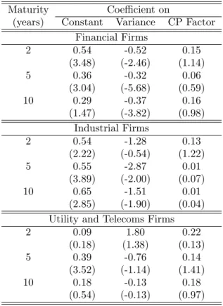
Chapter 3 studies conditional risk premia in a commonly applied default intensity based model for pricing corporate bonds. Here, I refer to such models as completely affine defaultable dynamic term structure models (DDTSMs). There are two main contribu-tions. First, I show that completely affine DDTSMs imply that the compensation for the risk associated with shocks to default intensities (the credit spread risk premium) is related to the volatility of default intensities. Second, I run regressions to show that this relationship holds in a set of corporate bond data.

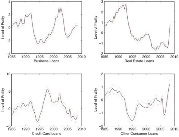
Finally, Chapter 4 proposes a new dynamic model for default rates in large debt port-folios. The model is similar in principle to Duffie, Saita, and Wang (2007) and Duffie, Eckner, Horel, and Saita (2009) in that the default intensity depends on the observed macroeconomic state and unobserved frailty variables. However, the model is designed for use with more commonly available aggregate, rather than individual, default data. Fitting the model to aggregate charge-off rates in US corporate, real-estate and non-mortgage retail sectors, it is found that interest rates, industrial production and unem-ployment rates have quantitatively plausible effects on aggregate default rates.

(6)

List of Abbreviations

CAPM Capital Asset Pricing Model.

CCAPM Consumption Based Capital Asset Pricing Model.

CDO Collateralised Debt Obligation.

CDS Credit Default Swap.

CPI Consumer Price Index.

DTSM Dynamic Term Structure Model.

DDTSM Defaultable Dynamic Term Structure Model.

GDP Gross Domestic Product.

HMI Housing Market Index.

ICAPM Intertemporal Capital Asset Pricing Model.

IID Independently Identically Distributed.

IP Industrial Production.

LEH Local Expectations Hypothesis.

ML Maximum Likelihood.

MLE Maximum Likelihood Estimate.

MPR Market Price of Risk.

MSE Mean Squared (Forecast) Error.

(10)

OLS Ordinary Least Squares.

SDF Stochastic Discount Factor.

VAR(n) Vector Autoregression of Order n.

(11)

Chapter 1

Interest Rate and Credit Risk

Modelling

This thesis contributes to the literature on dynamic asset pricing applied to fixed income securities. The contributions are in three closely related areas: the pricing of Treasury bonds, the pricing of defaultable corporate bonds and the modelling of portfolios of defaultable debt. The purpose of this introductory chapter is to provide motivation and to describe background literature for the study of the above mentioned topics and to explain the close relationships that exist between them.

1.1 Pricing Treasury Bonds

1.1.1 Why Study Treasury Bond Returns?

One may ask, why should we study risk premia in Treasury bond returns? In this subsection, I provide several reasons organised according to their relevance to different participants in the economy: households, firms and government. This is not intended to be an exhaustive list, but it explains the substantial past and present research effort devoted to understanding the shape of the yield curve and its co-movement over time.

Households - Consumers and Investors

Treasury bonds, like stocks and derivatives, are assets that expose their holders to eco-nomic risks. From the perspective of an investor, the reason for studying bond prices is therefore the same as that for studying the pricing of any asset: the statistical proper-ties of bond returns will influence the investor’s optimal consumption-portfolio decision. Moreover, since bond pricing is the basic building block of all asset pricing, the study

(12)

of bond returns is of particular importance. The remainder of this subsection explains these ideas.

As the availability of data on bond returns has increased, so has our understanding of their statistical properties. This has implications for optimal consumption-portfolio decisions, as I now describe.

The classic theory of bond returns is the expectations hypothesis. It says that expected excess returns to Treasury bonds of all maturities over bills equal a fixed constant12. If the expectations hypothesis were true, then the conditional expected excess return to bonds at any time is equal to its unconditional counterpart. Under the portfolio rules of the one-period static Capital Asset Pricing Model (CAPM) (Sharpe (1964), Lintner (1965, 1965a), Mossin (1966)) or a standard continuous time optimal consumption-portfolio model (Merton (1969, 1971)), the consumption-portfolio weight assigned to a particular asset depends on its expected excess return (as well as other properties such as the co-variance matrix of all assets and risk aversion parameters). The expectations hypothesis tells us that, provided that the other assumptions that underly these portfolio models are appropriate, unconditional bond returns may be used here to address the optimal consumption-portfolio problem.

However, it is well known that the expectations hypothesis is not supported by the data and expected excess returns to bonds are time-varying and forecastable using forward rates or yield spreads (Fama and Bliss (1987), Campbell and Shiller (1991)). More recently, Cochrane and Piazzesi (2005, 2008) have found empirical evidence that a single factor, a linear combination of five forward rates, is able to forecast expected excess returns to bonds of all maturities.

The recent empirical evidence suggests that the forward rates that form the above men-tioned return forecasting factor are state variables that are required to describe the conditional distribution of bond returns. In other words, there are shifts in the invest-ment opportunity set. This means that an Intertemporal CAPM (ICAPM) (Merton (1973a)) is required to address the optimal consumption-portfolio problem. The search for state variables is an unfinished task and it provides motivation to study bond prices 1_{To be precise, the expectations hypothesis says that expected log (rather than continuously}

com-pounded) holding period returns across maturities are equal to a constant. The difference is small. For example, if annual returns are distributed as lnR ∼ N(µ, σ2) then E[R] = eµ+

1

2σ2_{. If} _µ _{= 0}_._{1 and} σ= 0.1 then 1

2σ

2_{= 0}_._{005 which is very small compared with}_µ_{, but not zero.} 2

(13)

and, in particular, conditional bond returns. In Chapter 2, I construct a term structure model that is motivated by this recent empirical evidence.

More generally, since investors optimise their portfolios across all assets, a more funda-mental reason to focus on Treasury bonds in particular is that bond pricing is the basic building block of all asset pricing. Any asset can be thought of as a bond plus cash flow risk. As a result, being able to price a bond is necessary to price any asset and an understanding of the statistical properties of bond returns is necessary to understand the statistical properties of returns to any asset. This point can be seen as follows. The absence of arbitrage implies the existence of a stochastic discount factor (SDF),π, that prices all traded assets (Harrison and Kreps (1979)). By the definition of the SDF, the price of any non-dividend paying asset at time t,St, is given by

St=Et πT πt ST for allT > t, (1.1)

where Et denotes the time t conditional expectation. We can apply this equation to

price bonds. A zero-coupon bond that matures at time T has, by definition, a price of 1 at time T. LettingPt(T) denote the time tprice of a zero-coupon bond that matures

at timeT, an application of (1.1) reveals that Pt(T) =Et πT πt . (1.2)

Next, by defining a random variablet,T by

t,T ≡ST −Et[ST]

and substituting this and the result in (1.2) into (1.1) we can rewrite the asset pricing equation as St=Pt(T)Et[ST] +Et πT πt t,T for all T > t. (1.3) This equation says that the price of any asset is simply the price ofEt[ST] zero-coupon

bonds that mature at time T plus a cash flow risk term. The above arguments make clear that, of all assets, it is particularly important that we understand the pricing of bonds. A similar result holds for dividend paying assets.

The term structure literature is extensive. Most of this literature emphasises risk-adjusted probabilities and does not address the issue of specifying drifts and market

(14)

prices of risk. That is, authors have proposed only the risk-adjusted dynamics for the short rate and then calibrated the parameters to the cross section of bond prices. The one-factor models of Ho and Lee (1986), Black, Derman, and Toy (1990), Black and Karasinski (1991) and Hull and White (1990, 1993) are examples of such an approach, and numerous authors (too many to list here) have calibrated models in which the risk-adjusted dynamics of the short rate follow the stochastic process suggested in Va-sicek (1977), Cox, Ingersoll, and Ross (1985) or a multifactor generalisation of these as described in Duffie and Kan (1996).

The approach of specifying only risk-adjusted probabilities only may be appropriate for applications such as pricing derivatives on bonds relative to the bond itself, where accurate volatility modelling is the most important concern. It is also suitable for con-structing a smooth yield curve across all bond maturities to price bonds of non-traded maturities when the bond prices of only a subset of maturities are known (Section 1.1.2 below discusses cross sectional bond pricing further). However, this literature does not address empirical facts about expected excess returns to bonds and it is therefore not useful for studying the portfolio selection problems faced by households.

More recently, several authors have begun to specify models that attempt to fit both the cross section of bond prices and also the empirical facts about the temporal behavior of bond returns. Models that simultaneously attempt to understand the shape of the yield curve (the cross section of bond prices) and its co-movement over time are com-monly known in the literature as dynamic term structure models (DTSMs). Prominent contributions in this area are Duffee (2002), Dai and Singleton (2002) and Duarte (2004). DTSMs is an important field of current research. The research presented in Chapter 2 of this thesis is a contribution in this direction. Specifically, it takes the arbitrage free modelling framework proposed by Duffee (2002) and imposes restrictions on market prices of risk so that the model is able to generate return forecasting equations that are, in principle, consistent with the empirical results of Cochrane and Piazzesi (2005). Based on the recent insights presented in Joslin, Singleton, and Zhu (2010) relating to Gaussian affine DTSMs, the model is tested by comparing its out-of-sample yield forecasting ability with a more general nesting model.

Firms

The observed real yield curve and an understanding of conditional risk premia in bond returns can shed light on firms’ investment decisions in that, together, they can provide

(15)

conditional forecasts for future levels of consumption at multiple future times. If con-sumption is forecast to increase, then firms must be investing to increase their inventories in anticipation of higher future consumer spending at the time points suggested by the real yield curve. It is not surprising that asset prices can provide such forecasts. After all, it is through trading in financial markets that consumers are able to reflect their marginal rates of substitution across time. These ideas can be understood in the frame-work of a conditional macroeconomic asset pricing model/consumption based capital asset pricing model (CCAPM) as follows.

Suppose that at timetthe objective of a representative economic agent is to maximise his or her long term expected utility by choosing a number, ξ, of the n-period zero-coupon bond to purchase. Assuming a time separable form for the agent’s utility function, this problem can be written as

max {ξ} Et U({ct+j}∞j=0) = max {ξ} Et   ∞ X j=0 βju(ct+j)  , such that ct = et−ξPt(t+n), ct+j = et+j, for j= 1, . . . , n−1, n+ 1, . . . ,∞ ct+n = et+n+ξ,

wherect+j andet+j are the timet+jlevels of consumption and endowment respectively,

andU({ct+j}∞j=0) = P∞

j=0βju(ct+j) is the utility function for someimpatienceparameter

β <1. The first order conditions reveal that the n-period real bond yield,Rn_t, is given by Rn_t ≡ 1 Pt(t+n) = 1 Et h βu0(ct+n) u0₍_c t) i. (1.4)

This equation applies once households have implemented their consumption-portfolio choices. A high n-period real bond yield today suggests that, in expectation, u0(ct+n)

will be small relative to u0(ct). For a concave u(·) this means that ct+n is likely to be

large relative to ctand consumption is forecast to rise. Firms may react to this forecast

to ensure that they minimise unplanned changes to their inventories over time. An important question is, given the time t real n-period yield, how much is consumption forecast to rise? The empirical evidence about bond returns suggests that the answer to this question may change over time; it is related to timetconditional risk premia. This can be understood as follows.

(16)

forecasts depends on the form of u0(·)3. In turn, u0(·) depends on the representative agent’s level of risk aversion. For example, in the case of an agent with power utility, u0(c) = c−γ_{, which depends on the risk aversion parameter} _γ_{. The complication is,}

however, that γ may vary over time (perhaps γt is more appropriate notation). Some

evidence supporting the suggestion thatγ varies over time is given below. However, the main implication here is that at times when γ is large, smaller increases in expectations of ct+n relative toctcan deliver higher n-period bond yields relative to times whenγ is

small. In the power utility example, the quantity u0(ct+n) u0₍_c t) = ct+n ct −γ

and so marginal utility growth is more sensitive to consumption growth at larger γ. Therefore, to use yields to forecast future consumption, sinceγ is generally unobserved, one must be able to at least proxy for its temporal variation.

The empirical fact that excess returns to bonds are predictable was discussed in the previous subsection. Further, it is a standard result in a CCAPM with power utility and log normal consumption growth that expected excess returns depend on γ:

Et Pt+1(t+n) Pt(t+n) −R1_t ≈γσt ct+1 ct σt Pt+1(t+n) Pt(t+n) ρt β ct+n ct −γ ,Pt+1(t+n) Pt(t+n) ! . (1.5) Here, the notation σt(·) denotes the conditional standard deviation and ρt(·,·) denotes

the conditional correlation.

Given the above equation, one way of reconciling the predictability of excess returns to bonds with the CCAPM is that γ is time varying. If changing risk aversion is indeed the fundamental source of return predictability then variables such as forward rates, yield spreads and combinations of forward rates that have been used to forecast excess returns to bonds in Fama and Bliss (1987), Campbell and Shiller (1991) and Cochrane and Piazzesi (2005) may be good proxies for the temporal variation inγ. These proxies can be used to help make conditional forecasts of consumption. The research presented in Chapter 2 contributes to our understanding of the relationship between forward rates and the predictability of Treasury bond returns by reconciling this predictability with an arbitrage free (tractable) DTSM.

3_{The term “associated” is used to emphasise that the causality here is not clear; both consumption}

(17)

As an aside, it is noteworthy that, since in principle one can use a CCAPM to price all assets, other asset prices can also be used to forecast consumption. However, this requires knowledge of the asset’s expected dividend (for stocks) or coupon payment (for defaultable bonds) at multiple future dates and the correlation of these dividends and default risky coupons with consumption. Amongst all assets, default-free zero-coupon Treasury bond prices provide perhaps the simplest data with which to forecast future consumption. Indeed, many articles have used the yield curve/bond prices to forecast future real economic activity (Harvey (1988), Estrella and Hardouvelis (1991), Hamilton and Kim (2002), Ang, Piazzesi, and Wei (2006) are some well known examples). Stock and Watson (2003) provide a detailed survey of the literature that has used bond prices as well as the prices of other assets (stocks, gold and others) to forecast economic output.

Governments and Central Banks

The DTSM in Chapter 2 attempts to quantify the size and variation over time of risk premia in Treasury bond returns. These quantities have implications for government debt policy relating to both the timing of debt issuance and to the management of its maturity structure. These ideas can be understood as follows.

Conditional risk premia are relevant for the timing of debt issuance for a government wishing to minimise its actuarial financing costs; the government may wish to avoid issuing debt when risk premia are high. This may be challenging. For instance, some governments use fiscal stimuli in efforts to counter recessions. They must therefore raise finance when recessions are forecast. However, this may be precisely the time when risk premia and therefore the cost of raising debt is highest. Indeed, there is empirical evidence that variables that forecast high excess returns also forecast recessions. The term spread is a well known example of a variable that forecasts excess returns to stocks and bonds and also recessions (Fama and French (1989)). Another example is the index dividend to price ratio, which is found to forecast excess returns in equity indices (Cochrane (1992)). Since most expected cash flow variation in the cross section of firms is idiosyncratic, the variation in the index dividend to price ratio is mostly due to varying expected excess returns (Vuolteenaho (2002)).

The idea that the same variables that forecast excess returns also forecast recessions is intuitive. One may expect risk aversion and hence, by (1.5) above, risk premia to be highest when a recession is forecast; investors may require a larger risk premium to be induced into holding risky assets when their outside income becomes less certain.

(18)

Campbell and Cochrane (1999) present an economic model that captures the idea of a recession premium. A DTSM with market prices of risk specified with sufficient flexibility to capture the time variation in risk premia can allow one to calculate the conditional component of the cost of debt due risk premia and that due to expectations of future interest rates. The research in Chapter 2 is in the direction of finding such a specification. Risk premia are also relevant to a government wishing to choose the maturity structure of its debt in a way that is optimal in terms of cost. The rationale for actively man-aging the maturity structure of public debt is not clear in frictionless markets with no distortionary taxes. The reason is that the Modigliani-Miller theorem (Modigliani and Miller (1958, 1961)) applies. Nevertheless, despite this, the actuarial expected cost to the government for financing its debt can depend on debt maturity. For example, if the term structure of the risk premium to bonds is downward sloping, then, after an adjustment for expectations of future short interest rates, financing using long bonds is actuarially less expensive than financing with short bonds. Campbell, Shiller, and Viceira (2009), for instance, find that long term inflation-indexed bonds are safe assets in that they command a low risk premium and argue that they are therefore a relatively cheap method of debt financing for governments.

Another reason to study risk premia in bond returns relates to stabilisation policy, a public policy often implemented by central banks aimed at manipulating aggregate demand to reduce the severity of short run economic fluctuations. The relevance of bond risk premia here can be understood as follows.

Loosely speaking, in a rational expectations framework, only movements in interest rates (through, for example, monetary action) that are unexpected by households can change their consumption-portfolio decisions. In order to manipulate aggregate demand, therefore, it is useful for the central bank to know households’ conditional expectations of future interest rates. Here, risk premia complicate matters. In general, yields on long maturity bonds are expected values of average future short yields only after adjustment for risk (the strategy of rolling over short bonds is “risky” compared with buying and holding a long bond). In other words, extracting conditional expectations of future interest rates from the yield curve requires a knowledge of conditional risk premia. Chapter 2 is a contribution in this direction.

The above discussion is mainly concerned with the time series behaviour of bond prices. It is important to note that studying the cross section of bond prices is also relevant to stabilisation policy. For example, the central bank is usually able to move the short

(19)

end of the yield curve. In the USA, for instance, the Federal Open Market Committee has in the past used and continues to employ the federal funds rate, the interest rate banks charge one another for overnight loans, as a policy instrument. This can move the short end of the yield curve. However, the main purpose is to shift the aggregate demand curve, but this depends on long term rather than short term yields. For instance, households base their decision on whether to buy or rent a house on long-term mortgage rates and not the federal funds rate. A no-arbitrage model of the yield curve can provide an understanding of the how short yields translate into long yields. This is the topic of the subsection below.

1.1.2 Pricing in the Cross Section

Studying the cross sectional relationships between bond prices is useful for at least three reasons. Two of these were mentioned above: to understand how movements in the short end of the yield curve translate into movements at the long end, and to price derivatives on bonds. A third reason is that the cross sectional relationships between bond prices can be used in separating risk premia from expectations about future short rates; Chapter 2 focusses on this topic. These reasons can be understood as follows. A cross section of bonds of different maturities can be liquidly traded and so the as-sumption that there are no arbitrage opportunities is certainly reasonable. Further, if in addition, the short rate of interest,rt, is assumed to depend on a Markov state vector

Xt, then bond prices can be written as a function ofXt:

Pt(T) =EQt h e− RT t rudu i =f(Xt, t, T;ψ). (1.6)

Here, Q denotes the risk-adjusted probability measure andψdenotes a vector of param-eters that (i) enter the Q dynamics of the stochastic process followed byXtand (ii) that

determine the dependence ofrt on Xt.

First, given the above equation, it is possible to understand how movements in different parts of the yield curve relate to each other. For instance, in the affine framework of Duffie and Kan (1996) each element of Xt is a bond yield of a different maturity. One

can therefore see the affect on yields that are not inXtof changing a yield that is inXt.

Next, given the cross section of bond prices at a given point in time, it is possible to calibrate the parametersψto fit, by some criterion, the observed prices. In other words, it is possible to extract information about the Q dynamics followed byXtfrom the cross

(20)

bonds.

Finally, given the Q dynamics of Xt and information about the time series behaviour

of Xt (the P dynamics), it is possible to calculate risk premia in bond returns. For

example, if the cross section of bond prices reveals an upward sloping yield curve and simultaneously interest rates are forecast to fall then this suggests that risk premia on long maturity bonds are positive.

1.2 Pricing Corporate Bonds

1.2.1 Background

Given the seminal literature on and relating to the pricing of corporate bonds (Black and Scholes (1973), Merton (1973b, 1974)), one may suggest that the corporate bond pricing problem is redundant once the firm itself has been priced. The reason is that this literature models corporate debt as a contingent claim on the firm in a locally complete market and so once the firm has been priced, it is straight forward to price the bond relative to the firm by a no-arbitrage argument. However, under this model the predicted levels of corporate bond spreads are on average substantially lower than those observed empirically (Jones, Mason, and Rosenfeld (1984), Eom, Helwege, and Huang (2004)). This has lead to many extensions to make these frameworks more realistic in their modelling of a firm’s default process. The original models and the subsequent extensions are classified as structural models. Despite the increasing complexity of and increasing realism captured in structural models, the empirical support for them is mixed, as I discuss below.

Structural Models of Corporate Bonds Prices

Among the well known extensions to the above mentioned literature is Geske (1977) who uses compound option modelling methods to price debt at multiple maturities. Longstaff and Schwartz (1995) developed a pricing model with stochastic default-free interest rates and build on the idea first proposed in Black and Cox (1976) that default occurs when the value of assets first pass below an exogenously imposed default boundary. Collin-Durfesne and Goldstein (2001) reflect firms’ behavior by allowing for mean-reverting leverage ratios in addition to stochastic interest rates and an exogenously imposed default boundary. Leland and Toft (1996) extend previous models of optimal default timing and the valuation of debt with taxes and bankruptcy distress costs (Fisher, Heinkel, and Zechner (1989), Leland (1994)) to allow for coupon debt of finite maturity. However, Eom, Helwege, and Huang (2004) have found that, with the exception of Leland and

(21)

Toft (1996), all of the above mentioned extensions under predict level of corporate bond spreads for safer bonds and overpredict spreads on firms with high leverage or volatility. They also find that Leland and Toft (1996) overpredicts spreads on most bonds and particularly so on those with high coupons.

Intensity Based Models of Corporate Bond Prices

Given the above mentioned empirical difficulties associated with structural models, a large proportion of the recent corporate bond modelling literature and the closely related credit default swap (CDS) modelling literature has focussed on another class of models: the intensity based default models that were introduced by Artzner and Delbaen (1990, 1995), Jarrow and Turnbull (1995) and Lando (1998). These are models in which default is said to occur at the first jump time of a conditional Poisson process. That is, loosely speaking, conditional on no default occurring until time t, the probability that the corporate will default in the next small amount of time ∆tis approximatelyλt∆t. λt is

called the default intensity and it can be shown that it is also closely related to the short corporate bond spread. λtcan be allowed to follow a non-negative stochastic process.

Intensity based models have gained popularity for their simplicity, flexibility and ana-lytical tractability. In particular, Duffie and Singleton (1999) provide a framework in which the short rate of interest is “default adjusted” so that corporate bond pricing problems simplify to Treasury bond pricing problems. Under the restriction that the default adjusted short rate of interest is an affine function of a state vector that follows an affine diffusion under the risk adjusted probability measure, the full machinery of Duffie and Kan (1996) that was originally designed for the relative of pricing Treasury bonds can also be used for the relative pricing of corporate bonds. Duffie (2005) pro-vides a detailed summary of the intensity based approach to credit default modelling and Duffie and Singleton (2003), Schonbucher (2003) and Lando (2004), amongst others, have provided textbook treatments of this topic.

1.2.2 Why Study Corporate Bond Returns?

Chapter 3 studies conditional risk premia in corporate bond returns. Given the above discussion, there are several reasons why the study of risk premia is important. Here, I describe several of these, organised again according to their relevance to households, firms and government.

(22)

Households

Perhaps motivated by the empirical difficulties faced by several structural models, re-searchers have focussed on intensity models that essentially ignore capital structure con-siderations and treat corporate bonds as separate assets in their own right. One notable exception is Duffie and Lando (2001) who show that intensity and structural models are not necessarily distinct from each other. These authors construct a structural model with incomplete accounting information that is able to endogenously generate a default intensity. However, in general, in the intensity framework, corporate bonds should not be considered redundant assets once their issuing firm has been priced. The study of corporate bond prices is therefore important for households’ consumption-portfolio deci-sions for the reason that corporate bonds may provide new investment opportunities (in the sense that they make markets more complete) and an investor must separately con-sider the statistical properties of their returns to make an optimal consumption-portfolio decision.

Further, compared to the research effort devoted to understanding conditional risk pre-mia in Treasury bond and stock returns (some of which was discussed in the previous subsection), there is relatively little research into conditional risk premia in corporate bond returns. As discussed in Section 1.1.1, understanding conditional risk premia is important for studying households’ optimal consumption-portfolio decisions; variables that forecast excess returns become state variables in an ICAPM. One may suspect that variables that forecast stock and Treasury bond returns, and others, may also forecast corporate bond returns. When constructing a defaultable dynamic term structure model (DDTSM) - a model that describes the co-movement of corporate bond yields over time - one must ensure that it is sufficiently flexible to capture the time variation in risk premia.

Several authors have estimated intensity based DDTSMs. Duffee (1999) was an early (and, to my knowledge, the first) paper to fully test an intensity based specification for defaultable bonds and estimate prices of risk. More recently, Driessen (2005) has extended this work to include multiple risk factors, a liquidity risk factor and, most significantly, an estimate of a default event risk premium. However, both of these mod-els implicitly impose strong restrictions on the statistical properties of corporate bond returns; Duffee (1999) imposes that conditional expected excess returns are related to the bond’s contemporaneous volatility and both of these authors impose that compen-sation for the risk of changes in default intensities is related to the volatility of default intensities.

(23)

The restrictions on risk premia can be understood in the context of Duffee (2002) which shows explicitly that the subset of affine Treasury bond pricing models, the so-called completely affine class, impose that conditional risk premia depend only on contempo-raneous bond volatility. In these models, the state vector follows an affine diffusion, and the variance of the SDF is affine in the state vector. Given the similarities between Treasury bond modelling and intensity based defaultable bond modelling, analogous re-strictions carry over to DDTSMs in which the state vector follows an affine diffusion and the variance of the part of the SDF that correlates with default intensities is affine in the state vector. Extending the nomenclature of Duffee (2002), I refer to such models as completely affine DDTSMs. These ideas are made clear and the result is shown formally in Chapter 3.

Given the above discussion, Chapter 3 tests the validity of the completely affine restric-tion in a set of corporate bond data. This research can be considered a contriburestric-tion to the extension to corporate bonds of the work that was cited in Section 1.1.1 on con-structing DTSMs that are consistent with empirical findings in both the cross section and the time series of Treasury bond prices.

Further, Chapter 3 attempts to separate the prices of risk associated with changes in de-fault intensities from those associated with changes in dede-fault free interest rates. Clearly, the risks to default intensities rather than interest rates are the risks that provide house-holds with new investment opportunities over Treasury bonds, and their changing ditional prices provide shifts in the investment opportunity set. The research here con-tributes towards understanding these.

Firms

There is empirical evidence to suggest that risk premia, rather than Treasury interest rates, are the dominant factor to consider when studying firms’ investment decisions. For example, the average real return to stocks in the USA in the closed period from 1953 to 2009 was 8.1%4 _{(the turmoil of 2008 was offset by the recovery of 2009). However, over} the corresponding time period, average real Treasury interest rates were 1.7%. Further, since risk premia are large compared with interest rates and the volatility of interest rates is relatively low (2.5% in the sample), one may suspect that most of the variation

4

The calculations here use annual (December 31) data from the CRSP Value-Weighted Return (in-cluding distributions) (VWRETD) file for stocks and the Fama-Bliss Discount Bond file for 1 year bonds. Inflation is calculated using the annual (December 31) Consumer Price Index (CPI) levels distributed by the Bureau of Labour Statistics.

(24)

over time in the cost of capital for firms comes from the variation in risk premia rather than the variation in interest rates5.

Given the above, one may ask, do these large risk premia/costs of capital in stock returns also exist in corporate bond returns? This question is particularly relevant to a firm wishing to choose its capital structure in a way that is optimal in terms of cost. The structural framework of Merton (1974) provides a direct answer to the above ques-tion: yes. The reason is that the no-arbitrage condition implies that excess returns to stocks and debt per unit of volatility are equal (recall that the Black-Scholes-Merton par-tial differenpar-tial equation whose solutions, subject to appropriate boundary conditions, price both debt and equity is derived by equating each of their market prices of risk with that of the firm and hence each other). Indeed, Merton (1977) proved the Modigliani-Miller theorem in the context of a structural credit risk model, thus suggesting that effort spent on designing capital structure is wasted.

However, the empirical difficulties associated with structural models could mean that the Modigliani-Miller result does not hold empirically and the costs of capital associated with corporate bonds and equities are different, making one form of financing cheaper than the other. As a result, quantifying risk premia in corporate bond returns is important for firms.

A more subtle point is that it is not just risk premia in corporate bonds, but also their time variation that is important for firms. There are at least three reasons.

First, conditional risk premia in corporate bond returns are relevant for the timing of debt issuance. Corporates, like governments, may attempt to time their new debt issuances to times when risk premia are low, and thus minimise their actuarial financing costs.

Second, conditional risk premia are relevant for firms’ investment decisions. For example, firms may be able to profitably invest in projects with lower internal rates of return when

5

Although the discussion here is focussed on large risk premia, I note that the empirical evidence is not conclusive. Given the level of US stock volatility (ˆσ= 18% in theT = 57 year VWRETD sample), the standard error of the sample mean real excess return is also large (√σˆ

T = 2.4%). As a result, it may

be that such high excess returns are luck. Further, there is economic rationale behind the luck argument; to reconcile these premia with the CCAPM in (1.5), an unreasonably high risk aversion of γ ≥36 is required. To calculate this, I assume thatσt(ct+1/ct) = 1%, equal to that observed in the postwar US

(25)

risk premia are low.

Third, if conditional risk premia to corporate bonds and stocks do not, for some reason, move in lock step, then the relative costs of financing with debt and equity change over time. This may influence the financing choice made at any particular time.

The research presented in Chapter 3 contributes to understanding conditional risk pre-mia in corporate bond returns in intensity models (independent of capital structure considerations).

Governments and Central Banks

The size and variation over time of conditional risk premia in corporate bond returns (studied in Chapter 3) have implications for governments and central banks. For ex-ample, in the USA, the Mission of the Federal Reserve tasks it with “conducting the nation’s monetary policy by influencing the monetary and credit conditions in the econ-omy in pursuit of maximum employment...”. An important question is, how effective can monetary policy be here? The answer may, in some part, depend on risk premia in corporate bond returns. This idea can be understood as follows.

Given the above discussion that the size of risk premia is large compared with interest rates, the level of federal funds rate may have only a small affect on the cost of capital. Further, given the evidence discussed in Subsection 1.1.1 that variables that forecast ex-cess returns also forecast reex-cessions, it may be the case that the risk premium component of firms’ costs of capital is greatest at those times when the Federal Reserve most wishes to support employment via support for investment. In other words, monetary actions to move the federal funds rate may be relatively less effective in improving credit conditions and stimulating investment at those times when it is desired to be more effective. If risk premia are high, then firms cannot invest in projects with low internal rates of return even if the federal funds rate is low.

The topics discussed here can be studied using a DDTSM with sufficient flexibility in the specification of market prices of risk to capture the time variation in risk premia to corporate bonds. Chapter 3 contributes in this direction.

(26)

1.3 Pricing Portfolios of Defaultable Debt

1.3.1 Why Model Portfolios of Defaultable Debt?

As discussed, the focus in Chapters 2 and 3 on Treasury and corporate bonds respectively is on conditional risk premia and why an understanding of conditional risk premia is important to different participants in the economy. The focus in Chapter 4, however, is on calculating expected cash flows to portfolios of defaultable debt. The reasons for this more conservative approach are given below.

In asset pricing research in which expected cash flows are modelled explicitly, it is ap-propriate to focus on risk premia only once one is confident that the expected cash flows are reliably calculated. The reason is that, in the absence of arbitrage, being able to calculate expected cash flows is, in general, necessary but insufficient to calculate asset prices. This is can be seen immediately from the asset pricing equation, Equation (1.3), given above. The first term in this equation is the expected asset payoff discounted by the risk free bond. The second term reflects the covariance of the asset’s payoff with the SDF and adjusts the asset’s price to account for risk.

In the case of Treasury zero-coupon bonds, calculating the expected payoff is trivial; it is 1 at maturity (assuming away sovereign credit risk). For a corporate zero-coupon bond, this problem is more difficult. The payoff is 1 at maturity only if there is no default. The structural and default intensity based methods that are commonly used to model corporate bond cash flows were discussed above. Calculating the expected cash flows associated with a portfolio of credit risks, however, is substantially more difficult. The modeller must now consider the entire conditional joint distribution of defaults among the obligors. Although there is a growing literature on modelling correlated defaults (Vasicek (1987, 1991), Li (2000), Duffie and Garleanu (2001), Davis and Lo (2001), amongst others), this research area remains fertile ground; some of the papers cited above and a substantial proportion of the literature has studied static, one-period models and the study of dynamic models is an emerging field. This point it discussed further in Chapter 4.

Furthermore, even in asset pricing research in which expected cash flows are not ex-plicitly modeled, such as when regressing excess returns to a security on the SDF (or, perhaps more commonly, portfolios mimicking the SDF), or variables that proxy for the conditional risk premium, one assumes that the market participants that set prices have done so with rational expectations. By this, I mean that they have, at a minimum,

(27)

used the data generating process to calculate expected cash flows. However, in recent times very high default rates have been observed in the loan pools that underly financial securities such as collateralised debt obligations (CDOs). Further, these securities had often been issued credit ratings that reflect a low default probability and priced accord-ingly. Although it is not necessarily the case, it is certainly conceivable that the market participants themselves had miscalculated the expected cash flows associated with large loan pools6. For example, Adelino (2009) finds that in the mortgage-backed securities market the prices of triple-A rated securities did not have predictive power for future performance.

The above discussion suggests that, in the case of portfolio credit risk, it is possible to proceed cautiously; rather than jump to the task of studying risk premia on CDOs, there is a substantial enough gap to first contribute to the development of better models of correlated default and the calculation of expected cash flows. A dynamic model is also able to calculate conditional expected cash flows. Chapter 4 is work in this direction. The model developed in Chapter 4 calculates the distribution of losses on a portfolio conditional on a set of macroeconomic observable and unobservable state variables. In principle, one could separately calculate the prices of the relevant observable macroe-conomic risks by studying the pricing of other securities that depend on these same variables. Although this task is left to further research, it is one direction in which the model presented in Chapter 4 has the potential to become a dynamic pricing model for securities such as CDOs.

Another reason for studying conditional expected cash flows and the conditional dis-tribution of losses to a portfolio of credit risks is to understand the credit cycle. In particular, one may wish to relate the distribution of losses to a loan portfolio to the state of the macroeconomy. This has economic implications for wider economic perfor-mance and growth since credit downturns affect the capital adequacy requirements of banks and hence their willingness to extend new credit. The model presented in Chapter 4 is a contribution in this direction.

1.3.2 Relating Portfolios of Defaultable Debt and Defaultable Debt Of course, a model of credit risk is a special case of a portfolio credit risk model where the size of the portfolio is one. Indeed, the portfolio credit risk model that is developed in Chapter 4 simplifies to a form that is very similar to the models that were used to

6

(28)

study common economic factors that drive individual defaults in Duffie, Saita, and Wang (2007) and Duffie, Eckner, Horel, and Saita (2009). This is a desirable feature. However there is the key difference that idiosyncratic/obligor specific factors that drive defaults are not included. This feature was sacrificed so that model could remain econometrically tractable and implementable given data on aggregate default rates only. This type of data is more commonly available than data on individual defaults. Nevertheless, this issue and extensions of the modelling framework to cases in which obligor specific factors can be included are discussed in Chapter 4.

(29)

Chapter 2

A GDTSM with Risk Premia

Linear in Forward Rates

Chapter Summary

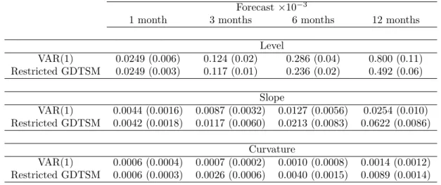
Recent empirical evidence suggests that excess returns to bonds are forecastable by a linear combination of forward rates (Cochrane and Piazzesi (2005)). Here, I construct a tractable arbitrage free dynamic term structure model (DTSM) with prices of risk that incorporate this predictability. Using a novel method to initialise the maximum likelihood procedure, the estimated model improves on the out-of-sample forecasting of the most important principle component of bond yields, the level component, compared to an unrestricted VAR(1). Given recent insight on the relationship between Gaussian DTSMs and the VAR(1) on principle components (Joslin, Singleton, and Zhu (2010)), the forecasting improvements provide some support for the restrictions on prices of risk imposed here.

(30)

2.1 Introduction

Bond yields are often studied using dynamic term structure models (DTSMs) - models that describe the co-movement over time of the entire yield curve. The Gaussian affine DTSM (GDTSM henceforth) is commonly applied in such studies. These are models in which the short rate,rt, is an affine function of a state vectorXt,rt=δ0,X+δT_XXt, and

Xtfollows a Gaussian affine diffusion under both the risk-adjusted (Q) and objective (P)

probability measures. Amongst several others, Duffee (2002), Ang and Piazzesi (2003) and Chernov and Mueller (2008) have explored the forecasting performance of GDTSMs. Recently, Joslin, Singleton, and Zhu (2010) (JSZ henceforth) have provided new insights into unrestricted GDTSMs (GDTSMs in which market prices of risk are left as free parameters). Loosely speaking, JSZ show that, regardless of the constraints imposed on the Q distribution of Xt, the forecasts implied by a GDTSM (estimated by

maxi-mum likelihood (ML)) and an unrestricted first order vector autoregression (VAR(1)) (estimated by ordinary least squares (OLS)) are identical. This means that, once given data on n accurately measured yields, then data on the shape of the remainder of the yield curve cannot in any way contribute to the model’s forecasting ability. Simply put, imposing no-arbitrage alone does not help in forecasting.

For researchers aiming to forecast future yields using a GDTSM, the above mentioned findings pose the important question, can the no-arbitrage restriction be used at all to improve yield forecasts? JSZ show formally that restrictions on market prices of risk (or, equivalently, on the P dynamics of Xt) are able to increase the efficiency of

yield forecasts compared with the VAR(1). The intuition behind their result can be understood as follows.

Consider, as an illustrative example, an economy in which interest rates are described by a GDTSM in which the local expectations hypothesis (LEH) holds. Under the LEH, tight restrictions are imposed on market prices of risk; they are zero. Investors are neutral to interest rate risk and so risk premia to long bonds and short bonds are both zero. An upward (downward) sloping yield curve must forecast rises (falls) in future short yields because that is the only way that high (low) yielding long bonds can have expected returns equal to those of a low (high) yielding short bonds over a given holding period. The key point to note is that, due to the restrictions on market prices of risk of the LEH, the arbitrage free cross section of yields has provided information about the time series of yields and hence we have the result mentioned above.

(31)

Although, in principle, imposing the LEH on a GDTSM allows the researcher to use no-arbitrage for forecasting, it has long been established that the restrictions on market prices of risk that are imposed by the LEH are empirically rejected (Fama and Bliss (1987), Campbell and Shiller (1991)). Such a GDTSM therefore provides poor yield forecasts. The actual forecasting efficiency of a GDTSM can only be increased if the restrictions on market prices of risk are consistent with the empirical facts relating to bond excess returns. The main purpose in this chapter is to construct such a model. I now introduce some of this empirical evidence.

The classic regressions of Fama and Bliss (1987) provide evidence that the one year excess return to the n-year bond can be forecast using the spread between the n-year forward rate and the one year yield with an R2 of 18%. Campbell and Shiller (1991) find related results when forecasting yield changes with yield spreads. More recently, Cochrane and Piazzesi (2005) (CP henceforth) were able to considerably improve on this predictability. They find that a single factor, a tent-shaped linear combination of forward rates, forecasts excess returns to bonds of one to five year maturity with an R2 of 44%.

The GDTSM in this chapter is motivated by the regressions of CP; risk premia to all bonds are determined by a linear combination of forward rates. The reason that it is possible to accommodate this predictability into a GDTSM can be understood as follows. It is easily shown that forward rates in a GDTSM are affine in the state vector. Further, a Gaussian essentially affine DTSM (first described by Duffee (2002)) allows market prices of risk to be affine in the state vector. Comparing the forward rate equation and the form of market prices of risk allows one to choose parameters such that market prices of risk (and hence risk premia) depend on forward rates. These ideas are made formal in Section 2.2 below.

Imposing the restrictions on market prices of risk just described is intended to improve the GDTSM’s forecasting. Given the results of JSZ, it is therefore natural to take the forecasts of a VAR(1) estimated by OLS as a benchmark for comparison. I find that the restrictions imposed here can improve out-of-sample forecasts.

The discussion so far has centered on how, via restrictions on market prices of risk in a GDTSM, the yield curve may improve yield forecasting. The other side of the same coin is that such restrictions can improve our understanding of the yield curve by making its decomposition into expectations and risk premium components more efficient.

(32)

Restrictions on market prices of risk link the time series (P dynamics) and cross section (Q dynamics) of bond yields and so the time series of bond yields helps estimate the Q parameters. Indeed, in estimating a GDTSM with restrictions on prices of risk by ML, the JSZ separation of the likelihood function into two parts that depend on only either the Q or P parameters is no longer generally possible; all parameters are estimated simultaneously.

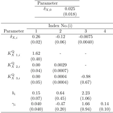
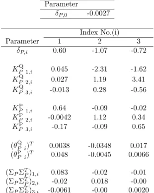
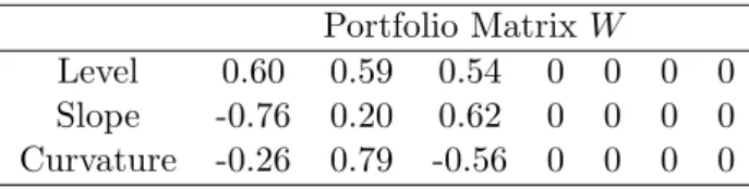
Given the above, another aim in this chapter is to understand risk premia in bond returns. The approach taken is to apply appropriate invariant transformations to the GDTSM’s parameters (as described in Dai and Singleton (2000)) so that each element in the state vector is a principle component of bond yields. The first three principle components (in order of decreasing variance/eigenvalues) are commonly labelled level, slope and curvature for the respective effects of shocks to them on the shape of the yield curve. The GDTSM is then estimated by ML. The approach of transforming to a GDTSM with principle components as the state vector has the following two main advantages.

One immediate advantage is in economic interpretation. It is both intuitive and now commonplace in the literature to decompose the variation in the yield curve into level, slope and curvature components; thinking of movements in the entire yield curve as being driven mainly by a small number of factors derives from the classic analyses of Knez, Litterman, and Scheinkman (1994) and Litterman and Scheinkman (1991). If, for example, risk to the level factor carries a high price, then this is perhaps more easily interpreted than risk to a latent factor (or even a particular yield) carrying a price. This is due to both the easy interpretation of the level factor, and the fact that this factor is orthogonal to other factors, meaning that the contributions to risk premia due to the different priced risks are neatly separated.

A second advantage of using the principle components (or, indeed, any n observable linearly independent combinations of bond yields) as the state vector is in econometric implementation. Despite the restrictions that are imposed on market prices of risk in the GDTSM estimated here, there are still a relatively large number of free parameters to optimise over in the ML procedure (17 in a 3 factor model). This can make it difficult to ensure that estimates resulting from the ML procedure are globally optimal.

One method by which researchers increase the chance that their ML procedure converges to the global optimum is to initialise the optimisation at many different locations and generate parameter estimates at each convergence. They then take as their ML estimates

(33)

those that correspond to the largest likelihood. This approach may be improved if there is some guidance as to suitable initialisation points. If the state vector is observable, then the parameters of an unrestricted VAR(1), quickly and consistently estimated by OLS, may provide a good initialisation point for some of the parameters in the model (means and mean reversion rates). Indeed, in the case of an unrestricted GDTSM, JSZ show that the OLS estimates are globally optimal. Subsection 2.4.6 devotes considerable attention to the initialisation problem. I show how one can choose suitable initialisation points for all the parameters in the model and simultaneously, via invariant transformations, maintain econometric identification.

More generally, imposing restrictions on market prices of risk carries the two econo-metric advantages that (i) there are fewer parameters to estimate and (ii) some of the parameters that are most difficult to estimate (those that affect drifts) have been re-moved. If the GDTSM is correctly specified then restrictions on prices of risk increase the efficiency of parameter estimates.

The remainder of this chapter proceeds as follows. I begin with a discussion of the related literature. I continue in Section 2.2 with a brief recapitulation of the bond pricing equation for affine GDTSMs provided by Duffie and Kan (1996) and I discuss the essentially affine form for market prices of Duffee (2002) that lie central to the GDTSM of this chapter. Section 2.3 specifies prices of risk such that risk premia to all bonds depend on a linear combination of forward rates. Next, Section 2.4 discusses the estimation problem, including transformations to an observable state vector and the ML procedure. Section 2.5 presents parameter estimates and measures of the GDTSM’s forecasting. Finally, Section 2.6 concludes.

2.1.1 Further Related Literature

The model presented in this chapter is most closely related to Cochrane and Piazzesi (2008), who also construct a GDTSM motivated by their earlier findings in CP. The main difference between their approach and that taken in this chapter is in implementation. These authors take the level, slope and curvature principle components as elements of the state vector, but also take a fourth factor: the linear combination of forward rates that drive market prices of risk. Their SDF allows only the level principle component to be priced and their model is chosen to exactly match the regressions in CP.

Duffee (2002) and Kim and Wright (2005) have estimated 3-factor unrestricted GDTSMs. Their models therefore nest the 3-factor GDTSM used here. One task in this chapter is

(34)

to compare the forecasting of the GDTSM with its unrestricted counterpart.

More generally, any DTSM consists of three components: (i) the dependence of the short rate of interest on the state vector, (ii) the dynamics of the state vector under the Q probability measure and (iii) a specification of market prices of risk (the SDF).

Points (i) and (ii) have been well studied (Subsection 1.1.1 discussed the relevant lit-erature). Focussing on (i) and (ii) is suitable for pricing derivatives on bonds where modelling bond volatility rather than expected return is of most importance. It is also useful for drawing smooth yield curves across maturities to either price bonds of non-traded maturities or, if the modeller believes strongly enough in the model, to arbitrage away any bonds that do not lie on the curve drawn. However, this approach is not suitable for bond portfolio analysis. For this, point (iii) must be addressed.

The more recent literature has focussed on point (iii). Duffee (2002), Dai and Singleton (2002) and Duarte (2004) are notable early contributions towards understanding bond prices in both the time series and cross section. The GDTSM presented in this chapter is also a contribution in this direction.

2.2 Affine Dynamic Term Structure Models

This section provides a brief recapitulation of the key results relating to the prices of bonds in the cross section and time series implied by GDTSMs. These results are sub-sequently used in Section 2.3 to construct the model central to this chapter: a GDTSM where risk premia to bonds depend on a linear combination of forward rates.

2.2.1 Affine Bond Pricing

Risk is generated in the economy by n Q-Brownian motions W_tQ ≡ (W_t,Q₁, . . . , W_t,nQ)T_.

The n-dimensional state vector is denotedXt≡(Xt,1, . . . , Xt,n)T and is driven byWtQ.

The short rate of interest,rt, is an affine function of the state vector:

rt=δ0,X+δXTXt. (2.1)

Here δ0,X is a scalar andδX is ann-vector.

Throughout this chapter, the X subscript to parameters denotes that they enter the model in the form given in (2.1) (and below in (2.2) and (2.21)) when the state vector is Xt. This notation is useful later when I make invariant transformations to different state

(35)

vectors. For example, ifYtis used as the state vector then I write rt=δ0,Y +δTYYt and,

of course,δ0,Y and δY are related to δ0,X and δX in a way that depends on the relation

between Yt and Xt. I return to this topic in Subsection 2.3.4. A similar approach to

notation is taken with functions and matrices that depend on parameters. GDTSMs impose that the Q evolution of the state vector is described by

dXt=K_XQ

θ_XQ−Xt

dt+ ΣXdWtQ, (2.2)

whereK_XQ and ΣX aren×n matrices andθQX is ann-vector.

Duffie and Kan (1996) show that, in this framework, the time t price of the time T maturity zero-coupon bond is given by

Pt(u) =PX(Xt, u)≡eAX(u)−BX(u) T_X

t_. _(2.3)

Here,u≡T−t,AX(u) is a scalar function andBX(u) is ann-valued function. These are

the solutions to the system of Riccati ordinary differential equations (ODEs), provided in Subsection 2.7.1 in the appendix to this chapter. Given (2.3), the bond yield defined by yt(u)≡ − 1 ulnPt(u) (2.4) is given by yt(u) = 1 u(−AX(u) +BX(u) T_X t). (2.5)

Finally, letting ft(u) denote the time tinstantaneous forward rate that prevails at time

t+u, it is a standard no-arbitrage result that

ft(u) =− ∂ ∂ulogPX(Xt, u) =− ∂AX(u) ∂u + ∂BX(u)T ∂u Xt. (2.6)

(2.3) provides the time t conditional prices of the cross section of bond maturities. However, we are yet to make a statement about conditional expected returns to bonds in the time series. For this we must specify the market prices of risk.

(36)

2.2.2 Expected Returns to Bonds The SDF, denoted by πt, follows the process

dπt

πt

=−rtdt−ΛTtdWtP,

whereW_tP ≡(W_t,P₁, . . . , W_t,nP)T is ann-vector of P-Brownian motions and Λtis a column

n-vector specifying market prices of risk. Applying Girsanov’s theorem to (2.2) gives the dynamics of the state vector under the P measure as

dXt=K_XQ

θQ_X −Xt

dt+ ΣXΛtdt+ ΣXdWtP. (2.7)

The bond pricing function solves dPX(Xt, u)

PX(Xt, u)

= (rt+et(u))dt+vt(u)TdWtP, (2.8)

whereet(u) is a scalar that denotes the time tinstantaneous risk premium to holding a

bond that matures at time t+u. vt(u) is an n-vector that determines the volatility of

this bond. An application of It¯o’s lemma to (2.3) and using (2.7) reveals that these two quantities are given by

et(u) ≡ −BX(u)TΣXΛt and (2.9)

vt(u)T ≡ −BX(u)TΣX.

The GDTSM is not yet fully specified; (2.9) shows that we must choose a Λtto determine

risk premia. The choice of form for Λtis delicate. It must be sufficiently flexible to ensure

that the model is able to capture the key feature of the data that we wish to expose (that expected excess returns to bonds are linear in forward rates) but also restricted enough so that the model remains econometrically tractable. An essentially affine specification, given in the next subsection, is suitable for this task.

2.2.3 Essentially Affine Market Prices of Risk

When the state vector follows a Gaussian affine process, the essentially affine specifica-tion for the market price of risk vector is

Λt≡λ0,X +λ1,XXt, (2.10)

whereλ0,X andλ1,X are anndimensional column vector andn×nmatrix of parameters

(37)

depend on the parameters that governXt. This will become clear below.

The equations for the short rate, the Q-dynamics and the market prices of risk in terms of the state vector, given in (2.1), (2.2) and (2.10) respectively, completely specify the GDTSM in the sense that the statistical properties of bond prices in both the time series and in the cross section of bond maturities are pinned down. The aim is to make risk premia depend on a linear combination of forward rates. By inspecting (2.10) and the equation for forward rates in (2.6) it is immediately apparent that, with appropriate choices of λ0,X andλ1,X, it is possible to ensure this aim. The next step is to formalise

this observation.

2.3 Model Specification

CP provide motivation for choosing Λt such that risk premia to all bonds depend on a

linear combination of forward rates. The main purpose in this section is to choose such a Λt.

2.3.1 Prices of Risk

Recall that there arenstate variables. Define the following n-vector

et≡(et(u1), . . . , et(un))T. (2.11)

Here, et denotes the risk premia to n bonds with times to maturity of u1, . . ., un

respectively. The meaning ofet(ui) can be understood from (2.8).

In the model, risk premia to the set ofnbonds that enteret(those with times to maturity

of u1, . . . , un) and also all other bonds will depend on a linear combination of forward

rates. However, the nbonds that enteret are special in the sense that their risk premia

can be specified independently of one another and explicitly in terms of free parameters that enter the GDTSM. Given the risk premia to the bonds inet, risk premia to all other

bonds are then determined by the no-arbitrage relationship in (2.9). This idea is made formal below, but the intuition as to why the risk premia to exactly n bonds can be specified explicitly and independently of one another in a model with n state variables can be understood as follows.

Without loss of generality, one can let the n state variables in the GDTSM be n or-thogonal observable combinations of yields (principle components); based on Dai and Singleton (2000), Subsection 2.4.3 makes transformations that allow one to change from

(38)

latent to observable combinations of yields as state variables whilst leaving the short rate and hence bond prices unchanged. Since the principle components are othogonal to one another, there is no reason that the risk premium associated with shocks to each of them must be related to each other. In other words, we must be able to specify the risk premia to thesencombinations of bonds separately of one another.

The next step is to write et in terms of forward rates. Let ft denote an (m+ 1)-vector

that consists of a constant and themforward rates that will drive risk premia. Recalling from (2.6) thatft(v) denotes the timetinstantaneous forward rate that prevails at time

t+v, I define

ft≡[1ft(v1) . . . ft(vm)]T.

Note thatm is allowed to be different from n. Making risk premia to then bonds that enter et linear in forward rates requires that

et=bγTft. (2.12)

Here b and γ are n×1 and (m+ 1)×1 vectors of parameters respectively. Clearly, for the purposes of model estimation, the b and γ are not separately identified and so appropriate normalisations are imposed (see Section 2.4). The scalar, γTft, drives risk

premia and the i-th entry in the vectorb, bi, gives the loadings of the risk premium of

the ui maturity bond on this factor. Therefore, as discussed above, the risk premia to

then bonds inet can be determined separately to each other. However, risk premia to

bonds of all maturities and not just theu1, . . . , unmaturity bonds have been determined

via (2.9); a fully specified DTSM describes the co-movement over time of the entire yield curve.

The parameters b and γ do not have X subscripts because these parameter do not change under invariant transformations of the GDTSM’s state vector. The reason is clear; expected returns to bonds should be the same in all observationally equivalent models, regardless of the choice of state vector.

Simple algebraic manipulation of (2.9), (2.11) and (2.12) then gives the market price of risk vector as

Λt=−Σ−_X1B_X−1bγTft, (2.13)

where

(39)

Equation (2.13) assumes that BX is invertible. The invertibility of BX is guaranteed

by assuming that no two bonds yields in the set of bonds with maturites u1, . . . , un are

proportional to each other. This is clear from (2.5); if no two yields are proportional to each other then the rows of BX must be linearly independent.

2.3.2 Forward Rates in Terms of the State Vector

The elements of vectorft are all affine in the state variables. This can be seen from the

standard no-arbitrage result that

ft(u) =−

∂

∂ulogPt(u) (2.15)

and an application of (1.2) to give

ft(u) =−

∂AX(u)

∂u +

∂BX(u)T

∂u Xt. (2.16)

We can then define an (m+ 1)×1 vector F0,X and an (m+ 1)×n matrix F1,X such

that

ft=F0,X+F1,XXt. (2.17)

In the above equation,

F0,X ≡ − −1 ∂AX(s) ∂s s=v1 . . . ∂AX(s) ∂s s=vm T , (2.18) and F1,X ≡         0T_n ∂BX(s)T ∂u s=v1 .. . ∂BX(s)T ∂u s=vm         . (2.19)

Here, 0nis an n-vector of zeros.

Given (2.17), the price of risk vector in (2.13) can then be written in the essentially affine form given in (2.10). The quantities λ0,X and λ1,X are

λ0,X = −Σ−_X1B_X−1bγTF0,X, (2.20)

λ1,X = −Σ−_X1B_X−1bγTF1,X.