Edinburgh Research Explorer

Edinburgh Research Explorer

Canonical Correlation Inference for Mapping Abstract Scenes to

Text

Citation for published version:

Papasarantopoulos, N, Jiang, H & Cohen, S 2018, Canonical Correlation Inference for Mapping Abstract Scenes to Text. in Proceedings of the Thirty-Second AAAI Conference on Artificial Intelligence (AAAI-18). Association for the Advancement of Artificial Intelligence, pp. 5358-5365, Thirty-Second AAAI Conference on Artificial Intelligence, New Orleans, United States, 2/02/18.

<https://www.aaai.org/ocs/index.php/AAAI/AAAI18/paper/view/16365/16088>

Link:

Link to publication record in Edinburgh Research Explorer Document Version:

Peer reviewed version

Published In:

Proceedings of the Thirty-Second AAAI Conference on Artificial Intelligence (AAAI-18)

General rights

Copyright for the publications made accessible via the Edinburgh Research Explorer is retained by the author(s) and / or other copyright owners and it is a condition of accessing these publications that users recognise and abide by the legal requirements associated with these rights.

Take down policy

The University of Edinburgh has made every reasonable effort to ensure that Edinburgh Research Explorer content complies with UK legislation. If you believe that the public display of this file breaches copyright please contact [email protected] providing details, and we will remove access to the work immediately and investigate your claim.

Canonical Correlation Inference for Mapping Abstract Scenes to Text

Nikos Papasarantopoulos

Helen Jiang

Department of Computer Science Stanford University [email protected]

Shay B. Cohen

We describe a technique for structured prediction, based on canonical correlation analysis. Our learning algorithm finds two projections for the input and the output spaces that aim at projecting a given input and its correct output into points close to each other. We demonstrate our technique on a language-vision problem, namely the problem of giving a tex-tual description to an “abstract scene.”

1

Introduction

Canonical correlation analysis (CCA) is a method to re-duce the dimensionality of multiview data, introre-duced by Hotelling (1935). It takes two random vectors and com-putes their corresponding empirical cross-covariance matrix. It then applies singular value decomposition (SVD) on this matrix to get linear projections of the random vectors that have maximal correlation.

In this paper, we investigate the idea of using CCA for a full-fledged structured prediction problem. More specif-ically, we suggest a method in which we take a structured prediction problem training set, and then project both the in-puts and the outin-puts to low-dimensional space. The projec-tion ensures that inputs and outputs that correspond to each other are projected to close points in low-dimensional space. Decoding happens in the low-dimensional space. As such, our training algorithm builds on previous work by Udupa and Khapra (2010) and Jagarlamudi and Daum´e III (2012) who used CCA for transliteration.

Our approach of canonical correlation inference is simple to implement and does not require complex engineering tai-lored to the task. It mainly needs two feature functions, one for the input values and one for the output values and does not require features combining the two. We also propose a simple decoding algorithm when the output space is text.

We test our learning algorithm on the domain of language and vision. We use theabstract scenedataset of Zitnick and Parikh (2013), with the goal of mapping images (in the form of clipart abstract scenes) to their corresponding image de-scriptions. This problem has a strong relationship to recent work in language and vision that has used neural networks Copyright c2018, Association for the Advancement of Artificial Intelligence (www.aaai.org). All rights reserved.

or other computer vision techniques to solve a similar prob-lem for real images (Section 2.2). Our work is most closely related to the work by Ortiz, Wolff, and Lapata (2015) who used phrase-based machine translation to translate images to corresponding descriptions.

2

Background and Notation

We give in this section some background information about CCA and the problem which we aim to solve with it.

2.1

Canonical Correlation Analysis

Canonical correlation analysis (CCA; Hotelling, 1935) is a technique for multiview dimensionality reduction, related to co-training (Blum and Mitchell 1998). CCA assumes that there are two views for a given set of data, where these two views are represented by two random vectorsX ∈Rdand

Y ∈_Rd0_.

The procedure that CCA follows finds a projection of the two views in a shared space of dimension m, such that the correlation between the two views is maximized at each coordinate, and there is minimal redundancy be-tween the coordinates of each view. This means that CCA solves the following sequence of optimization problems for

j∈ {1, . . . , m}whereaj ∈R1×dandbj ∈R1×d 0 : arg max aj,bj corr(ajX>, bjY>)

such that corr(ajX>, akX>) = 0, k < j corr(bjY>, bkY>) = 0, k < j

wherecorris a function that accepts two vectors and returns the Pearson correlation between the pairwise elements of the two vectors. The problem of CCA can be solved by applying singular value decomposition (SVD) on a cross-covariance matrix between the two random vectorsX andY, normal-ized by the covariance matrices ofXandY.

More specifically, CCA is solved by applying thin singu-lar value decomposition (SVD) on the empirical version of the following matrix:

(E[XX>])−12E[XY>](E[Y Y>])− 1

2 ≈UΣV>,

whereE[·]is the expectation operator andΣis a diagonal matrix of sizem×mfor some smallm. Since this version

of CCA requires inverting matrices of potentially large di-mension (d×dandd0×d0), it is often the case that only the diagonal elements from these matrices are used, as we see in Section 3.

CCA and its variants have been used in various con-texts in NLP. They were used to derive word embeddings (Dhillon, Foster, and Ungar 2015), derive multilingual em-beddings (Faruqui and Dyer 2014; Lu et al. 2015), build bilingual lexicons (Haghighi et al. 2008), encode prior knowledge into embeddings (Osborne, Narayan, and Co-hen 2016), semantically analyze text (Vinokourov, Cristian-ini, and Shawe-Taylor 2002) and reduce the dimensions of text with many views (Rastogi, Van Durme, and Arora 2015). CCA is also an important sub-routine in the family of spectral algorithms for estimating structured models such as latent-variable PCFGs and HMMs (Cohen et al. 2012; Stratos, Collins, and Hsu 2016) or finding word clusters (Stratos et al. 2014). Variants of it have been developed, such as DeepCCA (Andrew et al. 2013).

2.2

Describing Images

Image description, the task of assigning textual descriptions to images, is a problem that has been thoroughly studied in various setups and variances. Usually, proposed methods treat images as sets of objects identified in them (bags of regions), however there has been work that uses some kind of structural image cues or relations. An excellent example of such cues are visual dependency representations (Elliott and Keller 2013), which can be used to outline what can be described as the visual counterpart of dependency trees.

Common is also the idea of solving a related but slightly different problem, the one of matching sentences to images using existing descriptions. The core of those approaches is an information retrieval task, where for every novel image, a set of similar images is retrieved and generation proceeds using the descriptions of those images. Search queries are posed against a visual space (Ordonez, Kulkarni, and Berg 2011; Mason and Charniak 2014) or a multimodal space, where images and descriptions have been projected (Farhadi et al. 2010; Hodosh, Young, and Hockenmaier 2013). In-stead of whole sentences, phrases from existing human gen-erated descriptions have also been used (Kuznetsova et al. 2012).

Approaches to image description generation have for a long time relied on a set of predefined sentence templates (Kulkarni et al. 2011; Elliott and Keller 2013; Yang et al. 2011) or used syntactic trees (Mitchell et al. 2012), while more recently, methods that use neural models (Kiros, Salakhutdinov, and Zemel 2014; Vinyals et al. 2015) have appeared, that avoid the use of any kind of predefined pat-tern. Approaches like the latter follow the paradigm of tack-ling the problem as an end-to-end optimization problem. Or-tiz, Wolff, and Lapata (2015) describe a two-step process: a content selection phase, where the objects that need to be de-scribed are picked, and then the text realization, where the description is generated by employing a statistical machine translation (MT) system.

While computer vision advances have given an unprece-dented potential to image description generation, vision

per-formance affects the generation process, as those two prob-lems are commonly solved together in a pipeline or a joint fashion. To countermeasure that, Zitnick and Parikh (2013) introduced the notion of “abstract scenes”, that is abstract images generated by stitching together clipart images. Their intuition is that working on abstract scenes can allow for a more clean and isolated evaluation of caption generators and also lead to relatively easy construction of datasets of images with semantically similar content. An example of such dataset is the Abstract Scenes Dataset.1 This dataset has been used for description generation (Ortiz, Wolff, and Lapata 2015), sentence-to-scene generation (Zitnick, Parikh, and Vanderwende 2013) and object dynamics prediction (Fouhey and Zitnick 2014) so far.

3

Learning and Decoding

We now describe the learning algorithm, based on CCA, and the corresponding decoding algorithm when the output space is text.

3.1

Learning Based on Canonical Correlation

Analysis

We assume two structured spaces, an input spaceX and an output spaceY. As usual in the supervised setting, we are given a set of instances(x1, y1), . . . ,(xn, yn)∈ X × Y, and

the goal is to learn a decoderdec :X → Ysuch thatdec(x)

is the “correct” output as learned based on the training ex-amples.

The basic idea in our learning procedure is to learn two projection functionsu:X →Rmandv:Y →Rmfor some low-dimensionalm(relatively todandd0). In addition, we assume the existence of a similarity measureρ:Rm×Rm→ Rsuch that for anyxandy, the bettery “matches” thex according to the training data, the larger ρ(u(x), v(y))is. The decoderdec(x)is then defined as:

dec(x) = arg max

y∈Y ρ(u(x), v(y)). (1)

Our key observation is that one can use canonical cor-relation analysis to learn the two projections u and v. This is similar to the observation made by Udupa and Khapra (2010) and Jagarlamudi and Daum´e III (2012) in previous work about transliteration. The learning algorithm assumes the existence of two feature functions φ: X →

Rd×1andψ:Y →Rd 0_×1

, wheredandd0could potentially be large, and the feature functions could potentially lead to sparse vectors.

We then apply a modified version of canonical correla-tion analysis on the two “views:” one view corresponds to the input feature function and the other view corresponds to the output feature function. This means we calculate the following three matrices D1 ∈ Rd×d, D2 ∈ Rd

0_×d0 and Ω∈Rd×d 0 : 1 https://vision.ece.vt.edu/clipart/

Inputs: Set of examples (xi, yi) ∈ X × Y for i ∈

{1, . . . , n}. An integerm. Two feature functionsφ(x)and

ψ(y).

Data structures:

Projection matricesUandV. Algorithm: (Cross-covariance estimation) • CalculateΩ∈Rd×d 0 Ωij= n X k=1 [φ(xk)]i[ψ(yk)]j

• CalculateD1 ∈ Rd×dsuch that(D1)ij = 0fori 6= j

and (D1)ii= n X k=1 [φ(xk)]i[φ(xk)]i • CalculateD2 ∈Rd 0_×d0

such that(D2)ij = 0fori6=j

and (D2)ii= n X k=1 [ψ(yk)]i[ψ(yk)]i

(Singular value decomposition step) Calculatem-rank thin SVD on D−

1 2 1 ΩD −1 2 2 . Let U and

V be the two resulting projection matrices. Return the two functions u(x) = (D− 1 2 1 U) > φ(x) and v(y) = (D−12 2 V) > ψ(y).

Figure 1: The CCA learning algorithm.

D1= diag 1 n n X i=1 φ(xi)(φ(xi))> ! D2= diag 1 n n X i=1 ψ(yi)(ψ(yi))> ! Ω = 1 n n X i=1 φ(xi)(ψ(yi))>

wherediag(A)for a square matrixA is a diagonal matrix with the diagonal copied fromA. We then apply thin singu-lar value decomposition onD−1₁ /2ΩD−1₂ /2so that

D₁−1/2ΩD₂−1/2≈UΣV>,

withU ∈ _Rd×m_{,Σ ∈}

Rm×mis a diagonal matrix of sin-gular values andV ∈ Rd

0_×m

. The value ofm should be relatively small compared tod andd0_{. We then chooseu}

andvto be: u(x) = (D−12 1 U)>φ(x), v(y) = (D− 1 2 2 V) >_ψ(y).

For the similarity metric, we use the cosine similarity:

ρ(z, z0) = Pm i=1zizi0 pPm i=1z 2 i pPm i=1(z 0 i)2 = hz, z 0_i ||z|| · ||z0_||.

Figure 2 describes a sketch of our CCA inference algo-rithm.

Motivation What is the motivation behind this use of

CCA and the chosen projection matrices and similarity met-ric? Osborne, Narayan, and Cohen (2016) showed that CCA maximizes the following objective:

X i,j dij−n n X i=1 d2_ii, where dij= v u u t 1 2 m X k=1 (u(xi)−v(yj))2 ! .

The objective is maximized with respect to the projections that CCA finds,uandv. This means that CCA finds pro-jections such that the Euclidean distance betweenu(x)and

v(y)for matchingxandy is minimized, while it is maxi-mized forxandythat have a mismatch between them.

As such, it is well-motivated to use a similarity metric

ρ(u(x), v(y))which is inversely monotone with respect to the Euclidean distance betweenu(x)andv(y). We next note that for any two vectorsz(denotingu(x)) andz0 _(denoting

v(y)) it holds that (by simple algebraic manipulation):

−hz, z0i= 1

2 ||z−z 0_||2

− ||z||2− ||z0||2

. (2)

This means that if the norms of z andz0 are constant, then maximizing the cosine similarity between zandz0 is the same as minimizing Euclidean distance betweenzand

z0. In our case, the norms ofu(x)andv(y)are not constant, but we find that our algorithm is much more stable when the cosine similarity is used instead of the Euclidean distance.

We also note that in order to minimize the distance be-tweenzandz0_{to follow CCA, according to Eq. 2, we need}

tomaximizethe dot product betweenz andz0 while mini-mizing the norm ofzandz0. This is indeed the recipe that the cosine similarity metric follows.

In Section 3.2 we give an additional interpretation to the use of cosine similarity, as finding the maximum aposteriori solution for a re-normalized von Mises-Fisher distribution.

3.2

When the Output Space is Language

While our approach to mapping from an input space to an output space through CCA is rather abstract and general, in this paper we focus in cases where the output spaceY ⊆Λ∗

θ

Jenny is holding an owl.

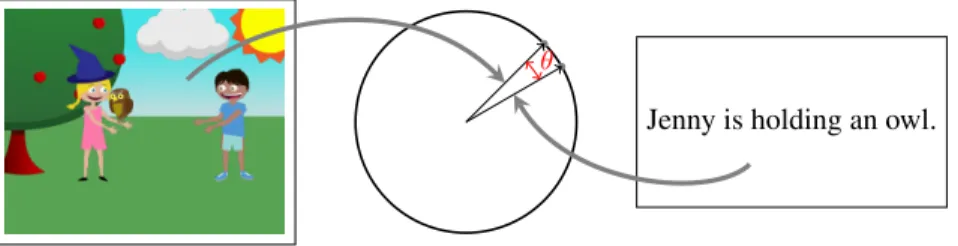
Figure 2: Demonstration of CCA inference. An object from the input spaceX (the image on the leftx) is mapped to a unit vector. Then, we find the closest unit vector which has an embodiment in the output space,Y. That embodiment is the text on the right,y. It also also holds thatρ(u(x), v(y)) = cosθ.

English language. For example,Ycould be the set of alln -gram chains possible over somen-gram set or the set of pos-sible composition of atomic phrases, similar to phrase tables in phrase-based machine translation (Koehn et al. 2007).

For the language-vision problem we address in Section 4, we assume the existence of a phrase tableP, such that every

y ∈ Y can be decomposed into a sequence of consecutive phrasesp1, . . . , pr∈ P.

The problem of decoding over this space is not trivial. This is regardless ofX– oncexis given, it is mapped using

u(x)to a vector inRm, and at this point this is the infor-mation we use to further decode intoy– the structure ofX

before this transformation does not change much the com-plexity of the problem. We propose the following approx-imate decoding algorithmdec(x)for Eq. 1. The algorithm is a Metropolis-Hastings (MH) algorithm that assumes the existence of a blackbox sampler q(y | y0)– the proposal distribution. This blackbox sampler randomly chooses two endpointskand`iny0and if possible, replaces all the words in between these two words (y<sub>k</sub>0 · · ·y<sub>`</sub>0) with a phrasep∈ P

such that in the training data, there is an occurrence of the new phrasepafter the wordy_k0₋₁and before the wordy_`0₊₁. As such, we are required to create a probabilistic table of the formQ: Λ× P ×Λ → Rthat maps a pair of words

y, y0 ∈Λand a phrasep∈ Pto the probabilityQ(p|y, y0). In our experiments, we use the phrase table used by Ortiz, Wolff, and Lapata (2015), extracted using Moses, and use relative frequency count to estimateQ: we count the number of times each phrasepappears between the context wordsy

andy0and normalize.

Since we are interested inmaximizingthe cosine similar-ity between v(y) and u(x), after each sampling step, we check whether the cosine similarity of the newy is higher (regardless of whether it is being accepted or rejected by the MH algorithm) than that of anyyso far. We return the best

ysampled.

The “true” unnormalized distribution we use in the accept-rejection step is the exponentiated value of the co-sine similarity betweenu(x)andv(y). This means that for a given x, the MH algorithm implicitly samples from the following distributionP:

Inputs:An input examplex, a similarity metricρ, two pro-jection functionsuandv, a probabilistic phrase tableQ, a constantη≥0, a constantτ ∈(0,1), a starting temperature

T.

Algorithm: (Initialization)

• Lety∗be an arbitrary point in the output space. • Lety0bey∗.

• LettbeT.

While the temperaturetgoes below a given value:

• Choose uniformly two different integers between1and |y0|, the length ofy0,iandj.

• Choose randomly a phrasepfromQ(p|yi0−1, y

0 j+1). • Lety=y10· · ·y 0 i−1py 0 j+1· · ·y 0 |y0|. • Ifρ(u(x), v(y)) +η|y| ≥ ρ(u(x), v(y∗)) +η|y0|, then sety∗to bey. • Let α0= exp 1 tρ(u(x), v(y)) +η|y| exp 1 tρ(u(x), v(y 0 )) +η|y0| α1= |y|2 Q(yi0· · ·y 0 j|y 0 i−1, y 0 j+1) |y0_|2_Q(y i· · ·yj|yi−1, yj+1) α={1, α0·α1}.

• Uniformly sample a number from[0,1], and if it is smaller thanα, sety0to bey.

• Lett←τ t. Returny∗.

Figure 3: The CCA decoding algorithm.

P(y|x) = exp _{hu(x), v(y)i} ||u(x)|| · ||v(y)|| Z(x) (3) where

Z(x) = X y0_∈Y exp hu(x), v(y0)i ||u(x)|| · ||v(y0_)|| .

The probability distributionP has a strong relationship to the von Mises-Fisher distribution, which is defined over vectors of unit vector. The von Mises-Fisher distribution has a parametric density functionf(z;µ)which is proportional to the exponentiated dot product between the unit vectorz

and some other unit vector µ which serves as the param-eter for the distribution. The main difference between the von Mises-Fisher distribution and the distribution defined in Eq. 3 is that we do not allowanyunit vector to be used as

v(y)

||v(y)|| – only those which originate in some output

struc-turey. As such, the distribution in Eq. 3 is a re-normalized version of the von-Mises distribution, after elements from its support are removed.

In a set of preliminary experiments, we found that while our algorithm gives adequate descriptions to the images, it is not unusual for it to give short descriptions that just mention a single object in the image. This relates to the adequacy-fluency tension that exists in machine translation problems. To overcome this issue, we add to the cosine similarity a termη|y|whereηis some positive constant tuned on a de-velopment set and|y|is the length of the sampled sentence. This pushes the decoding algorithm to prefer textual descrip-tions which are longer.

Simulated Annealing Since we are not interested in

sam-plingfrom the distribution P(y | x), but actually find its mode, we use simulated annealing with our MH sampler. This means that we exponentiate by a 1

t term the

unnormal-ized distribution we sample from, and decrease this temper-aturetas the sampler advances. We start with a temperature

T = 10,000, and multiplytbyτ = 0.995at each step. The idea is for the sampler to start with an exploratory phase, where it is jumping from different parts of the search space to others. As the temperature decreases, the sampler makes smaller jumps with the hope that it has gotten closer to parts of the search space where most of the probability mass is concentrated.

4

Experiments

Our experiments are performed on a language-vision dataset, with the goal of taking a so-called “abstract scene” (Zitnick and Parikh 2013) and finding a suitable textual de-scription. Figure 2 gives a description of our CCA algorithm in the context of this problem.

The Abstract Scenes Dataset consists of 10,020 scenes, each represented as a set of clipart objects placed in different positions and sizes in a background image (consisting of a grassy area and sky). Cliparts can appear in different ways, for example, the boy and the girl (cliparts 18 and 19), can be depicted sad, angry, sitting or running. The descriptions were given using crowdsourcing.

We use the same data split as Ortiz, Wolff, and Lap-ata (2015). We use 7,014 of the scenes as a training set,

y p y0 prob.

waiting to get 1.000

with the bucket. 0.750

pizza on the 0.343

trying to get away from jenny 0.050

baseball with the 0.033

is playing near the swings. 0.011 hbegini jenny is playing with a colorful 0.008 is surprised by the owl 0.006 mike and the bear are standing 0.002

Table 1: Example of phrases and their probabilities learned for the functionQ(p|y, y0). The markerhbeginimarks the beginning of a sentence.

1,002 as a development set and 2,004 as a test set.2 _Each scene is labeled with at most eight short captions. We use all of these captions in the training set, leading to a total of 42,276 training instances. We also use these captions as ref-erence captions for both the development and the test set.

The feature function φ(x)for an image is based on the “visual features” that come with the abstract scene dataset. More specifically, there are binary features that fire for 11 object categories, 58 specific objects, co-occurrence of ob-ject category pairs, co-occurrence of obob-ject instance pairs, absolute location of object categories and instances, absolute depth, relative location of objects, relative location with di-rectionality the object is facing, a feature indicating whether an object is near a child’s hand or a child’s head and at-tributes of the children (pose and facial expression). The total number of features for this φfunction is 7,149. See more in the description of the abstract scene dataset.

The feature functionψ(y)for an image description is de-fined as a one-hot representation for all phrases from the phrase table of Ortiz, Wolff, and Lapata (2015) that fire in the image (the phrase table is denoted by P in Sec-tion 3.2). This phrase table was obtained through the Moses toolkit (Koehn et al. 2007). The total number of phrases in this phrase table is 30,911. The size of the domain of Q

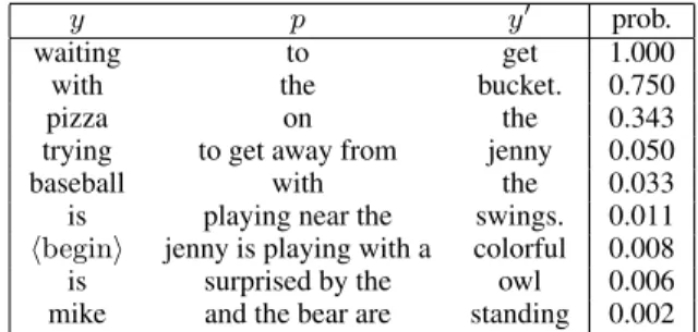
(meaning, the size of the phrase table with context words) is 120,019. Table 1 gives a few example phrases and their corresponding probabilities.

In our CCA learning algorithm, we also need to decide on the value ofm. We variedmbetween30and300(in steps of

10) and tuned its value on the development set by maximiz-ing BLEU score against the set of references.3_{Interestingly} enough, the BLEU scores did not change that much (they usually were within one point of each other for sufficiently largem), pointing to a stability of the algorithm with respect to the number of dimensions used.

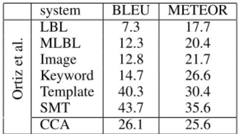
Ortiz, Wolff, and Lapata (2015) partially measure the suc-cess of their system by comparing BLEU and METEOR scores of their different systems while using the descriptions given in the dataset as a reference set. The scores for their

2

Our dataset splits and other information can be found in http://cohort.inf.ed.ac.uk/ canonical-correlation-inference.html.

3

We use themultevalpackage fromhttps://github. com/jhclark/multeval.

Figure 4: Scatter plot of SMT (statistical machine transla-tion) and CCA BLEU scores versus human ratings.

different systems are given in Table 2. They compare their system (SMT, based on phrase-based machine translation) against several baselines:4

• LBL: a log-bilinear language model trained on the image captions only.

• MLBL: mutlimodal log-bilinear model, implementation of Kiros, Salakhutdinov, and Zemel (2014).

• Image: a system that for every new image, queries the set

of training images for the most similar one, and returns a random description of that training example.

• Keyword: system that annotates every image with

key-words that most probably describe it and then do a search query against all training data descriptions, returning the description that is closest (in terms of TF-IDF similarity) to the keywords.

• Template: system that uses templates inferred from

de-pendency parses of the training data descriptions. A set of templates is discovered and a classifier that associates images with templates is trained.

• SMT: Ortiz et al. system first selects pairs of clipart ob-jects that are important enough to be described by solving an integer linear programming problem, creates a “visual encoding” using visual dependency grammar and finally uses a phrase-based SMT engine to translate the latter to proper sentences.

Our system does not score as high as their machine trans-lation system.

It is important to note that the descriptions given in the dataset, as well as those generated by the different systems are not “complete.” Each one of them describes a specific

4

We note that we also experimented with a neural network model (SEQ2SEQmodel), but it performed badly, giving a BLEU score of 10.20 and a METEOR score of 15.20 with inappropriate captions. It seems like SEQ2SEQmodels is unfit for this dataset, perhaps because of its size. See also Rastogi, Cotterell, and Eis-ner (2016) for similar results.

system BLEU METEOR

Ortiz et al. LBL 7.3 17.7 MLBL 12.3 20.4 Image 12.8 21.7 Keyword 14.7 26.6 Template 40.3 30.4 SMT 43.7 35.6 CCA 26.1 25.6

Table 2: Scene description evaluation results on the test set, comparing the systems from Ortiz et al. to our CCA in-ference algorithm (the first six results are reported from the Ortiz et al. paper). The CCA result uses m = 120and

η = 0.05, tuned on the development set. See text for details about each of the first six baselines.

Figure 5: An image with the following descriptions in the dataset: (1)mike is kicking the soccer ball; (2) mike is sitting on the cat; (3) jenny is standing next to the dog; (4) jenny is kicking the soccer ball; (5) the sun is behind jenny; (6) the soccer ball is under the sun.

bit of information that is implied by the scene. Figure 5 demonstrates this. As such, the calculation of SMT evalua-tion scores with respect to a reference set is not necessarily the best mechanism to identify the correctness of a textual description. To demonstrate this point, we measure BLEU scores of one of the reference sentences while comparing it to the other references in the set. We did that for each of the eight batches of references available in the training set.

The average reference BLEU score is 24.1 and the av-erage METEOR score is 20.0, a significant drop compared to the machine translation system of Ortiz, Wolff, and La-pata (2015). We concluded from this result that the SMT system is not “creatively” mapping the images to their cor-responding descriptions. It relies heavily on the training set captions, and learns how to map images to sentences in a manner which does not generalize very well outside of the training set.

Another indication that our system creates a more diverse set of captions is that the number ofuniquecaptions it gen-erates for the test set is significantly larger than that of the SMT system by Ortiz et al. The SMT system generates 359 unique captions (out of 2,004 instances in the test set), while CCA generates 496 captions, an increase of 38.1%.

To test this hypothesis about caption diversity, we con-ducted the following human experiment. We asked 12 sub-jects to rate the captions of 300 abstract scenes with a score

SMT jenny is waving at mike jenny is wearing a baseball jenny is holding a frisbee CCA mike and jenny are camping mike is holding a bat jenny is throwing the frisbee

SMT jenny is kicking the soccer ball jenny is holding a hot dog jenny is holding a hamburger CCA mike is kicking a blass jenny wants the bear the rocket is behind mike

Figure 6: Examples of outputs from the machine translation system and from CCA inference. The top three images give examples where the CCA inference outputs were rated highly by human evaluations (4 or 5), and the SMT ones were rated poorly (1 or 2). The bottom three pictures give the reverse case.

slice CCA<3 CCA≥3

SMT<3 M:1.77 M:1.92 C:1.64 C:3.71 SMT≥3 M:3.42 M:3.46 C:1.47 C:3.54

Table 3: Average ranking by human judges for cases in which the caption has an average rank of3 or higher (for both CCA and SMT) and when its average rank is lower than3. “M” stands for SMT average rank and “C” stands for CCA average rank.

between 1 to 5.5 Each rater was presented with three cap-tions: a reference caption (selected randomly from the gold-standard captions), an SMT caption and a caption from our system (presented in a random order) and was asked to rate the captions on adequacy level (on a scale of 1 to 5). Most images were rated exactly twice, with a few images getting three raters. A score of 1 or 2 means that the caption likely does not adequately describe the scene. A score of 3 usually means that the caption describes some salient component in the scene, but perhaps not the most important one. Scores of 4 and 5 usually denote good captions that adequately de-scribe the corresponding scenes. This experiment is similar to the one done by Ortiz et al.

The ranking results are given in Table 3. The results show that our system tends to score higher for images which are highly ranked (by both the SMT system and CCA), but tends to score lower for images which are lower ranked.

In addition, we checked the MT evaluation scores for highly ranked captions both for SMT and CCA (ranking larger than 4). For SMT, the BLEU scores are 49.70

(ME-5

The ratings can be found here:http://cohort.inf.ed. ac.uk/canonical-correlation-inference.html.

TEOR 40.10) and for CCA it is 41.80 (METEOR 33.10). This is not the result of images in SMT being ranked higher, as the average ranking among these images is 4.18 for the SMT system and 4.25 for CCA. The lower CCA score again indicates that our system gives captions which are not nec-essarily aligned with the references, but still correct. It also highlights the flaw with using MT evaluation metrics for this dataset. Figure 4 also demonstrates that the correlation be-tween BLEU scores and human ranking is not high. More specifically, in that plot, the correlation between thex-axis (ranking) andy-axis (BLEU scores) for CCA is0.3and for the SMT system0.31.

Figure 6 describes six examples in which the human raters rated the SMT system highly and CCA poorly and vice-versa.

5

Conclusion

We described a technique to predict structures from complex input spaces to complex output spaces based on canonical correlation analysis. Our approach projects the input space into a low-dimensional representation, and then converts it back into an instance in the output space. We demonstrated the use of our method on the structured prediction problem of attaching textual captions to abstract scenes. Human eval-uation of these captions demonstrate that our approach is promising for generating text from images.

Acknowledgments

The authors would like to thank Mirella Lapata, Luis Mateos and Clemens Wolff for their help with replicating the results from their paper. Thanks also to Marco Damonte for use-ful comments. This research was supported by the H2020 project SUMMA, under grant agreement 688139.

References

Andrew, G.; Arora, R.; Bilmes, J. A.; and Livescu, K. 2013. Deep canonical correlation analysis. In ICML (3), 1247– 1255.

Blum, A., and Mitchell, T. 1998. Combining labeled and unlabeled data with co-training. InProceedings of COLT. Cohen, S. B.; Stratos, K.; Collins, M.; Foster, D. F.; and Ungar, L. 2012. Spectral learning of latent-variable PCFGs. InProceedings of ACL.

Dhillon, P. S.; Foster, D. P.; and Ungar, L. H. 2015. Eigen-words: Spectral word embeddings. The Journal of Machine Learning Research16(1):3035–3078.

Elliott, D., and Keller, F. 2013. Image description us-ing visual dependency representations. InProceedings of EMNLP.

Farhadi, A.; Hejrati, M.; Sadeghi, M. A.; Young, P.; Rashtchian, C.; Hockenmaier, J.; and Forsyth, D. 2010. Ev-ery picture tells a story: Generating sentences from images. InECCV, 15–29. Springer.

Faruqui, M., and Dyer, C. 2014. Improving vector space word representations using multilingual correlation. Asso-ciation for Computational Linguistics.

Fouhey, D. F., and Zitnick, C. L. 2014. Predicting object dynamics in scenes. InProceedings of the IEEE Conference on Computer Vision and Pattern Recognition, 2019–2026. Haghighi, A.; Liang, P.; Berg-Kirkpatrick, T.; and Klein, D. 2008. Learning bilingual lexicons from monolingual corpora. InACL, volume 2008, 771–779.

Hodosh, M.; Young, P.; and Hockenmaier, J. 2013. Fram-ing image description as a rankFram-ing task: Data, models and evaluation metrics.JAIR47:853–899.

Hotelling, H. 1935. Canonical correlation analysis (cca).

Journal of Educational Psychology.

Jagarlamudi, J., and Daum´e III, H. 2012. Regularized in-terlingual projections: evaluation on multilingual transliter-ation. InProceedings of EMNLP.

Kiros, R.; Salakhutdinov, R.; and Zemel, R. S. 2014. Multi-modal neural language models. InProceedings of ICML. Koehn, P.; Hoang, H.; Birch, A.; Callison-Burch, C.; Fed-erico, M.; Bertoldi, N.; Cowan, B.; Shen, W.; Moran, C.; Zens, R.; et al. 2007. Moses: Open source toolkit for statis-tical machine translation. InProceedings of the 45th annual meeting of the ACL on interactive poster and demonstration sessions, 177–180. Association for Computational Linguis-tics.

Kulkarni, G.; Premraj, V.; Dhar, S.; Li, S.; Choi, Y.; Berg, A. C.; and Berg, T. L. 2011. Baby talk: Understanding and generating image descriptions. InProceedings of the 24th CVPR. Citeseer.

Kuznetsova, P.; Ordonez, V.; Berg, A. C.; Berg, T. L.; and Choi, Y. 2012. Collective generation of natural image de-scriptions. InProceedings of the 50th Annual Meeting of the Association for Computational Linguistics: Long Papers-Volume 1, 359–368. Association for Computational Linguis-tics.

Lu, A.; Wang, W.; Bansal, M.; Gimpel, K.; and Livescu, K. 2015. Deep multilingual correlation for improved word embeddings. InProceedings of NAACL.

Mason, R., and Charniak, E. 2014. Nonparametric method for data-driven image captioning. InACL (2), 592–598. Mitchell, M.; Han, X.; Dodge, J.; Mensch, A.; Goyal, A.; Berg, A.; Yamaguchi, K.; Berg, T.; Stratos, K.; and Daum´e III, H. 2012. Midge: Generating image descrip-tions from computer vision detecdescrip-tions. In Proceedings of the 13th Conference of the European Chapter of the Associ-ation for ComputAssoci-ational Linguistics, 747–756. Association for Computational Linguistics.

Ordonez, V.; Kulkarni, G.; and Berg, T. L. 2011. Im2text: Describing images using 1 million captioned photographs. In Advances in Neural Information Processing Systems, 1143–1151.

Ortiz, L. G. M.; Wolff, C.; and Lapata, M. 2015. Learning to interpret and describe abstract scenes. InProceedings of NAACL.

Osborne, D.; Narayan, S.; and Cohen, S. B. 2016. Encoding prior knowledge with eigenword embeddings. In Transac-tions of the Association for Computational Linguistics. Rastogi, P.; Cotterell, R.; and Eisner, J. 2016. Weighting finite-state transductions with neural context. In Proceed-ings of NAACL.

Rastogi, P.; Van Durme, B.; and Arora, R. 2015. Multi-view lsa: Representation learning via generalized cca. In

Proceedings of NAACL.

Stratos, K.; Kim, D.-k.; Collins, M.; and Hsu, D. 2014. A spectral algorithm for learning class-based n-gram models of natural language. Proceedings of UAI.

Stratos, K.; Collins, M.; and Hsu, D. 2016. Unsupervised part-of-speech tagging with anchor hidden markov models.

Transactions of the Association for Computational Linguis-tics.

Udupa, R., and Khapra, M. M. 2010. Transliteration equiv-alence using canonical correlation analysis. In European Conference on Information Retrieval, 75–86. Springer. Vinokourov, A.; Cristianini, N.; and Shawe-Taylor, J. S. 2002. Inferring a semantic representation of text via cross-language correlation analysis. InProceedings of NIPS. Vinyals, O.; Toshev, A.; Bengio, S.; and Erhan, D. 2015. Show and tell: A neural image caption generator. In Pro-ceedings of CVPR.

Yang, Y.; Teo, C. L.; Daum´e III, H.; and Aloimonos, Y. 2011. Corpus-guided sentence generation of natural images. InProceedings of the Conference on Empirical Methods in Natural Language Processing, 444–454. Association for Computational Linguistics.

Zitnick, C. L., and Parikh, D. 2013. Bringing semantics into focus using visual abstraction. InProceedings of the IEEE Conference on Computer Vision and Pattern Recognition, 3009–3016.

Zitnick, C. L.; Parikh, D.; and Vanderwende, L. 2013. Learning the visual interpretation of sentences. In Proceed-ings of ICCV.