Forecasting with EC-VARMA Models

Tasmanian School of Business and Economics

University of Tasmania

Discussion Paper Series N 2014

‐

07

Forecas ng with EC

‐

VARMA Models

George Athanasopoulos

Don Poski

Farshid Vahid

Wenying YAO

Forecasting with EC-VARMA Models

∗

George Athanasopoulos], Don Poskitt], Farshid Vahid] and Wenying Yao‡

]

February 22, 2014

Abstract

This article studies error correction vector autoregressive moving average (EC-VARMA) models. A complete procedure for identifying and estimating EC-VARMA models is proposed. The cointegrating rank is estimated in the first stage using an extension of the non-parametric method ofPoskitt(2000). Then, the structure of the VARMA model for variables in levels is identified using the scalar component model (SCM) methodology developed inAthanasopoulos and Vahid(2008), which leads to a uniquely identifiable VARMA model. In the last stage, the VARMA model is estimated in its error correction form. Monte Carlo simulation is conducted using a 3-dimensional VARMA(1,1) DGP with cointegrating rank 1, in order to evaluate the forecasting performances of the EC-VARMA models. This algorithm is illustrated further using an empirical example of the term structure of U.S. interest rates. The results reveal that the out-of-sample forecasts of the EC-VARMA model are superior to those produced by error correction vector autoregressions (VARs) of finite order, especially in short horizons.

Keywords: cointegration, VARMA model, iterative OLS, scalar component model. JEL:C1, C32, C53

∗_{Corresponding author: Wenying Yao, Tasmanian School of Business and Economics, Private Bag 84,} University of Tasmania, Hobart TAS 7001, Australia, Email: [email protected], Tel: +61 3 62267141, Fax: +61 3 62267587.

1

Introduction

Cointegration refers to situations where several I(1) variables share at least one common stochastic trend. The Granger Representation Theorem (Engle and Granger,1987) states that all cointegrated time series have a vector error correction representation. Since most studies on cointegration are set within the context of finite vector autoregressive (VAR) models, the error correction VARs are commonly referred to as vector error correction models (VECMs). However, the Granger Representation Theorem allows for the time series of interest to have vector autoregressive moving average (VARMA) dynamics. In this paper we provide a methodology for the identification and estimation of the error correction VARMA models. While we could legitimately call such models VECMs as well, we refer to them as EC-VARMA models, and use the term “VECM” exclusively for the error correction VARs of finite order throughout the paper.

The literature on EC-VARMA models is quite limited. Kascha and Trenkler (2011) generalize the final moving average (FMA) representation proposed byDufour and Pel-letier(2008) to cointegrated VARMA models, and use an information criterion to choose the AR and MA orders for the cointegrated VARMA model in levels. They find promis-ing results relative to multivariate random walk and standard VECM for predictpromis-ing U.S. interest rates. Their specification strategy is simpler by using the FMA representation, but similar to Dufour and Pelletier (2008), they focus on a special subset of VARMA models which the MA operator is scalar. Furthermore, the rank of the cointegration space is taken as given. These limitations restrict the applicability of their methodology to empirical analyses.

Lütkepohl and Claessen(1997) consider a four variable EC-VARMA model for U.S. money demand. They find that in general the EC-VARMA model substantially out-performs the VECM in terms of mean squared errors and mean absolute errors. They also examine a restricted version of the EC-VARMA model by dropping the insignificant parameters, which leads to an even better forecasting performance. Poskitt (2003) uses a six variable model with U.S. macroeconomic data to illustrate the Echelon form EC-VARMA model. He observes an improvement in the forecasting performance of an EC-VARMA model over a VECM and a VAR in levels. He also points out that:

“The acquisition of additional hands on experience with EC-ARMAE forecasting

systems would be desirable in order to gain further insight into their practical merits and possible pitfalls.”1

This is precisely what we pursue in this paper. By proposing a complete algorithm for identifying and estimating EC-VARMA models, we expect these models to be uti-lized more broadly in macroeconomic modelling and forecasting.

The first stage of the proposed algorithm determines the number of cointegration relationships. The usual practice is to use the Johansen procedure (Johansen,1988,1991,

1EC-ARMA

1995) for this stage. In particular, Lütkepohl and Claessen (1997) use a likelihood ratio (LR) type test which is based on the ideas ofJohansen(1988). The Johansen procedure was originally developed as a likelihood-based method, assuming that variables have a finite VAR representation. Although this can be justified as a valid method for infinite VARs under certain specific assumptions (see e.g.Lütkepohl and Saikkonen,1999),2 we show in this paper that it suffers from size and power distortions in such situations.3 Therefore, we extend the non-parametric approach ofPoskitt(2000) to choose the coin-tegrating rank for any VARMA process. This selection procedure is strongly consistent, and does not require any assumptions about the functional form of the underlying data generating mechanism.

The second stage identifies a canonical VARMA model for variables in levels. We use the scalar component model (SCM) methodology which was originally proposed by Tiao and Tsay (1989) and further developed by Athanasopoulos and Vahid (2008). One of the main contribution of this paper is that we establish the validity of theSCM

methodology for non-stationary VARMA models. Specifically, we show that the SCM

methodology can be applied to partially non-stationary time series in exactly the same way as to stationary time series.4

The third stage of the proposed algorithm puts the uniquely specified VARMA model into an error correction form that imposes the cointegrating rank restriction, and then estimates this model using full information maximum likelihood (FIML).

We use Monte Carlo simulation to evaluate the finite sample performance of the extended Poskitt’s procedure of selecting the cointegrating rank. We also examine the predictive ability of EC-VARMA models and VECMs when forecasting data generated from an EC-VARMA DGP. The computational demands of maximum likelihood estima-tion are impractical for Monte Carlo simulaestima-tions, so we replace FIML estimaestima-tion with iterative OLS (IOLS) suggested by Kapetanios (2003), which we extend to EC-VARMA models. The proposed algorithm is applied to the modelling of the term structure of U.S. interest rates. We find that the EC-VARMA models produce forecasts that are superior to those produced by VECMs, especially in short horizons.

The remainder of this paper is organized as follows. Section 2defines the notation used in this paper. We propose the estimation algorithm for the EC-VARMA model in Section3. The Monte Carlo simulation is conducted in Section4in order to examine the loss in forecasting accuracy from using VECMs, when the true DGP is an EC-VARMA process. Section5presents an empirical application to forecasting the term structure of interest rates using the EC-VARMA models. Section6concludes.

2_{Lütkepohl and Saikkonen(1999) show that as long as a consistent model selection criterion is used}

to choose the AR lag order in the VAR model, the asymptotic distribution of the LR test statistic for the cointegration rank remains valid even if the true DGP is of infinite order.

3_{Lütkepohl and Saikkonen(1999) also find that the small sample properties of the cointegration tests}

are strongly dependent on the choice of the AR lag length.

4_{Alternatively, the canonical Echelon form VARMA model (Poskitt,1992;Lütkepohl and Poskitt,1996)}

or reverse Echelon formLütkepohl and Claessen(1997) can also be applied in order to obtain a uniquely identifiable VARMA structure.

2

Notation

The general form of a VARMA(p,q) process is

Φ0yt= Φ1yt−1+· · ·+Φpyt−p+Θ0ut+Θ1ut−1+· · ·+Θqut−q, (1)

where yt is a K-dimensional time series, Φi and Θj are K×K matrices, i=0, 1, . . . , p,

j= 0, 1, . . . , q, and ut is a K-dimensional vector ofi.i.d. Gaussian white noise process

with mean zero and nonsingular covariance matrix Σ = E(utut0). Φ0 and Θ0 are

nonsingular, and hence, can be normalized to identity matrices without the loss of gen-erality. Alternatively, the process in equation (1) can be written as

Φ(L)yt= Θ(L)ut, (10)

where Φ(L) = Φ₀−_Φ1L− · · · −_ΦpLp, Θ(L) = Θ₀+Θ₁L+· · · +Θ_qLq, and L is the lag operator, such that Lyt=yt−1. The matrix polynomials satisfy

detΦ(z)6=0 |z| ≤1,z6=1, and detΘ(z)6=0 |z| ≤1. (2) We allow for the AR operator Φ(z) to have roots at z =1, to account for the integrated and cointegrated components of yt. Each individual time series in yt is at most I(1).

The possibility that some elements in yt may be stationary without first differencing is

not excluded.

Notice that there are no deterministic terms in the underlying true DGP. This as-sumption is retained to simplify the exposition of our proposed algorithm, although empirical applications usually require the deterministic terms. In general, our algorithm will not be affected if the deterministic terms are pre-filtered.

We obtain the EC-VARMA form representation from equation (1) by subtracting

Φ0yt−1 from both sides:

Φ0∆yt= Πyt−1+Ψ1∆yt−1+· · ·+Ψp−1∆yt−p+1+Θ0ut+Θ1ut−1+· · ·+Θqut−q, (3)

where Π=−(Φ0−Φ1− · · · −Φp), and Ψi = −(Φi+1+· · ·+Φp) for i=1, . . . ,p−1.

Denote the true cointegrating rank by ρ0, i.e. there exist ρ0 linear combinations of the

components in yt that are stationary, which imposes the restriction that rank(Π) =ρ0.

Hence, Π can be decomposed into Π = αβ0, where α and β are both matrices of dimension K×ρ0 of full column rank. β represents the cointegrating relationships in

yt(Granger,1981;Engle and Granger,1987).

We use the Johansen procedure (Johansen,1988,1991,1995) to test the cointegrating rank for the VECMs. The hypothesis used in this paper is

The LR test statistic for the above hypothesis is −T K

∑

where ˆλr+1, . . ., ˆλK are the K−r smallest sample squared partial canonical correlations

between ∆yt and yt−1 after the effects of lagged differences and a constant term have

been removed.

The three stage algorithm proposed in this paper is based on a realization of time series with sample size T, {y1,y2, . . . ,yT}, generated from equation (1). For ease of

notation, we use yt to denote both the underlying data generating mechanism, and

the realization generated from the true DGP. {y1,y2, . . . ,yT} and {yt}Tt=1 are used

interchangeably throughout the paper. Further, symbols of the parameters in the true DGP are also used to denote the unknown coefficients in the model to be estimated.

3

A Proposed Algorithm for Estimating an EC-VARMA Model

Given {y1,y2, . . . ,yT}, the algorithm for identifying and estimating an EC-VARMA

model consists of the following three stages. The details of each stage are presented in Sections3.1,3.2and3.3respectively.

Stage 1 Use an extended version of the non-parametric approach of Poskitt (2000) to obtain a super-consistent estimate of the cointegrating rank ρ. We extend the

selection procedure of Poskitt (2000) to include the possibility that ρ = K, i.e.,

{y1,y2, . . . ,yT} is stationary in levels, in which case a VARMA model for variables

in levels should be estimated.

Stage 2 Identify a canonical SCM VARMA(p,q) representation for yt in levels, which

takes the form of equation (1)

Φ0yt= Φ1yt−1+· · ·+Φpyt−p+ut+Θ1ut−1+· · ·+Θqut−q. (1)

Φ0 is a nonsingular matrix with unit diagonal elements. We use the SCM

method-ology (Athanasopoulos and Vahid,2008) in this stage. This method imposes nor-malization restrictions and zero restrictions on the coefficients in Φ0, . . . ,Φp and

Θ1, . . . ,Θq, in order to achieve unique identification of a VARMA(p,q) model. The

coefficient of ut, Θ0 is normalized to identity.

Stage 3 Estimate an EC-VARMA model in the form of equation (3)

Φ0∆yt= Πyt−1+Ψ1∆yt−1+. . .+Ψp−1∆yt−p+1

using FIML. Both the estimated cointegrating rank from stage 1 and the coefficient constraints in the canonical VARMA representation from stage 2 will carry over to the error correction form in equation (3).

3.1 Stage 1: Determining the Cointegrating Rank

The usual Johansen procedure for testing the cointegrating rank in the context of VECMs will be disadvantageous for EC-VARMA models due to the presence of the moving average component. Lütkepohl and Saikkonen(1999) show that the asymptotic distribu-tion of the test statistic in Johansen’s sequential LR test for cointegrating rank remains unchanged even if the true DGP is an infinite order VAR, or equivalently, a VARMA process. However, the power and size of the test in finite samples depend crucially on the choice of the lag length. The lag length of the truncated VAR should be chosen using a consistent information criterion, which ensures that the chosen lag length goes to infinity with the sample size. Unfortunately this condition cannot be satisfied in practice. In particular, the available sample size is rather limited for applied macroeco-nomic research, which is typically less than 400 observations. In such circumstances, the empirical distribution of the LR test statistic is likely to be distant from its asymptotic distribution. Hence, we resort to alternative methods that have better finite sample prop-erties. In this paper we use the non-parametric method of Poskitt (2000) to determine the cointegration rank.

Lütkepohl and Poskitt (1998) and Gonzalo and Pitarakis (1995) point out that the statistics for testing the cointegration rank of a multivariate system can be used to construct model selection criteria for estimating the rank consistently. ThePoskitt(2000) method that we adopt here is such a model selection procedure, built on a canonical cor-relation based testing procedure which was first proposed byYang and Bewley (1996). This method does not require that the true DGP is a finite order VAR process. In fact it does not make any assumptions about the short run dynamics due to its non-parametric nature.

One of the advantages of using a model selection procedures is that the probability that this method chooses the correct cointegrating rank, ˆρ = ρ0, converges to 1 as the

sample size goes to infinity. In contrast, the performances of hypothesis testing type methods are bounded by 1−α, where α is the test size.

Given a sample of T observations {yt}T_t=1, denote the sample squared canonical

correlations between yt and yt−1 (both in levels), in ascending order, as

λ(1),T ≤λ(2),T ≤ · · · ≤λ(K),T. (6)

the K−ρ largest squared canonical correlations,ΛT(ρ) =λ¯ρ,T/ ¯λ g ρ,T, where ¯ λρ,T = (K−ρ) −1

∑

∏

We choose the cointegrating rank ˆρ to be the one that minimizes the following criterion

function:

ζT(ρ) =T(K−ρ)ln(ΛT(ρ)) +ρ(2K−ρ+1)PT/2, for ρ=0, . . . ,K−1. (8)

The choice of the penalty term PT in equation (8) should satisfy the following conditions

(seePoskitt,2000, Theorem 1.2): lim

T→∞PT/T =0, and Tlim→∞ln(lnT)/PT =0. (9)

Under condition (9), the value of ˆρ that minimizes equation (8) will converge to the

true cointegrating rank ρ0 with probability 1 under certain regularity conditions. We

set PT =lnT throughout the paper.

Notice that in the construction of the criteria in equation (7), ρ cannot take the value

K, to ensure that there are some λ(i),T to calculate ΛT(ρ). Hence the primary drawback

of this selection criterion is that it rules out the possibility that ρ = K, i.e., all of the

individual components in the process yt are I(0) series. Although in practice, one

always starts with univariate unit root tests, and no one would consider cointegration when all series are I(0), we extend the selection procedure to deal with this scenario for completeness, using the same rationale as thePoskitt(2000) method. The following lemma is utilized in constructing this selection criterion (seePoskitt,2000, Lemma 1.1). Lemma 1 Let λ(i),T, i = 1, . . . ,K be the ordered sample squared canonical correlations in

equation(6), and denote their population counterparts by λ(1) ≤ λ(2) ≤ · · · ≤ λ(K). Then,

with probability 1, λ(i),T =λ(i)+O( lnT T 1/2 ), for i=1, . . . ,ρ0, λ(i),T =1+O( ln lnT T 1/2 ), for i=ρ0+1, . . . ,K,

where 0≤λ(i)<1, for i=1, . . . ,ρ0 when the cointegrating rank in the true DGP is ρ0.

A significant consequence of Lemma 1 is that for large values of T, λ(ρ0+1),T, . . .,

λ(K),T can be arbitrarily close to unity, while λ(1),T, . . . ,λ(ρ0),T are strictly less than unity.

correlation λ(K),T, and compare it to 1−C(lnT/T)1/2. The decision rule is ˆ ρ=K if λ(K),T ≤1−C lnT T 1/2 , (10)

whereC is some positive constant. We choose C= 1 for ease of exposition. According to Lemma 1, in the situation when ρ0 = K, the criterion in equation (10) will choose

ˆ

ρ = ρ0 with probability 1. This criterion is designed to be an extra step of the original

selection criterion ofPoskitt(2000). They can be used in combination, as specified in the following steps:

Step 1 For a given sample of K-dimensional time series {yt}T_t=1, we first determine the

sample squared canonical correlations between yt and yt−1, in ascending order,

as λ(1),T ≤ λ(2),T ≤ · · · ≤λ(K),T.

Step 2 Compare λ(K),T to 1−(lnT/T)1/2. If λ(K),T ≤ 1−(lnT/T)1/2, let ˆρ = K.

Otherwise, go to step 3.

Step 3 Construct the criterion in equation (8), and choose the cointegrating rank ˆρ such

that

ˆ

ρ=arg min

ρ∈{0,1,...,K−1}ζT(ρ). (11) This procedure for selecting the cointegration rank is not confined to the class of VARMA models due to its non-parametric nature. This is preferable from both the theoretical and practical perspectives, because it allows us to determine the cointegrating rank consistently without specifying the form of the short run dynamics.5

3.2 Stage 2: Specifying the VARMA Model in Levels

The scalar component model (SCM) is initiated byTiao and Tsay(1989) and further de-veloped byAthanasopoulos and Vahid(2008). We adopt this methodology in this paper, because the canonical SCM VARMA representation is generally more parsimonious than the canonical Echelon form (Hannan and Kavalieris, 1984; Hannan and Deistler, 1988; Poskitt,1992;Lütkepohl and Poskitt,1996;Lütkepohl,2005) by allowing for different AR and MA orders in each row. More importantly, it will become clear later that the SCM methodology shares the same theoretical foundation with Poskitt’s method of selecting the cointegrating rank. This section demonstrates that the testing procedure of the SCM methodology is still valid for nonstationary VARMA models.

5_{There are also other system cointegration tests that use a VAR as an adjustment for short run dynamics,}

in order to eliminate the effect of the unknown nuisance parameters (e.g. the principal components test of

Stock and Watson,1988). Generalizing from a VAR to a VARMA adjustment may potentially improve the performances of such tests as well, but we do not explore this possibility here.

3.2.1 Canonical Correlations Framework

We first present the SCM methodology for a stationary and ergodic process yt.

Exten-sion to nonstationary systems is discussed in Section3.2.2and onwards.

Definition 1 (SCM) For a K-dimensional process yt, a non-zero linear combination zi,t =

a0_(i)yt is said to follow an SCM(pi,qi) structure if there exist pi K-dimensional vectors v1, . . . ,vpi where vpi 6=0, such that the linear combination

ξ_i,t =a0_(i)yt+ pi

∑

v_s0yt−s (12)

satisfies the condition

E(yt−jξi,t) ( 6 =0 if j=qi =0 if j>qi . (13)

It follows from equation (13) that zi,t = a0(i)yt has an SCM(pi,qi) structure, with

v1, . . . ,vpi being the associated vectors, if and only if

E yt−j[y0ta(i)+ pi

∑

Let Γj = E(yt−jy0t) be the j-th lag autocovariance matrix of yt. Then equation (14)

becomes Γja(i)+ pi

∑

We construct the following vectors and matrices to utilize the relationship in equation (15) in the specification procedure. First, let v = a0_(i), v0₁, . . . ,v0_pi0. For integers

m≥0 and l≥0, denote the two K(m+1)-dimensional vectors Ym,t and Ym,t−l−1 by

Ym,t= y0_t, · · · , y_t0_−m0, (16) and Ym,t−l−1= y_t0_−l−1, · · · , y_t0_−l−1−m0, (17) where t and t−l−1 denote the starting points and m denotes the number of lags. It will become clear later that m controls the order of the autoregressive component of the underlying SCM, and l controls the order of the moving average component.

Then, let the K(m+1)-dimensional square matrix

Γ(m,l) =E(Ym,t−l−1Ym0,t) =       Γl+1 Γl · · · Γl+1−m Γl+2 Γl+1 · · · Γl+2−m .. . ... . .. ... Γl+1+m Γl+m · · · Γl+1       (18)

be the covariance matrix of Ym,t and Ym,t−l−1. Combining equations (15) and (18), there

exists an SCM(pi,qi), if and only if

Γ(pi,qi)v=       Γqi+1 Γqi · · · Γqi+1−pi Γqi+2 Γqi+1 · · · Γqi+2−pi .. . ... . .. ... Γqi+1+pi Γqi+pi · · · Γqi+1             a(i) v1 .. . vpi       =0. (19)

Such a vectorvis called a right vector ofΓ(pi,qi)corresponding to zero.

Definition 2 (Right Vector) For a real matrix A of dimension m×n, m ≥ n, the n-dimensional non-zero vector x is a right vector of A corresponding to zero if Ax=0. Further, rank(A) =n−r, where r is the number of linearly independent right vectors of A.

According to Definition 2, if rank[Γ(pi,qi)] = K(pi+1)−r, there exist r linearly

independent vectors a(1), . . . ,a(r), such that the linear transformations zj,t = a0(j)yt ∼

SCM(pi,qi),j= 1, . . . ,r. Hence, we can design a procedure to test the rank of the series

of Γ(m,l), or equivalently, the number of non-zero eigenvalues of Γ(m,l),m=0, 1, . . . ,p

andl=0, 1, . . . ,q, in order to detect the number of SCMs.

In practice, we estimate the rank of Γ(m,l) within the canonical correlation frame-work. Consider the matrix

A(m,l) =hE Ym,tYm0,t i−1 Γ0₍ m,l)hEYm,t−l−1Ym0,t−l−1 i−1 Γ(m,l). (20)

The eigenvalues ofA(m,l)are the squared population canonical correlations ofYm,t and

Ym,t−l−1 (Anderson, 2003). Furthermore, assuming that ut, the innovation process has

a nonsingular covariance matrix Σ, the multiplicity of zero eigenvalues of A(m,l) is the same as the number of linearly independent right vectors of Γ(m,l)corresponding to zero, and the linearly independent right eigenvectors of A(m,l) corresponding to the zero eigenvalues are the right vectors of Γ(m,l). Hence testing for SCM(pi,qi) is

equivalent to testing for zero eigenvalues in A(pi,qi).

We can decompose A(m,l) = β∗(m,l)β(m,l), where

β∗(m,l) = h E Ym,tYm0,t i−1 Γ0_{(m,l), (21)} β(m,l) = h EYm,t−l−1Y_m0_,t−l−1 i−1 Γ(m,l). (22)

Note that β∗(m,l) and β(m,l) are the probability limits of the OLS estimators ˆβ∗(m,l) and ˆβ(m,l), which are the regression coefficients of the following forward and backward autoregressions:

Y_m0_,t−l−1 = Y_m0_,tβ∗(m,l) +e∗_t, (23)

For a given finite sample of size T, the sample counterparts are ˆA(m,l) =βˆ∗(m,l)βˆ(m,l), where ˆβ∗(m,l) and ˆβ(m,l) are the OLS estimates of equations (23) and (24). The se-quence of hypothesis tests are constructed using the series of ˆA(m,l)for different values of m and l.

Denote the ordered eigenvalues of ˆA(m,l),i.e. the ordered sample squared canonical correlations between Ym,t and Ym,t−l−1, as

ˆ

λ1(m,l)≤λˆ2(m,l)≤ · · · ≤λˆ_K(m+1)(m,l). (25)

Generally the null and alternative hypotheses that test for r zero eigenvalues in ˆA(m,l)

are as follows:

H0 : ˆλr(m,l) =0; against H1 : ˆλr(m,l)6=0. (26)

The test statistic is

C(m,l) =−(T−m−l) r

∑

∑

ρi(xt) is the i-th lag sample autocorrelation of the process xt; and ˆfi and ˆgi are the

left and right canonical covariates corresponding to the eigenvalue ˆλj(m,l). 3.2.2 Nonstationary Environment

Given a sample of T observations, we denote the sample counterpart of A(m,l) by

ˆ A(m,l) = (1 T T

∑

∑

∑

∑

We can now turn to investigate the nonstationary situation. If yt has some

non-stationary components, E(yt−jyt0) depends on both t and j, and hence a time

invari-ant Γ(m,l) does not exist. Rather than solving the eigenvalue-eigenvector problem of ˆ

A(m,l) directly, we consider a different normalization of the process yt.

For a time series yt that comes from a VARMA(p,q) process, there exists a K×K

nonsingular transformation matrix H such that Hyt = (s0t n0t) 0

, where st is a purely

stationary process. Given the cointegrating relationship in yt, st has dimension ρ0×1.

Thus, the difference stationary component nt has dimension (K−ρ0)×1 (see Poskitt,

m×m identity matrix; then let xt =GTHyt = st nt/T1/2 ! , where GT = Iρ0 0 0 IK−ρ0/T 1/2 ! . (30)

Consider the sample moment matrices for yt and the normalized process xt as defined

above: ˆ Γy i,j = 1 T T

∑

∑

where ˆΓx_i,j has a well defined probability limit for any finite numbers i, j, denoted by

Γx

i,j := plim

T→∞

ˆ

Γx

i,j; see Hamilton (1994), Proposition 18.1, or Phillips and Durlauf (1986).

We can construct ˆAx(m,l) in the same way as in equation (29), replacing Ym,t and

Ym,t−l−1 with Xm,t and Xm,t−l−1.

3.2.3 Testing for SCM(0,0)

First consider the case of testing for SCM(0,0), i.e. m = l = 0. By making use of the relationship in equation (31), ˆAx(0, 0) can be expressed as

ˆ

Ax(0, 0) = (Γˆx0,0)−1Γˆ0,1x (Γˆ1,1x )−1Γˆ1,0x = (H0GT0)−1Aˆ(0, 0) (H0GT0). (32)

If the eigendecomposition of ˆA(0, 0) is ˆA(0, 0) =FΛF−1, where Λ is a diagonal matrix with the eigenvalues of ˆA(0, 0) being the diagonal elements, and the i-th column of F

is the eigenvector corresponding to [Λ]_ii, then the eigendecomposition of ˆAx(0, 0) is

ˆ

Ax(0, 0) =FxΛFx−1, where Fx= (H0G0T)−1F. (33)

Hence, the eigenvalues of ˆA(0, 0) are the same as those of ˆAx(0, 0). Notice that ˆAx(0, 0)

also has a well defined probability limit. Due to the fact that eigenvalues are continu-ous functions of the matrix, we only examine the eigenvalues of the limiting matrix

Ax(0, 0):= plimT→∞Aˆx(0, 0).

We analyze the rank property of Ax(0, 0) in order to detect SCM(0,0) for the

origi-nal process yt. Using the notation for stationary VARMA process in Section3.2.1, there

exist r linearly independent vectors a(1), . . . ,a(r), such that zj,t = a0(j)yt ∼ SCM(0, 0),

j = 1, . . . ,r, if and only if rank[Ax(0, 0) ] = K−r, or equivalently, the multiplicity of

the zero eigenvalues of Ax(0, 0) is r. The eigenvalues of Ax(0, 0) are the squared

population canonical correlations between xt and xt−1, which are the same as the

squared population canonical correlations between yt and yt−1.

· · · ≤ λ(K), can be classified into two groups in the following fashion. When the true

cointegrating rank of yt is ρ0,

λ(ρ0+1)=· · · =λ(K)=1, (34)

are the squared canonical correlations between nt/T1/2 and nt−1/T1/2; and

λ(1) ≤ · · · ≤λ(ρ0) <1, (35)

are the squared canonical correlations between st and st−1.6 Hence, the multiplicity of

zero eigenvalues and the rank of Ax(0, 0) are determined by st, the stationary

compo-nents of yt, simply because the canonical correlations between the normalized

nonsta-tionary components are unity in the limit. The true cointegrating rank ρ0 implies that

the dimension of the stationary component, and hence the number of SCM(0,0) in yt

should not exceed ρ0. These parameter restrictions will be discussed further in Section

3.3.1.

Above analysis shows that if there is some nonstationary component in yt, the

behavior of the canonical correlations are the same as in the stationary case, when the sample size T goes infinity. However, the SCM methodology is valid in this case only if the test statistic retains the same distribution and degree of freedom. In what follows we establish the normality of the canonical correlations that are used in the construction of the test statistic in equation (27), and then examine the degree of freedom of the test statistic.

We first examine the asymptotic distributions of λ(1) ≤ · · · ≤ λ(ρ0) when the

non-stationary component nt exists. Since st is purely stationary, it has well defined

population autocovariance matrices Γs_i,j := E(st−is0_t−j), for any i and j. Further, st

has a stationary VMA(∞) representation,

st = ∞

∑

c=0

Υcεt−c, (36)

where εt is a ρ0-dimensional vector ofi.i.d. N(0, Σε) random variables. Then, we can

examine the finite sample property of st. First, it is straightforward that the following

result holds: plim T→∞ ˆ Σε = Σε, Σˆε = 1 T T

∑

ε−Σε) has a limiting normal distribution. Based on the analysis above,

in finite samples, the ρ0 smallest eigenvalues of ˆAx(0, 0) converge in probability to the

squared canonical correlations between st and st−1,i.e. the eigenvalues of

ˆ As(0, 0) = (Γˆ0,0s )−1Γˆs0,1(Γˆs1,1)−1Γˆ1,0s , where Γˆsi,j = 1 T T

∑

Given the relationship in equation (36), it follows immediately that plim T→∞ ˆ Γs i,j = Γsi,j, (39) and further, T1/2_(Γˆs

i,j−Γsi,j) has a limiting normal distribution. Hence, the asymptotic

distributions of λ(1),T ≤ · · · ≤λ(ρ0),T are not affected by the existence of the

nonstation-ary component nt.

We then examine the degrees of freedom of the test statistic given in equation (27). For a stationary K-dimensional time series, the degrees of freedom for testing the ex-istence of r SCM(0,0) are calculated on the basis of the K×K square matrix ˆA(0, 0)

having rank K−r. However, for a nonstationary K-dimensional process, there is a separation betweenI(0) andI(1) variables based on the above results. Furthermore, the multiplicity of zero eigenvalues of A(0, 0) only depends on st, which is of dimension

ρ0×1. Thus, in this situation, the degrees of freedom for testing r SCM(0,0) is based on

a ρ0×ρ0 matrix ˆAs(0, 0) having rank ρ0−r. Fortunately, they both have r2 degrees

of freedom according to the test statistic given in Section3.2.1. Therefore, we have ver-ified that the testing procedure ofTiao and Tsay(1989) for SCM(0,0) is still valid in the nonstationary case.

3.2.4 Testing for SCM(pi,qi)

The same reasoning will carry through to the test for SCM(m,l) in general, m =

0, 1, . . . ,p and l = 0, 1, . . . ,q. The eigenvalues of ˆA(m,l), are the same as those of ˆ

Ax(m,l), and the probability limit of the latter, Ax(m,l) := plim

T→∞

ˆ

Ax(m,l), exists. The

matrix Ax(m,l) is a K(m+1)-dimensional square matrix. There exists a nonsingular K(m+1)×K(m+1) transformation matrix H to partition Ym,t into a purely stationary

part and a difference stationary part,

HYm,t = ˜ sm,t ˜ nm,t ! ; and hence, HY_m,t−l−1= ˜ sm,t−l−1 ˜ n_m,t−l−1 ! . (40)

For any finite number l, s˜m,t−l−1 and n˜m,t−l−1 will have the same stationarity properties

as s˜t and n˜t, respectively. As with the rank property of Ax(0, 0), the nonstationary

components n˜m,t will not affect the number of zero canonical correlations between Ym,t

and Ym,t−l−1, and thus the multiplicity of zero eigenvalues in Ax(m,l).

Therefore, the nonstationary components have no effect on the rank property of ˆ

Ax(m,l). The statistical procedures needed to test for zero canonical correlations for

a given sample are the same for both stationary and nonstationary cases. We do not discuss the testing procedure further, because it is not the focus of the present paper. Interested readers can refer to the work ofAthanasopoulos and Vahid (2008); Athana-sopoulos (2007) and Tiao and Tsay (1989) for details of the steps for the SCM testing procedure.

3.3 Stage 3: Estimating the EC-VARMA Model

Suppose that the identified canonical SCM VARMA model for yt in levels is

Φ0yt =Φ1yt−1+· · ·+Φpyt−p+ut+Θ1ut−1+· · ·+Θqut−q, (41)

where Φ0 is a nonsingular matrix with unit diagonal elements. The error correction

model can be obtained from equation (41) by subtracting Φ0yt−1 from both sides of the

equation and rearranging terms:

Φ0∆yt =Πyt−1+Ψ1∆yt−1+· · ·+Ψp−1∆yt−p+1+ut+Θ1ut−1+· · ·+Θqut−q, (42) where Π= −(Φ₀− p

∑

∑

3.3.1 Parameter Restrictions in the EC-VARMA Model

In general, there are certain zero restrictions placed on Φi, i = 1, . . . ,p. According to

the relationships in equation (43), Ψi will satisfy the same identification restrictions as

∑pj=i+1Φi, i=1, . . . ,p−1, and the zero rows of Π will be the same as those of Φ0−Φ1.

Hence, in the case where all of the elements in Φ1 are free-varying parameters, there

will be no zero elements in Π, keeping in mind thatΦ0has full rank.

The cointegrating rank ρ and the number of zero rows in Φ1 are related, because

they both imply parameter constraints on Π. Denote the number of zero rows in Φ1 by

τ. It implies that rank(Π) =ρ0≥τ, because the τ rows that come from Φ0 are linearly

independent. In the context of SCM procedure, τ is the number of SCM(0,j) process in

yt, j= 0, 1, . . . , q. Given the derivations in Section3.2, the number of SCM(0,j) cannot

exceed ρ0, i.e. the dimension of the stationary component st. Hence, τ ≤ ρ0 should

always hold for a canonical SCM VARMA representation. 3.3.2 An Iterative Procedure

The VARMA(p,q) model to be estimated is in the error correction form:

Φ0∆yt =αβ0yt−1+Ψ1∆yt−1+· · ·+Ψp−1∆yt−p+1+ut+Θ1ut−1+· · ·+Θqut−q, (44)

where α and β are both K×ρˆ dimensional matrices of full column rank, and there

are proper restrictions imposed on the coefficient matrices in order to ensure unique identification. The traditional approach in the literature is to estimate all unknown parameters simultaneously using FIML, which is the exact method that we use for the empirical application in Section5. However, it is both infeasible and computationally inefficient to use FIML with large scale simulations in Section 4, because it may occa-sionally fail to converge. Thus, we use the following iterative procedure to estimate

model (44) in the Monte Carlo simulation. This procedure is built upon the iterative OLS (IOLS) estimation suggested byKapetanios (2003) for stationary VARMA models.

The initial estimate of the error sequence ˆu0_t is obtained from the residual of a VAR, where the lag length of the VAR is an increasing function of the sample size T, and is larger than the AR order of the identified VARMA DGP. We let the lag length be dlnTe,

i.e. the smallest integer that is greater than lnT, as was suggested by Lütkepohl and Poskitt(1996). The residual obtained from this VAR(dlnTe), namely ˆu0

t, is a consistent

estimate of the true error ut.

The cointegrating vectors in the error correction model are estimated in the first step of the IOLS procedure. We calculate the partial canonical correlations between ∆yt and

yt−1after controlling for ∆yt−1, . . ., ∆yt−p+1 and ˆu0t−1, . . ., ˆu0t−q. The canonical

covari-ates corresponding to the largest ˆρ squared partial canonical correlations are taken as

the estimated cointegrating vectors, ˆβ0. (βˆ0)0yt−1 is commonly referred to as the error

correction term. The rest of the parameters are then estimated by the OLS regression of equation (44) with (βˆ0)0yt−1 and ˆu0t−1, . . ., ˆu0t−qtaken as known, subject to its zero

restrictions in equation (44).

There are a few important issues which should be noted in the OLS estimation of equation (44). First, the zero restrictions imposed by the SCMs on the coefficient matrices

Ψi and Θj should be taken into account in the estimation, i = 1, . . . ,p, j = 1, . . . ,q.

To put it differently, if some elements of Ψi or Θj are restricted to be zero, then the

corresponding variables need to be excluded from the OLS estimation.

More importantly, the restrictions on Φ0 should be reflected in the estimation as

well. Recall that Φ0 is a non-singular matrix with unit diagonal elements for the SCM

representation. Consider the OLS estimation of the i-th row of the system equation (44), i = 1, . . . ,K. If the ij-element of Φ0 is non-zero, j = 1, . . . ,K and j 6= i,

the j-th contemporaneous variable, ∆yj,t should be put on the right hand side as an

explanatory variable. Specifically, the OLS estimation should be conducted using the following equation

∆yt =α(βˆ0)0yt−1+Ψ1∆yt−1+· · ·+Ψp−1∆yt−p+1

+(I−Φ0)∆yt+Θ1uˆ0t−1+· · ·+Θquˆ0t−q+ut, (45)

where ut is the residual.

The contemporaneous variables (I−Φ₀)∆yt are not included in the estimation of

the cointegrating vectors, because it will not affect the estimated values of ˆβ0. This can be seen by pre-multiplying both sides of equation (44) by Φ−₀1:

∆yt= Φ−01αβ0yt−1+Φ−01Ψ1∆yt−1+· · ·+Φ0−1Ψp−1∆yt−p+1

+Φ−₀1ut+Φ−01Θ1ut−1+· · ·+Φ−01Θqut−q

where eα = Φ −1

0 α, uet = Φ −1

0 ut, Ψe_i = Φ−₀1Ψ_i, and Θe_j = Φ₀−1Θ_j, i = 1, . . . ,p−1,

j = 1, . . . ,q. Hence equation (46) will give rise to different estimates of the coefficient matrices, but the estimates of interest— ˆβ0 will not change.

The same set of rules applies to each iteration of the OLS estimation hereafter, although we do not state this explicitly in each case. The estimated residual is denoted by ˆu1_t. In the subsequent iteration of estimating ˆβ1 and the OLS regression in the form of equation (44), ˆu1

t is used in place of ˆu0t. Formally, suppose that the j-th iteration is

evaluated and ˆuj_t is obtained. Let ˆΩj be the sample covariance matrix of ˆuj_t. The IOLS procedure takes the following steps for an error correction VARMA model.

In the (j+1)-th iteration, we first calculate the partial canonical correlation between

∆yt and yt−1 after controlling for ∆yt−1, . . ., ∆yt−p+1 and ˆu_tj−1, . . ., ˆu

j

t−q. The

estimated cointegrating vectors ˆβj+1 are formed by the canonical covariates correspond to the largest ˆρ sample squared partial canonical correlations. We then use OLS to

estimate the regression model of the following form:

∆yt =α(βˆj+1)0yt−1+Ψ1∆yt−1+· · ·+Ψp−1∆yt−p+1

+(I−Φ₀)∆yt+Θ1uˆj_t−1+· · ·+Θquˆ

j

t−q+ut. (47)

Denote the residual estimates obtained from equation (47) by ˆu_tj+1, and its covariance matrix estimate by ˆΩj+1. If the iterative procedure converges such that kln|Ωˆ j+1_{| −}

ln|Ωˆ j_{|k < e for some pre-specified constant e > 0, then the OLS estimates of the}

coefficients in equation (47) are adopted. Otherwise, we should proceed to evaluate the

(j+2)-th iteration.

The sequence of the residual ˆuj_t is redefined with each iteration j, and therefore there is no guarantee that this iterative process will converge. Kapetanios(2003) points out that iterations of ˆuj_t will converge if this procedure produces a contraction mapping. Hence, he suggests to check the eigenvalues of the Jacobian at each iteration. If any of these eigenvalues are greater than unity, then this signals that the iterative process is unlikely to converge. However, it is difficult to implement this procedure in practice when the dimension of the parameter space is high. Hence, it is necessary to set a pre-specified maximum number of iterations, Mmax. If the convergence condition kln|Ωˆ j+1_{| −ln|Ωˆ}j_{|k <}

e cannot be achieved within Mmax iterations, there are a few

possible solutions to resort to.

Similar to the numerical maximum likelihood methods, good starting values of the parameters are important for convergence of the iterative algorithm. We can perturb the initial estimates of the coefficients using ˆu0

t, and repeat the iterative procedure a

few times. Alternatively, we can use other estimators as the starting values. To name a few, the Hannan-Rissanen method (Hannan and Rissanen,1982), the Hannan-Kavalieris procedure (Hannan and Kavalieris, 1984) and the generalized least squares procedure proposed by Koreisha and Pukkila (1990) can all serve this purpose. Kascha (2012) conducts an extensive comparison of these estimators for stationary VARMA DGPs via

Monte Carlo simulations. His results suggest that the algorithm ofHannan and Kava-lieris (1984) is generally preferable to other algorithms. Hence, if all attempts to ini-tialize the IOLS procedure with good starting values fail and convergence still cannot be achieved, we suggest to use the estimator given byHannan and Kavalieris(1984) to produce the final estimates.

4

Monte Carlo Simulation

We use Monte Carlo simulation to evaluate the predictive ability of EC-VARMA model and VECMs, when the data are in truth generated from an EC-VARMA DGP. This sim-ulation also serves the purpose of examining the finite sample performance of our ex-tension of Poskitt’s selection criterion for determining the cointegrating rank, compared to the usual Johansen procedure.

DGP used in the simulation is a 3-dimensional cointegrated VARMA(1,1) process:

yt=    0.75 0.25 0 0.11 0.89 0 −0.1 0.1 1   yt−1+ut+    −0.35 0.2 −0.54 0.7 0.5 0.1 −0.4 0.75 0.6   ut−1, (48)

where ut is i.i.d. N(0,I3). The AR and MA orders are both one to simplify the

il-lustration. The EC-VARMA(0,1) representation is ∆yt = Πyt−1+ut+Θ1ut−1, where

Π = αβ0, α = (−0.25, 0.11, −0.1)0 and β = (1,−1, 0)0. Hence the true cointegrating rank ρ0 = 1. All three eigenvalues of Θ1 are close to 0.8, indicating the presence of a

relatively strong propagation mechanism in the MA dynamics.

We simulate four different sample sizes: T = 100, 200, 400 and 1000, and perform 100 replications for each sample size. The forecasting horizons are h = 1, . . . , 24. We consider two measures of forecasting accuracy: the trace of mean squared forecast errors (tr(MSFE)) for yt in levels and the generalized forecast error second moment (GFESM).

The latter metric of forecasting accuracy is proposed byClements and Hendry (1993). The GFESM is the determinant of the forecast error second moment matrix pooled across all horizons,

GFESMh=

det E[vec(e1, . . . ,eh)vec(e1, . . . ,eh)0] 1/h

, (49)

where ei is the K×1 dimensional vector of i-th step ahead forecasting error, i =

1, . . . ,h. The main advantage of GFESM is that it is invariant to non-singular, scale preserving linear transformations for all forecast horizons (see Clements and Hendry, 1993, for details).

The forecast errors generated from the estimated VECMs and EC-VARMA model are compared to the theoretical forecast errors, which are generated from the EC-VARMA(0,1) models with the true parameters. We refer to these models as the “oracle”.

4.1 Selection of Cointegrating Rank, Lag Length and the SCM Structure

The first step of the propose algorithm is to determine the cointegrating rank using the extendedPoskitt (2000) procedure for the VARMA models. We compare its finite sample performance with that of the usual Johansen procedure combined with three different information criteria — AIC, HQ and BIC — for the VARs in the simulation. Due to the non-parametric nature of the modified Poskitt (2000) procedure, it can be used in conjunction with either VARs or VARMA models. Given the DGP in equation (48) and the simulation setting outlined above, the Poskitt’s procedure select the true cointegrating rank ˆρ = ρ0 = 1 for all simulated sample paths, even using only 100

observations.7

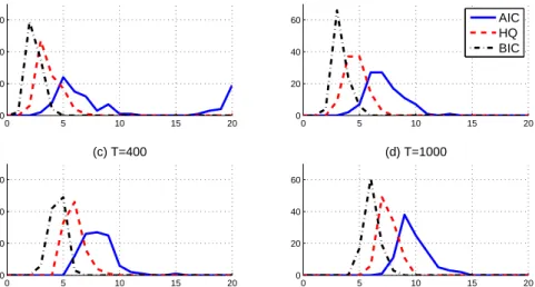
The Johansen procedure is dependent on the lag length of the VECMs, hence we first specify the lag lengths for VARs using the three information criteria. Figure1plots the distribution of the estimated lag length for VARs with different sample sizes. The maximum lag length is set to 20 considering the available sample size. All three of the information criteria choose longer lags as the sample size T increases. AIC has the tendency to choose very long lags when the sample size T = 100. The empirical distributions of the estimated cointegrating rank ˆρ selected by the Johansen procedure

are plotted in Figure2.

Figure 1: Distribution of the estimated lag length for VAR with different sample sizes

0 5 10 15 20 0 20 40 60 (a) T=100 percentage (%) 0 5 10 15 20 0 20 40 60 (b) T=200 AIC HQ BIC 0 5 10 15 20 0 20 40 60 (c) T=400 lag length percentage (%) 0 5 10 15 20 0 20 40 60 (d) T=1000 lag length

It is evident from Figure 2 that the actual size of the Johansen procedure is far from its nominal size of 5%. This phenomenon in finite samples is in accord with the observation byLütkepohl and Saikkonen (1999) when the true DGPs are cointegrated VARMA processes.

Another interesting observation from these two plots is the case when T=100. AIC 7_{A more comprehensive simulation using 100 different DGPs shows that the extendedPoskitt(2000)}

procedure can choose the true cointegrating rank for at least 95% of the time when T = 100. These simulation results are available upon request.

Figure 2: Distribution of the estimated cointegrating rank ˆρwith different sample sizes 1 2 3 0 20 40 60 80 100 (a) T=100 percentage (%) 1 2 3 0 20 40 60 80 100 (a) T=200 AIC HQ BIC 1 2 3 0 20 40 60 80 100 (a) T=400 rank percentage (%) 1 2 3 0 20 40 60 80 100 (a) T=100 rank

chooses very long lags (i.e. higher than 12) more than 20% of the time. In line with the findings ofVahid and Issler(2002), we would expect such an over-parameterization by AIC to cause a large estimation error, especially in small samples. Correspondingly, Figure 2 shows that when T = 100, the Johansen procedure with lag length selected using AIC chooses the correct specification of the cointegrating rank for roughly 60% of the time. This phenomenon also reveals that the cointegrating rank estimated using the Johansen procedure depends crucially on the lag length of the VECM.

Overall, Figures 2 provides supporting evidence in favor of the modified Poskitt (2000) method for choosing the cointegrating rank when the true DGP is a VARMA process. We then proceed to the second stage of the proposed algorithm to identify the underlying SCM structure of each simulated path.

Various studies (see e.g. Athanasopoulos and Vahid, 2008; Athanasopoulos et al., 2012) have found that the identification procedure for specifying the canonical SCM VARMA models is quite successful. We find similar results using the cointegrated VARMA DGP in equation (48). The true SCM structure implied by equation (48) is three SCM(1,1). The testing procedure outlined in Section 3.2 is able to pick up the correct structure for more than 95% of the time. Other identified SCM specifications are listed in AppendixA.

4.2 Forecasting with EC-VARMA models and VECMs

Tables1and2 present the percentage differences in tr(MSFE) and GFESM between the estimated models and the “oracle” at each forecasting horizon. For instance, the first number in Table1denotes that when the sample size is T = 100, the trace of the one-step MSFE obtained from the EC-VARMA models estimated using IOLS is 16.3% larger than the trace of one-step MSFE from the “oracle”. Similar interpretations can be drawn from Table2for GFESM.

T able 1: Per centage dif fer ence in tr(MSFE) for yt in le v els betw een the estimated models and the “oracle” h ECV ARMA AIC HQ BIC ECV ARMA AIC HQ BIC ˆ ρP ˆ ρJ ˆ ρP ˆ ρJ ˆ ρP ˆ ρJ ˆ ρP ˆ ρP ˆ ρJ ˆ ρP ˆ ρJ ˆ ρP ˆ ρJ ˆ ρP T = 100 T = 200 1 16.3 \ 63.1 61.5 28.8 26.2 29.4 28.5 10.7 \ 15.5 16.4 19.6 19.2 21.8 22.2 4 1.0 \ 68.0 51.7 21.1 15.0 7.5 6.1 5.4 \ 21.9 21.1 16.2 12.6 13.1 11.7 8 6.7 \ 76.7 50.4 16.3 12.3 10.5 8.9 6.0 \ 17.0 12.5 15.5 8.3 11.0 7.6 12 10.0 97.3 59.9 11.8 11.4 5.5 \ 9.8 6.7 13.9 7.6 13.0 5.8 \ 9.8 7.7 16 11.2 138.2 77.5 14.6 14.3 8.1 \ 12.6 5.9 15.6 7.8 15.4 5.6 \ 12.2 7.2 20 17.0 175.4 93.1 19.5 17.9 12.9 \ 15.6 8.4 14.6 8.9 14.2 7.4 \ 12.8 8.3 24 18.6 211.3 98.9 21.8 20.8 16.3 \ 18.0 9.7 \ 15.2 10.7 14.3 10.0 14.2 10.0 T = 400 T = 1000 1 5.6 \ 9.0 8.5 11.6 11.1 12.6 12.6 0.8 \ 4.3 4.4 1.7 1.9 5.0 5.1 4 1.8 \ 9.7 11.2 7.5 8.6 4.8 6.3 -2.4 \ 4.5 4.8 3.0 3.2 4.0 3.9 8 3.2 \ 9.8 10.1 7.2 8.0 5.5 5.9 -1.7 \ 2.8 3.6 1.5 2.3 1.4 1.9 12 2.4 \ 7.9 6.6 5.0 4.5 3.1 3.2 -1.7 -0.4 0.2 -2.0 -0.6 -2.6 \ -1.4 16 1.1 \ 8.5 5.3 6.9 4.4 4.1 1.8 -2.9 \ 0.1 0.1 -2.1 -0.4 -2.4 -0.9 20 1.6 \ 8.9 5.2 7.3 4.9 5.2 2.7 -2.2 -0.6 -1.1 -2.3 \ -1.6 -1.3 -1.1 24 2.6 \ 8.3 5.6 5.9 5.3 5.5 3.9 -2.9 \ -0.2 -0.8 -2.2 -1.9 -0.8 -0.6 1ˆρ P : using the cointegrating rank selected b y the extended Poskitt’s method; 2ˆρ J : using the cointegrating rank selected b y the Johansen pr ocedur e; 3\ : indicating the smallest measur e of for ecasting accuracy among the estimated models.

T able 2: Per centage dif fer ence in GFESM betw een the estimated models and the “oracle” h ECV ARMA AIC HQ BIC ECV ARMA AIC HQ BIC ˆ ρP ˆ ρJ ˆ ρP ˆ ρJ ˆ ρP ˆ ρJ ˆ ρP ˆ ρP ˆ ρJ ˆ ρP ˆ ρJ ˆ ρP ˆ ρJ ˆ ρP T = 100 T = 200 1 48.1 \ 185.7 179.3 82.9 75.7 85.3 82.9 29.4 \ 43.8 46.6 57.1 56.0 63.7 65.2 4 46.1 \ 154.6 145.7 54.0 51.4 66.6 66.3 21.4 \ 44.4 44.5 39.9 39.7 50.7 50.7 8 37.2 124.8 116.9 36.2 34.4 \ 45.9 44.9 23.5 \ 30.4 29.1 25.8 24.8 32.3 31.8 12 29.5 106.8 100.7 26.5 25.6 \ 34.5 34.6 18.6 \ 23.4 22.6 20.2 19.8 25.2 25.2 16 25.7 97.2 88.2 20.3 20.2 \ 28.9 28.8 18.6 16.8 16.7 15.1 14.9 \ 19.9 20.1 20 24.1 91.5 83.0 16.1 15.9 \ 24.0 23.6 15.3 15.4 15.8 13.7 13.7 \ 15.3 15.9 24 23.1 87.6 79.6 12.9 \ 13.4 20.0 19.9 14.7 14.0 14.3 11.5 11.1 \ 13.0 13.0 T = 400 T = 1000 1 12.9 \ 24.8 23.5 32.6 31.6 35.5 35.4 -0.8 \ 9.9 10.3 2.0 2.8 12.5 12.9 4 12.6 \ 23.8 24.9 26.8 27.6 29.2 30.2 1.7 \ 16.1 16.5 12.6 12.9 19.8 19.9 8 9.0 \ 22.0 22.1 21.5 21.8 20.1 20.0 1.2 \ 13.7 14.0 12.2 12.4 14.9 15.0 12 8.0 \ 16.8 16.7 15.1 15.3 14.6 14.5 2.0 \ 10.0 10.1 9.3 9.5 10.5 10.7 16 5.5 \ 13.1 13.1 11.3 11.3 11.6 11.2 2.0 \ 8.7 8.7 7.2 7.4 8.0 8.2 20 6.3 \ 12.2 12.3 10.3 10.5 9.5 9.2 0.2 \ 7.2 7.0 6.6 6.4 7.1 6.8 24 7.1 \ 10.5 10.6 9.7 9.6 8.5 8.2 0.6 \ 6.6 6.4 5.6 5.3 5.7 5.4 1ˆρ P : using the cointegrating rank selected b y the extended Poskitt’s method; 2ˆρ J : using the cointegrating rank selected b y the Johansen pr ocedur e. 3\ : indicating the smallest measur e of for ecasting accuracy among the estimated models.

In addition to the estimated EC-VARMA models, we also fit VECMs with lag lengths selected by AIC, HQ or BIC to each simulated data path separately. Conditional on the selected AR lag length, the cointegrating rank is then chosen by the Johansen procedure. VECMs with the cointegrating rank determined by the modifiedPoskitt(2000) approach are also estimated here. The tr(MSFE) and GFESM are reported in Tables1 and2 for both specifications of the cointegrating rank, in columns labeled ˆρJ and ˆρP respectively.

The symbol “\” indicates the model specification that produces the most accurate fore-cast. The evidences provided in Tables 1 and 2 are conclusive, that in general, given the typical sample sizes available for macroeconomic data, using EC-VARMA models reduces the forecasting error, especially with large sample sizes. For small sample sizes, the advantages of EC-VARMA models are quite substantial in short horizons.

The columns labeled ˆρJ and ˆρP in Tables 1 and 2 allow us to examine the effects

on the forecasting accuracy of using different cointegrating ranks. The lag lengths of VECMs are selected by the same information criteria, but the cointegrating ranks are chosen by the Johansen procedure and the extendedPoskitt(2000) method, respectively. The tables show that using the extendedPoskitt(2000) method produces smaller forecast error mostly when the sample size is small.

5

Term Structure of Interest Rates

It is commonly accepted that interest rates with different maturities are cointegrated (see Hall et al., 1992). The cointegrating vector between any two interest rate series should be close to (1,−1),i.e. the interest rate spreads should be stationary, despite the fact that most interest rates are regarded as I(1) series. Many studies of interest rates have been conducted within the VECM framework, with the aim of forecasting interest rates. To name one among others, Hall et al.(1992) find that yields to maturity of U.S. treasury bills specify an error correction model with post-1982 data, which proves to be useful in forecasting changes in yields.

The use of VARMA models to capture the dynamics in the term structure of interest rates is not new. Kascha and Trenkler (2011) show that a cointegrated VARMA model generates superior forecasts of U.S. interest rates. Nevertheless, our study differs from theirs in several aspects. First, Kascha and Trenkler (2011) extend the FMA represen-tation of Dufour and Pelletier (2008) to specify their VARMA model. This is simpler but less general and parsimonious than the SCM representation (Athanasopoulos and Vahid,2008) employed here. Moreover,Kascha and Trenkler(2011) take the cointegrat-ing rank as given (ρ = K−1) for their forecasting evaluation, whereas we test for the

cointegrating rank for each sample.

5.1 Data

We use monthly data of the U.S. federal funds rate, and 3-month and 6-month treasury bill rates to form a three variable system. Let yt = (f ft,i3t,i6t)0. The available sample

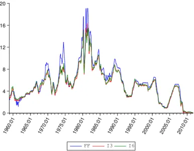
period is from 1958:12 to 2011:09, which leads to a total of 634 observations. Figure

3 plots the three interest rate series over the entire sample period. The movements in the three series clearly share a similar pattern, especially for the 3-month and 6-month treasury bill rates.8

Figure 3: The three interest rate series (%)

0 4 8 12 16 20 1960:01 1965:01 1970:01 1975:01 1980:01 1985:01 1990:01 1995:01 2000:01 2005:01 2010:01 FF I3 I6

We use the first 400 observations as the initial estimation sample to forecast future interest rates for up to 12-steps ahead. We use an expanding window,9 and the same forecasting exercise is repeated 222 times. In addition to tr(MSFE) for yt in levels and

GFESM, the determinant of MSFE (det(MSFE)) for yt in levels is also examined.

5.2 Selection of Cointegrating Rank and Lag Length

We first estimate the VECMs and EC-VARMA models using the theoretical cointegrating relationships — for a K-dimensional model, the cointegrating rank is fixed to be ρ =

K−1. Furthermore, the cointegrating vectors are specified as follows:

β= h 1, −1, 0 0 , 1, 0, −1 0i . (50)

The AR order of the finite VAR is determined using AIC, HQ and BIC. The maximum AR lag is set to be 24 which is two years for monthly data. The distributions of the 8_{One may want to drop the observations during the last global financial crisis (2008:01-2011:09, the last}

45 observations), due to the possibility of a structural break. We experiment with this shorter sample as well, and it produces qualitatively similar results. The forecast errors are smaller in almost all cases, but the ranking of the competing models does not change.

9_{We also use rolling window to generate forecasts of future interest rates, which can account for the}

possible structural breaks over the time span that we considered. The forecasting results are very similar to what are reported below using expanding window, and hence are omitted here. Those results are available upon request.

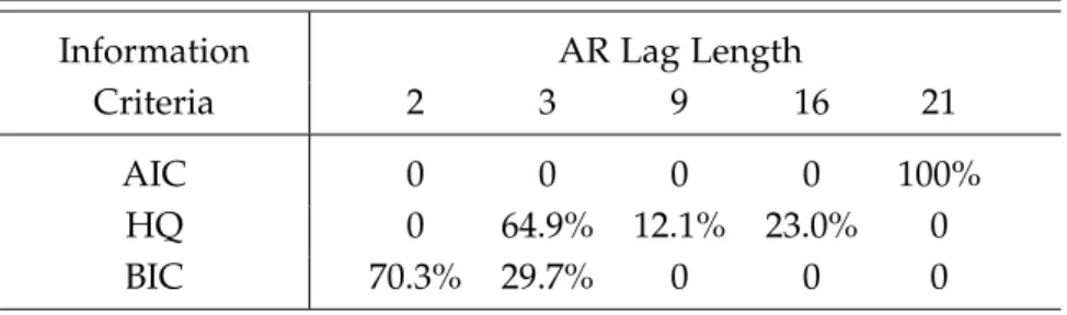
selected AR lag length for 222 sets of estimation samples are tabulated in Table3. All of the models specified by AIC are heavily parameterized, choosing a VAR(21) for yt

in levels for all 222 sets of estimation samples. BIC seems to choose a much shorter lag length for this dataset. Surprisingly, HQ only chooses three different lag lengths — 3, 9 and 16, which do not increase gradually, but this is what is observed from the data using an expanding window.

Table 3: Distribution of the estimated lag length for VAR with theoretical cointegration

Information AR Lag Length

Criteria 2 3 9 16 21

AIC 0 0 0 0 100%

HQ 0 64.9% 12.1% 23.0% 0

BIC 70.3% 29.7% 0 0 0

Table 4: Distribution of the estimated lag length and cointegrating rank (data-specified cointegration) Information

Lag Cointegration Rank

Criteria 0 1 2 AIC 21 48.2% 51.8% HQ 3 64.9% 9 0.9% 11.3% 16 23.0% BIC 2 70.3% 3 29.7% Poskitt’s Method 100%

Empirical researchers usually estimate the cointegrating relationships from the data rather than fix them beforehand. Thus, we also investigate the forecasting performances of models with data-specified cointegration. We use the algorithm proposed in Section

3 to identify the structure of the EC-VARMA models. The first step of the procedure determines the cointegrating rank. The extended non-parametric approach (Poskitt, 2000) applied to this three variable system chooses ˆρ = 2 consistently for all 222 sets

of estimation samples. On the other hand, the Johansen procedure chooses different cointegrating ranks based on the lag lengths selected by different information criteria. The lag length and cointegrating rank specified by the two methods are tabulated in Table4. AIC once again shows a tendency toward over-parameterization. The joint use of the Johansen procedure and AIC chooses ˆρ = 0 or ˆρ = 1. Neither of these comply

with economic theory. VECM with lag length selected using BIC chooses a reasonable lag length and an expected cointegrating rank ˆρ =2.

5.3 Canonical SCM VARMA Representation

There is no evidence in the literature showing that a system of interest rates follows a VARMA process. Hence, the second stage of identifying the VARMA model is necessary in order to justify the choice of this model. We use the SCM methodology to determine the lag orders and the corresponding canonical structure of the VARMA model, keeping in mind that even if the true DGP is a finite order VAR process, the SCM searching procedure is able to identify a VARMA(p,0) model asymptotically.

Conditional on the identified tentative overall order VARMA(1,1) for yt in levels,

we search for each individual SCM. Starting from the most parsimonious SCM(0,0), the underlying SCMs are identified as SCM(1,1)∼ SCM(1,1)∼ SCM(1,0). After testing the SCM structure of the sub-systems and imposing identification restrictions on Φ0 (see

Athanasopoulos, 2007; Athanasopoulos and Vahid, 2008), the canonical SCM VARMA model has the following error correction representation:

   1 0 0 0 1 0 a0 0 1   ∆yt =    α11 α12 α21 α22 α31 α32       1 β12 β21 1 β31 β32    0 yt−1+ut+    θ1₁₁ θ1₁₂ θ₁₃1 θ1₂₁ θ1₂₂ θ₂₃1 0 0 0   ut−1. (51)

We find exactly the same SCM structure for all 222 sets of estimation samples. There are no zero restrictions imposed on Φ1 by the canonical SCM structure. Hence, the rank

restrictions on Π only come from the cointegration relationships. We estimate equation (51) using FIML. In order to provide good initial estimates for maximum likelihood estimation, we put the algorithm ofHannan and Rissanen(1982) into the context of EC-VARMA models, as the starting values of the unknown parameters for the maximum likelihood iteration. This initial estimate works well for this empirical example. The model structure in equation (51) is also used for the estimation with the theoretical cointegrating vectors.

5.4 Forecast Evaluation of Interest Rates

The measures of forecasting accuracy calculated from all types of models are presented in Table5. We take the EC-VARMA model with theoretical cointegration relationships as the benchmark. The first three columns are models with theoretical cointegration relationships, and the last four columns are models with data-specified cointegration, denoted by the subscript “d”. It is worth reminding ourselves that the modified Poskitt’s method always chooses a cointegrating rank of ˆρ = 2 = K−1. Hence, the only

differ-ence between SCMd and the benchmark model in this application is due solely to the

Table 5: Percentage difference in measures of forecast accuracy between other models and the EC-VARMA models with theoretical cointegration

Theoretical Data-specified

Cointegration Cointegration

VECMs VECMs

SCMd

h AIC HQ BIC AICd HQd BICd

tr(MSFE) 1 56.6 31.5 14.7 59.0 33.1 16.3 0.9 4 40.1 12.1 6.1 43.1 13.8 5.1 3.8 8 23.0 1.8 3.8 21.3 6.8 4.7 6.9 12 17.8 −1.1\ 4.4 11.9 5.6 6.0 7.3 det(MSFE) 1 112.4 52.0 17.7 118.9 54.7 28.8 −4.8\ 4 72.4 35.3 16.9 85.4 25.5 14.6 −22.6\ 8 20.0 16.7 17.0 37.2 1.9 1.5 −35.8\ 12 −0.0 0.8 16.5 14.5 −26.4 −19.9 −48.9\ GFESM 1 112.4 52.0 17.7 118.9 54.7 28.8 −4.8\ 4 101.5 39.0 6.2 105.2 36.4 6.2 −6.9\ 8 97.9 29.9 2.0 99.7 29.2 1.0 −3.9\ 12 90.3 23.9 0.8 23.8 23.8 −0.0 −2.2\

\: indicates the smallest measure of forecasting accuracy in each row.

The numbers in Table5 indicate the percentage by which the measures of forecast-ing accuracy calculated from each type of model are larger than the measures calculated from the benchmark model. Hence, a negative number indicates an improvement in forecasting accuracy over EC-VARMA model with theoretical cointegration on average. The symbol “\” denotes the type of model that produces the smallest measure of fore-casting accuracy in each row. No “\” in a row indicates that the benchmark model is most accurate.

In Table 5, VECMs with lag lengths chosen using AIC usually lead to the largest forecast error. Such results are not surprising, taking into account the presumably large estimation error caused by the over-parameterization of AIC. It is evident that if the theoretical cointegrating relationships are imposed, EC-VARMA models have smaller tr(MSFE) than VECMs in most of the scenarios considered here. Their advantages over VECMs are more pronounced in the short run. EC-VARMA models with data-specified cointegrating vectors generate the smallest det(MSFE) and GFESM of all of the different model specifications up to 12-step ahead forecasts. In terms of the determinant of the MSFE, there are considerable gains from estimating the cointegrating vectors from the

data rather than using the theoretical ones. The values of det(MSFE) can be reduced by nearly 50% by the use of the EC-VARMA models with estimated cointegrating vectors. The other two measures calculated from the EC-VARMA models with either estimated or theoretical cointegrating relationships are of roughly the same sizes.

5.5 Diebold-Mariano Tests

One may be concerned about the importance of the results reported in Tables 5, since most of the differences between these measures of forecasting accuracy generated from VECMs and EC-VARMA models are very small in magnitude. We use the Diebold-Mariano test (Diebold and Mariano, 1995; West, 1996; Giacomini and White, 2006) to compare the predictive accuracies of these two classes of models. The hypotheses are

H0:E e2_1,i,h −E e2_2,i,h =0, against H1:E e2_1,i,h −E e2_2,i,h <0, (52) where e1,i,h and e2,i,h denote the h-step ahead forecast errors of the i-th component

of yt, generated from the estimated EC-VARMA model and VECMs, respectively, with

i = 1, 2, 3. The forecast errors of fft, i6t and i3t are te