Misspecification Testing in a Class of Conditional Distributional Models

D I S C U S S I O N P A P E R S E R I E S Forschungsinstitut zur Zukunft der Arbeit

Misspecification Testing in a Class of

Conditional Distributional Models

February 2012 Christoph Rothe Dominik Wied

Misspecification Testing in a Class of

Conditional Distributional Models

Christoph Rothe

and IZA

Dominik Wied

Discussion Paper No. 6364

February 2012

Anyopinions expressed here are those of the author(s) and not those of IZA. Research published in this series may include views on policy, but the institute itself takes no institutional policy positions. The Institute for the Study of Labor (IZA) in Bonn is a local and virtual international research center and a place of communication between science, politics and business. IZA is an independent nonprofit organization supported by Deutsche Post Foundation. The center is associated with the University of Bonn and offers a stimulating research environment through its international network, workshops and conferences, data service, project support, research visits and doctoral program. IZA engages in (i) original and internationally competitive research in all fields of labor economics, (ii) development of policy concepts, and (iii) dissemination of research results and concepts to the interested public. IZA Discussion Papers often represent preliminary work and are circulated to encourage discussion.

IZA Discussion Paper No. 6364 February 2012

ABSTRACT

Misspecification Testing in a Class of

Conditional Distributional Models

We propose a specification test for a wide range of parametric models for the conditional distribution function of an outcome variable given a vector of covariates. The test is based on the Cramer-von Mises distance between an unrestricted estimate of the joint distribution function of the data, and a restricted estimate that imposes the structure implied by the model. The procedure is straightforward to implement, is consistent against fixed alternatives, has non-trivial power against local deviations of order n-1/2 from the null hypothesis, and does not require the choice of smoothing parameters. In an empirical application, we use our test to study the validity of various models for the conditional distribution of wages in the US.

JEL Classification: C12, C14, C31, C52, J31

Keywords: Cramer-von Mises distance, quantile regression, distributional regression, location-scale model, bootstrap, wage distribution

Corresponding author:

Christoph Rothe

Toulouse School of Economics

Manufacture des Tabacs, Office MF 404 21 Allée de Brienne

31000 Toulouse France

E-mail: [email protected]

1. Introduction

In this paper, we propose a general principle to construct omnibus specification test for a wide range of parametric models for a conditional distribution function. For Y ∈_Ran outcome variable andX ∈_RK _{a vector of covariates, our interest is in testing the validity}

of a model that asserts that there exists a possibly function-valued parameter θ = θ(·) such that

Pr(Y ≤y|X =x) = F(y|x, θ) for all (y, x)∈ Z, (1.1)

whereF(·|·, θ) is a known function andZ denotes the support ofZ = (Y, X). We refer to any such specification as a conditional distributional model. The alternative hypothesis is that equation (1.1) is violated for at least one value (y, x) ∈ Z. Allowing unknown parameters to be function-valued is important in this setting, and constitutes one of the main innovations of our approach. We also discuss an extension of our procedure that allows to test the hypothesis in (1.1) for all (y, x) in some set S ⊂ Z chosen by the analyst. Through an appropriate choice of S one can test whether the parametric model provides an adequate fit over a particular range of the conditional distribution function, such as e.g. the area below or above the conditional median.

Our general setting covers a wide range of conditional distributional models that are of great importance in empirical applications. The leading example is certainly thelinear quantile regression model (Koenker and Bassett, 1978; Koenker, 2005), which implies a linear structure for the inverse of the conditional CDF, namely that F−1_{(τ|x, θ) = x}0_θ(τ)

for some functional parameter θ(·) that is strictly increasing in each of its components. Nonlinear versions of quantile regression could be considered as well. Another example is thelinear location-scale shift model (Koenker and Xiao, 2002), under whichF−1_{(τ|x, θ) =} x0β +x0γQ(τ), with Q a univariate quantile function and θ(·) = (β, γ, Q(·)). We

also cover the distributional regression model (Foresi and Peracchi, 1995), where the conditional CDF is modeled by a series of binary response models with varying “cutoffs”. That is, the conditional CDF is specified as F(y|x, θ) = Λ (x0θ(y)), where Λ is a known strictly increasing link function such as e.g. the logistic or standard normal distribution function, and θ(·) is again a function-valued parameter. This latter class of models has

recently received considerable attention in the econometrics literature (e.g. Chernozhukov, Fernandez-Val, and Melly, 2009; Fortin, Lemieux, and Firpo, 2011; Koenker, 2010; Rothe, 2011).

Our test is an extension of the method proposed by Andrews (1997) in the context of parametric models indexed by finite dimensional parameters. The basic idea is to compare an unrestricted estimate of the joint distribution function of Y and X to a restricted estimate that imposes the structure implied by the conditional distributional model. For example, to test the validity of the linear quantile regression model we would first obtain an estimate of the conditional CDF of Y givenX by inverting the estimated conditional quantile function, and then transform this object into an estimate of the joint CDF of (Y, X) by “integrating up” the conditioning argument. This restricted CDF estimate can then be compared to the joint empirical distribution function of (Y, X).

Our test statistic is a Cramer-von Mises type measure of distance between the two above-mentioned objects, and is therefore called a Generalized Conditional Cramer-von Mises(GCCM) test.1 We reject the null hypothesis that the parametric model is correctly specified whenever this distance is “too large”. Since our test statistic is not asymptoti-cally pivotal, critical values cannot be tabulated, but can be obtained via the bootstrap. While our test is thus computationally somewhat involved, it is straightforward to im-plement and has a number of attractive theoretical properties: It is consistent against all fixed alternatives, has non-trivial power against local deviations from the null hypothe-sis of order n−1/2 (where n denotes the sample size), and does not require the choice of smoothing parameters.

The correct specification of conditional distributional models of the type considered in this paper is critical in many areas of applied statistics. In economics, such specifications are e.g. employed extensively to study differentials in the distribution of wages between two time periods, or two subgroups of a particular population. See e.g. Machado and Mata (2005), Melly (2005), Albrecht, Van Vuuren, and Vroman (2009), Chernozhukov et al. (2009) or Rothe (2011), and Fortin et al. (2011) for an extensive survey. From a

1_{We choose to work with the CvM distance instead of other measures, such as e.g. the Kolmogorov}

distance used by Andrews (1997), since the resulting test statistics turned out to have substantially better power properties in simulations. This is in line with classical findings on the power of specification tests, e.g. Stephens (1974).

statistical point of view, these methods first obtain an estimate of the conditional CDF of Y given X. In a second step, this function is integrated with respect to another CDF, whose exact form depends on the particular application, yielding a new univariate distribution function. As a final step, features of this new distribution function, such as its mean or quantiles, are computed. Our concern is the implementation of the first step of this procedure. For example, the Machado and Mata (2005) decomposition procedure relies on the assumption that theentire conditional distribution of wages given observable individual characteristics can be described by a linear quantile regression model. If this assumption is violated, the method can potentially lead to inappropriate conclusions (see Rothe, 2010, for some simulation evidence). From a practitioner’s point of view, misspecification is a serious concern in this context, as the conditional quantiles of the wage distribution are e.g. known to be extremely flat in the vicinity of the legal minimum wage, and might thus not be described adequately by a linear specification in this region (Chernozhukov et al., 2009). Our testing procedure can be used to formally investigate this issue.

As an additional contribution, our paper provides some empirical evidence on the last point: using US data from the Current Population Survey, we show that typical specifications of linear location-scale models and linear quantile regressions containing a rich set of covariates are frequently rejected by our GCCM test even for small and moderate sample sizes. On the other hand, we find that the distributional regression model, which has thus far received only limited interest in the literature, typically cannot be rejected in such settings. The finding should have a profound impact on the way researchers model conditional wage distributions in practice, particularly in the context of decomposition exercises. It should also renew interest in distributional regression model, whose statistical properties are not yet fully understood (see Koenker (2010) for some basic results).

There exists an extensive literature on specification testing in parametric models for the conditional expectation function (see e.g. Bierens, 1990, H¨ardle and Mammen, 1993, Bierens and Ploberger, 1997, Stute, 1997 and Horowitz and Spokoiny, 2001), and for the conditional quantile function atone particular quantile, such as the median (see e.g. Zheng, 1998, Bierens and Ginther, 2001, Horowitz and Spokoiny, 2002, He and Zhu, 2003,

and Whang, 2006). In comparison, the related problem of testing the validity of a model for the entire conditional distribution function that we study in this paper has received much less attention. Andrews (1997) proposes a test for conditional distributional mod-els indexed by finite-dimensional parameters, such as e.g. Generalized Linear Modmod-els, which we extend in this paper as described above. Koenker and Machado (1999) and Koenker and Xiao (2002) consider specification testing in a quantile regression context, and propose tests for e.g. the validity of the location-scale model, but not the validity of the quantile regression model itself. Galvao, Kato, Montes-Rojas, and Olmo (2011) test for threshold effects in linear quantile regression in a time series context. Escanciano and Velasco (2010) and Escanciano and Goh (2010) both propose testing procedures for the null hypothesis that a conditional quantile restriction is valid over a range of quan-tiles. The former paper considers specification testing for dynamic quantile regression models in a time series setting using a subsampling approach, whereas the latter paper studies the instrumental variables quantile regression model of e.g. Chernozhukov and Hansen (2005), obtaining critical values via a multiplier bootstrap scheme. The settings of these two papers are thus very different from ours in general, but include the usual quantile regression model with independent observations as a special case. We are not aware of any paper that provides a general approach to testing the validity of conditional distributional models indexed by possibly function-valued parameters.

The remainder of the paper is structured as follows. In the next section, we describe our testing problem, the test statistic, and a bootstrap procedure to obtain critical values. In Section 3, we establish the theoretical properties of our test under general conditions. In Section 4, we apply these general results to several concrete examples. Section 5 dis-cusses an extension of our test procedure that allows to check the model’s validity for some particular part of the conditional CDF. Section 6 contains some Monte Carlo evidence on the finite sample properties of our test, and Section 7 evaluates the appropriateness of various models for the conditional distribution of wages given individual characteristics in the US. Finally, Section 8 concludes.

2. Testing General Conditional Distributional Models

2.1. Testing Problem. We observe an outcome variable Yi ∈ R and a vector of

explanatory variables Xi ∈ RK for i = 1, . . . , n. The random vector Zi = (Yi, Xi) has a

joint cumulative distribution function (CDF) H, and its random subcomponent Xi has

joint CDF G. We assume throughout the paper that the data points are independent and identically distributed, although it would also be possible to extend our analysis to certain forms of temporal dependence. Our aim is to test the validity of certain classes of parametric specifications for the conditional CDFF of Yi givenXi. LetF be the class

of all conditional distribution functions on the support of Y given X that satisfy certain weak regularity conditions given below, and consider a conditional distributional model, i.e. a parametric family

F0 _{={F(·|·, θ) for someθ ∈ B(T,Θ)} ⊂ F}

of conditional distribution functions indexed by a (potentially) functional parameter θ taking values in B(T,Θ), the class of mappings u 7→ θ(u) such that θ(u) ∈ Θ⊂ _Rp _for

u∈ T ⊂_R. The hypothesis we would like to test is that F coincides with an element of

F0_:

H0 :F(y|x) = F(y|x, θ) for some θ∈ B(T,Θ) and all (y, x)∈ Z (2.1) vs. H1 :F(y|x)6=F(y|x, θ) for all θ ∈ B(T,Θ) and some (y, x)∈ Z. (2.2)

This paper proposes a testing procedure of the problem in (2.1)–(2.2) for conditional distributional models in which the true value of the functional parameter is identified under the null hypothesis through a moment condition. Specifically, let ψ : Z ×Θ× T 7→ _Rp _{be a uniformly integrable function whose exact form depends on the specific}

conditional distributional model F0_{, and suppose that for every u∈ T the equation}

Ψ(θ, u) :=_E(ψ(Z, θ, u)) = 0 (2.3)

θ ∈ B(T,Θ) of the functional parameter that satisfiesF(y|x) =F(y|x, θ) for all (y, x)∈ Z also satisfies θ(u) = θ0(u) for all u ∈ T. The moment condition (2.3) thus uniquely de-termines the value of the “true” functional parameter. Under the alternative, θ0 remains well-defined as the solution to (2.3), and can thus be thought of as a pseudo-true value of the functional parameter in this case. Condition (2.3) also suggests that θ0(u) can be estimated by a Z-estimator.

The class of conditional distributional models that satisfy the above conditions con-tains a number of important specifications that are frequently used in applied work. It e.g. includes the scale-location shift model, quantile regression, and distributional regres-sion, amongst many others. We illustrate how these examples fit into our framework in more detail in Section 4. General results on estimation and inference in this class of mod-els are derived in Chernozhukov et al. (2009). Their findings are important for the later technical arguments in this paper. When the parameter θ0 =θ0(u) does not depend on u the framework also includes many limited dependent variable models and generalized linear models.

2.2. Test Statistic. To motivate our test statistic for the problem in (2.1)–(2.2), we rewrite the null hypothesis and the alternative in a slightly different form. Following the above discussion, it is clear that (2.1) is equivalent to the statement that

F(y|x) = F(y|x, θ0) for all (y, x)∈_RK+1, (2.4)

withθ0(u) the unique solution to (2.3), since by assumptionF(·|·, θ0) is the only element of F0 _{that is a potential candidate value for the true conditional CDF F of Y}

i givenXi.

Equation (2.4) is a conditional moment restriction, that can equivalently be stated as

E(I{Y ≤y} −F(y|x, θ0)|X =x) = 0 for all (y, x)∈RK+1. (2.5)

Using a result from Billingsley (1995, Theorem 16.10(iii)), this conditional moment re-striction can be transformed into an unconditional one without loss of information by

“integrating up” with respect to x: statement (2.5) is true if and only if

R(y, x) := _E((_I{Y ≤y} −F(y|X, θ0))I{X ≤x}) = 0 for all (y, x)∈RK+1.

Note that the same approach it also used in e.g. Stute (1997) for testing parametric specifications of conditional expectation functions. The function R(y, x) has an intuitive interpretation as the pointwise distance between the joint CDF

H(y, x) =P(Y ≤y, X ≤x) of (Y, X) and another CDF H0(y, x) = Z t≤x F(y|t, θ0)dG(t)

that imposes the structure implied by the conditional distributional model. To see this, note that it follows from the Law of Iterated Expectations that

R(y, x) = Z t≤x F(y|t)dG(t)− Z t≤x F(y|t, θ0)dG(t) =:H(y, x)−H0(y, x).

With the above notation, our testing problem (2.1)–(2.2) is equivalent to

H0 :R(y, x) = 0 for all (y, x)∈_RK+1 vs. H1 :R(y, x)6= 0 for some (y, x)∈_RK+1.

A test statistic for this problem can then be constructed from an empirical analogue of the function R(y, x), given by

b Rn(y, x) = 1 n n X i=1 (_I{Yi ≤y} −Fb_n(y|X_i))I{X_i ≤x}=:Hb_n(y, x)−Hb_n0(y, x).

Here Fbn(y|x) = F(y|x,θb_n) is a parametric estimate of F based on an estimate θb_n of θ0, and thus Rb_n(y, x) is the pointwise difference between the joint empirical distribution

function b Hn(y, x) =n−1 n X i=1 I{Yi ≤y, Xi ≤x}

and the semiparametric CDF estimate

b H_n0(y, x) =n−1 n X i=1 b Fn(y|Xi)I{Xi ≤x}.

We take θb_n to be an approximate Z-estimator satisfying

kΨbn(θb_n(u), u)k=o_p(n−1/2),

where Ψb_n(θ, u) := n−1

Pn

i=1ψ(Zi, θ, u) is the sample analogue of the moment condition

in (2.3). Such an approach is feasible for all examples we consider in this paper.

Under general conditions described in the following section, the random process (y, x) 7→ Rb_n(y, x) converges to zero in probability under the null hypothesis, and to a non-zero probability limit under the alternative. One can thus construct a specifica-tion test for the condispecifica-tional distribuspecifica-tional model F0 _{based on a Cramer-von Mises type} measure of distance betweenRb_nand zero, scaled by the sample size. Specifically, the test statistic Tn is defined as:

Tn=n Z b Rn(y, x)2dHbn(y, x) = n X i=1 b Rn(Yi, Xi)2.

Large realizations of Tn indicate a possible violation of the null hypothesis. Since our

testing principle shares some similarity with the Conditional Kolmogorov2test in Andrews (1997), we refer to our test in the following as a Generalized Conditional Cramer-von Mises (GCCM) test.

2_{The reason for departing from Andrews (1997) with respect to the distance measure is that our}

simulation experiments suggested that Cramer-von Mises type statistics have somewhat better power properties than those based on the Kolmogorov distance. It would of course conceptionally be straight-forward to consider other measures of distance betweenRbn and zero to construct a test statistic for the

problem in (2.1)–(2.2). The properties of such a test could be derived in exactly the same way as the one presented in the following subsections.

2.3. Bootstrap Critical Values. As we show in more detail below, for most common conditional distributional models the null distribution of Tn is non-pivotal and depends

on the data generating process in a complex fashion. We therefore obtain critical values for our test statistic by a semiparametric bootstrap procedure, using the restricted es-timate Hb_n0 as the bootstrap distribution. Since Fbn ∈ F0 by construction, this approach

ensures that the bootstrap mimics the distribution of the data under the null hypothesis, even though the data might be generated by an alternative distribution. A bootstrap realization of our test statistic is computed as follows:

Step 1: Draw a bootstrap sample of covariates {Xb,i,1≤i≤n} with replacement from

the realized values {Xi,1≤i≤n}.

Step 2: For every 1 ≤ i ≤ n put Yb,i = Fb_n−1(Ub,i|Xb,i), where {Ub,i,1 ≤ i ≤ n} is a

simulated i.i.d. sequence of standard uniformly distributed random variables.

Step 3: Use the bootstrap data{(Yb,i, Xb,i),1≤i≤n}to compute an estimateRbb,n(y, x)

of R(y, x) exactly as described in the previous subsection, and compute the corre-sponding bootstrap realization of the test statistic:

Tb,n=n Z

b

Rb,n(y, x)2dHb_n(y, x).

The distribution of Tb,n can be determined through the usual repeated resampling of the

data, and, as shown formally below, then be used as an approximation to the distribution ofTnunder the null hypothesis for a wide range of conditional distributional models. An

asymptotically valid level αcritical value _bcn(α) for the testing problem in (2.1)–(2.2) can

be obtained by computing the (1−α)-quantile of the distribution ofTb,n, i.e.bcn(α) is the smallest constant that satisfies

Pb(Tb,n ≤bcn(α))≥1−α,

wherePb is the probability with respect to bootstrap sampling. The test thus rejectsH0 if Tn >bcn(α) for some pre-specified significance level α∈(0,1).

3. Theoretical Properties

This section shows that the GCCM test has correct asymptotic size, consistency against fixed alternatives, and non-trivial power against local deviations from the null hypothesis of order n−1/2_{. We write “→” to denote convergence in distribution of a sequence of}d random variables, and “⇒” to denote weak convergence of a sequence of random func-tions. In addition, we write “the data are distributed according toFe” whenever the joint distribution function ofZ = (Y, X) is given byHe(y, x) =

R e

F(y|t)_I{t≤x}dG(t) for some e

F ∈ F, and denote the expectation taken with respect to any such CDF He by E

e

H. All

limits are taken asn → ∞.

3.1. Limiting Distribution of the Test Statistic. To derive large sample properties of our test statistic we impose the following assumptions.

Assumption 1. The set Θ is a compact subset of _Rp _{and T is either a finite subset or}

a bounded open subset of _R.

Assumption 2. For each u ∈ T, there exists a unique value θ0(u) in the interior of Θ

such that Ψ(θ0(u), u) = 0.

Assumption 3. The mapping (θ, u) 7→ ψ(Z, θ, u) is continuous at each (θ, u) ∈ Θ×T

with probability one, and continuously differentiable at(θ0(u), u)with a uniformly bounded derivative on T (where differentiability in u is only required when T is not finite). The function Ψ(˙ θ, u) :=∂θΨ(θ, u) is nonsingular at θ0(·) uniformly in u∈T.

Assumption 4. The set of functions G ={ψ(Z, θ, u),(θ, u)∈Θ×T} isH-Donsker with a square integrable envelope.

Assumption 5. The mappingθ 7→F(·|·, θ)is Hadamard differentiable at allθ∈ B(T,Θ), with derivative h7→F˙(·|·, θ)[h].

Assumptions 1–4 are standard regularity conditions also imposed by Chernozhukov et al. (2009). They ensure that a functional central limit theorem can be applied to the Z-estimator process u 7→ √n(ˆθn(u)−θ0(u)), and thus that this process converges to a Gaussian limit as n tends to infinity. Assumption 5 is a smoothness condition that

can be verified directly in applications. Together with the Functional Delta Method, it implies that the restricted CDF estimator process (y, x) 7→ √n(Hb_n0(y, x)−H0(y, x)) also converges to a Gaussian limit process _G2. This convergence can be shown to be jointly with that of the empirical CDF process (y, x) 7→ √n(Hb_n(y, x)−H(y, x)) to an H-Brownian Bridge _G1. Since Rbn(y, x) = Hbn(y, x)−Hb_n0(y, x), the limiting distribution of our test statistic Tn follows from an application of the continuous mapping theorem,

and from the fact that the functions H and H0 coincide under the null hypothesis, but differ on a set with positive probability under the alternative.

Theorem 1. Under Assumption 1–5, the following statements hold.

i) Under the null hypothesis, i.e. when the data are distributed according to some F

that satisfies (2.1), Tn d → Z (_G1(y, x)−G2(y, x)) 2 dH(y, x),

where_G= (_G1,G2)is a bivariate mean zero Gaussian process given in the Appendix.

ii) Under any fixed alternative, i.e. when the data are distributed according to some F

that satisfies (2.2),

lim

n→∞P(Tn > c)→1 for all constants c >0.

3.2. Local Alternatives. This section derives the limiting distribution of our test statistic under a sequence of local alternatives that shrink towards an element of F0 _at raten−1/2_{, wherendenotes the sample size. That is, the conditional distribution function} of Y given X is given by

Qn(y|x) = (1−δ/

√

n)F∗(y|x) + (δ/√n)Q(y|x), (3.1)

whereF∗is a CDF such thatF∗(y|x) =F(y|x, θ) for someθ∈ B(T,Θ) and all (y, x)∈ Z, Q is a CDF such that Q(y|x)6= F(y|x, θ) for all θ ∈ B(T,Θ) and some (y, x)∈ Z, and δ≤n1/2 is some constant, satisfying the following assumption.

Assumption 6. The sequence Hn(y, x) = R

Qn(y|t)I{t ≤x}dG(t) of distribution

func-tions implied by the local alternative Qn given in (3.1) is contiguous to the distribution

function H∗(y, x) =R

F∗(y|t)_I{t ≤x}dG(t) implied by F∗.

The requirement that the local alternatives are contiguous (see e.g. Van der Vaart, 2000, Section 6.2 for a formal definition of contiguity) to the limiting distribution function is standard when analyzing local power properties. When the conditional distribution functions F∗ and Q admit conditional density functions f∗ and q with respect to the sameσ-finite measure (e.g. the Lebesgue measure), respectively, a sufficient condition for contiguity is

sup (x,y):f∗_(y|x)>0

q(y|x)

f∗_(y|x) <∞. (3.2)

Intuitively, this would be the case when Q has lighter tails than F∗. This statement is formally proven in Section B in the Appendix.

The following theorem shows that under local alternatives of the form (3.1) the limiting distribution of Tn contains an additional deterministic shift function

ensur-ing non-trivial local power of the test. To describe this function, define ΨQ(θ, u) =

EQ(ψ(Z, θ, u)) and Ψ∗(θ, u) =EF∗(ψ(Z, θ, u)), and let θ_Q and θ_∗ be the functions

satis-fying ΨQ(θQ(u), u) = 0 and Ψ∗(θ∗(u), u) = 0 for all u∈T, respectively.

Theorem 2. Under Assumption 1–6, and if the data are distributed according to a local alternative Qn as given in (3.1), Tn d → Z (_G1(y, x)−G2(y, x) +µ(y, x)) 2 dH(y, x). where µ(y, x) =δ Z Q(y|t)−F(y|t, θ∗) + ˙F(y|t, θ∗) [h] I{t≤x}dG(t) with h(u) =∂θ0Ψ_F∗(θ_∗(u), u)−1Ψ_Q(θ_∗(u), u).

Note that the function F∗ to which the local alternative Qn shrinks can be

ΨQ(θ∗(u), u) = 0 for all u∈T, and hence the drift term in Theorem 2 simplifies to

µ(y, x) =δ Z

(Q(y|t)−F(y|t, θ∗))I{t ≤x}dG(t),

and is thus proportional to the difference between the joint distribution functions implied byQ and F∗.

3.3. Validity of the Bootstrap. As a final step, we establish asymptotic validity of the critical values obtained via the bootstrap procedure described in Section 2.3. This does not require any further assumptions. Under the null hypothesis, Assumptions 1– 5 ensure that the bootstrap consistently estimates the limiting distribution of the test statistic Tn, and hence consistently estimates the true critical values. Under any fixed

alternative, the bootstrap critical values can be shown to be bounded in probability. Together with Theorem 1(ii), this implies that the power of our test converges to one in this case. Finally, since contiguity preserves convergence in probability, it follows from Assumption 6 that under any local alternative the bootstrap critical values converge to the same value as under the null hypothesis. We can thus deduce from Anderson’s Lemma that our test has non-trivial local power. The following theorem formalizes these arguments.

Theorem 3. Under Assumption 1–6, the following statements hold for any α∈(0,1): i) Under the null hypothesis, i.e. when the data are distributed according to some CDF

F that satisfies (2.1), we have that

lim

n→∞P (Tn>bcn(α)) =α.

ii) Under any fixed alternative, i.e. when the data are distributed according to some CDF

F that satisfies (2.2), we have that

lim

n→∞P (Tn >bcn(α)) = 1.

CDF Qn that satisfies (3.1), we have that

lim

n→∞P (Tn>bcn(α))≥α.

4. Application to Specific Models

In this subsection, we discuss a number of conditional distributional models whose correct specification can be investigated via our GCCM test. We also provide primitive condi-tions that imply the “high-level” condicondi-tions in Assumption 1–5 that we used to derive asymptotic properties.

4.1. Quantile Regression. Arguably the most important example of a conditional distributional model indexed by function-valued parameters in the sense of this paper is the linear quantile regression model (Koenker and Bassett, 1978; Koenker, 2005). It postulates that the conditional τ-quantile of Y given X = x is linear in a vector of parameters that vary with τ:

F0 ={F−1(τ|x) =x0θ(τ) for someθ(τ)∈Θ⊂_Rp and allτ ∈(0,1)}.

Such a model is correctly specified if the true data generating process can be represented by the random coefficient model Y = X0θ0(U), where U ∼ U[0,1] is independent of X and the function θ0(·) is strictly increasing in each of its arguments. We consider the usual estimator θbn(u) ofθ0(u), given by

b θn(u) := argmin θ 1 n n X i=1 ρu(Yi −Xi0θ),

where ρu(s) = s(u−I{s≤0}) is the usual “check function”. This estimator is

con-tained in the class of approximate Z-estimators we consider in this paper, as it satisfies kΨb_n(θb_n(u), u)k = o_p(n−1/2), where Ψb_n(θ, u) := n−1

Pn

i=1ψ(Zi, θ, u) and ψ(Zi, θ, u) = (u−_I{Yi−Xi0θ ≤0})Xi. The conditional distribution function implied by the linear

quantile regression model can then be obtained as F(y|x,bθ_n) = R

(0,1)I{x

0

b

θn(u) ≤ y}du.

quantile curve u 7→ x0bθ_n(u) is not. The test statistic T_n can then be computed in a straightforward fashion. Our asymptotic analysis in Section 3 applies to the linear quan-tile regression example under the conditions of the following theorem.

Theorem 4. Suppose that (i) the distribution function F(·|X) admits a density function

f(·|X) that is continuous, bounded and bounded away from zero at X0θ0(u), uniformly

overu∈(0,1), almost surely. (ii) The matrix _E(XX0) is finite and of full rank, (iii) the parameter θ0(·) solving E(ψ(Z, θ0(u), u)) = 0 is such that θ0(u) is in the interior of the

parameter space Θfor every u∈(0,1). Then Assumption 1–5 hold for the linear quantile regression model with F˙(y|x, θ)[h(·)] = −f(y|x)x0[h(F(y|x, θ))].

The role of the conditions in Theorem 4, which are standard in the literature, is essentially ensure that the moment condition_E(ψ(Z, θ0(u), u)) = 0 has a unique solution θ0(u) for every u ∈ T, and that the process u 7→

√

n(θb_n(u) − θ₀(u) converges to a Gaussian limit under both the null hypothesis and the alternative. A similar result could be obtained for variousnonlinear quantile regression models by imposing analogous conditions that ensure these two properties.

4.2. Location Shift and Location-Scale Shift Models. The testing procedures proposed in this paper can also be used to assess the validity of various special cases of quantile regression. A leading example is the linear location-scale shift model, under which

F0 _={F−1_{(τ|x) = x}0

β+x0γQ(τ) for some

θ(τ) = (β, γ, Q(τ))∈R2p+1 and all τ ∈(0,1)}, (4.1)

with Q some univariate quantile function. In this model, covariates affect both the

location and the scale of the conditional distribution ofY givenX, but have no influence on its shape. Such a model would e.g. be correctly specified if the data are generated as Yi = Xi0β0 + (Xi0γ0)i for some random variable i ∼ Fε that is independent of Xi. An

important special case in this class is the linear location shift model, for which (X_i0γ) = 1:

F0 _={F−1_{(τ|x) = x}0

β+Q(τ) for someθ(τ) = (β, Q(τ))∈Rp+1 and all τ ∈(0,1)}.

(4.2) Location and location-scale shift models can be estimated in a variety of different ways. See for example Rutemiller and Bowers (1968), Harvey (1976) or Koenker and Xiao (2002). For simplicity, we restrict attention to simple two- and three-step methods, respectively. In the pure location shift model (4.2), we can estimate the parameter β0 by ordinary least squares, and the quantile functionQ by taking the empirical quantile

function of the regression residuals. The corresponding estimator θbn(·) = (βbn,Qb,n(·)) is

contained in the class of approximate Z-estimators we consider in this paper, as it satisfies kΨbn(θbn(u), u)k=op(n−1/2),whereΨbn(θ, u) :=n−1Pn_i=1ψ(Zi, θ, u) and ψ(Zi,(β, α), u) =

[u −_I{Yi − Xi0β ≤ α}, εi(β)Xi] with εi(β) = Yi −Xi0β. For the location-scale shift

model in (4.1), we continue to estimate β0 by OLS, estimate γ0 by nonlinear regression of εi(βb_n)2 on (X_i0γ)2, and obtain an estimate Qb_,n via the empirical quantile function of the standardized regression residuals εi(βbn)/(Xi0bγn). Again, this in a Z-estimator in the sense of this paper with ψ(Zi,(β, γ, α), u) = [u−I{εi(β)/Xi0γ ≤ α}, εi(β)Xi,(εi(β)2 −

(X_i0γ)2)X_i0γXi]. The following theorem gives conditions for the validity of the “high level”

conditions in Section 3 in the location-scale shift case. Conditions for the pure location shift model are similar, with obvious simplifications.

Theorem 5. Suppose that (i) the residuals i = (Yi − Xi0β)/(X

0

iγ) are continuously

distributed with density functionf, which is continuous, bounded and bounded away from

zero at Q(τ), uniformly over τ ∈ (0,1), almost surely, (ii) P(Xi0γ0 > 0) = 1, (iii) the

matrix_E(XX0)is finite and of full rank, (iv)_E(Y2_{)is finite, and (v) the parameterθ} 0(·) = (β0, γ0, Q(·)) solving E(ψ(Z, θ0(τ), τ)) = 0 is such that θ0(τ) is in the interior of the

parameter spaceΘfor everyτ ∈(0,1). Then Assumption 1–5 hold for the linear location-scale shift model with F˙(y|x, θ)[h(·)] = −f((y−x0β)/(x0γ))(x0β+x0γQ(h(F(y|x, θ)))).

4.3. Distributional Regression. Another class of conditional distributional models covered by our framework are so-called distributional regression models, which were

intro-duced by Foresi and Peracchi (1995). These models have recently received considerable interest in the economics literature, as they conveniently allow to model certain features of conditional wage distributions, such as nonlinearities around the level of the minimum wage (e.g. Chernozhukov et al., 2009; Rothe, 2011; Fortin et al., 2011). The basic idea is to directly model the conditional CDF ofY givenX through a family of binary response models for the event that the dependent variableY exceeds some thresholdy∈_R. More specifically the model is given by

F0 _{={F(y|x) = Λ(x}0

θ(y)) for some θ(y)∈Θ⊂_Rp _{and ally∈}

R}, (4.3)

where Λ(·) is a known strictly increasing link function, e.g. the logistic or standard normal distribution function, or simply the identity function. Compared to quantile regression, distributional regression models the conditional CDF directly, and may thus be preferred in applications where the CDF is the actual object of interest. Distributional regression also does not require the dependent variable to be continuously distributed. See Koenker (2010) for some comparisons of the two approaches in the location shift model.

Since for every threshold value y∈_R the distributional regression model resembles a standard binary response model, it can be fitted the same way one would e.g. proceed with a logistic regression. A natural estimator for the functional parameterθ0(·) is the “point-wise” maximum likelihood estimatorθb_n(·), which solves the equationkΨb_n(θb_n(y), y)k= 0, with Ψbn(θ, y) :=n−1Pn_i=1ψ(Zi, θ, y) and ψ(Zi, θ, y) = (Λ(Xi0θ) (1−Λ(X 0 iθ))) −1 (Λ(X_i0θ)−_I{Yi ≤y})λ(Xi0θ)Xi

the usual score function, and λ the derivative of Λ. The estimated conditional CDF of Y given X is then given by Fbn(y|x) = Λ(x0θbn(y)), and the test statistic Tn is

straight-forward to compute from this expression. The following theorem gives conditions for the distributional regression model to satisfy the “high level” conditions in Section 3.

Theorem 6. Suppose that (i) the support Y of Y is either a finite set or a bounded open open subset of _R, (ii) the distribution function F(·|X) admits a density function

surely, (iii) the matrix _E(XX0) is finite and of full rank, (iv) the parameter θ0(·) solving

E(ψ(Z, θ0(y), y)) = 0 is such that θ0(y) is in the interior of the parameter space Θ for

every y∈ Y, and (v) the quantity Λ(X0θ) is bounded away from zero and one uniformly over θ ∈ Θ, almost surely. Then Assumption 1–5 hold for the distributional regression model in (4.3) with F˙(y|x, θ)[h(·)] = (∂Λ (x, θ(y))/∂θ0)[h(y)].

5. Extension: Testing over a Subset of the Support

In some applications, it is not only interesting to test the validity of a conditional dis-tributional model for the entire conditional CDF, but also its adequacy over some range of the conditional distribution. For example, for models formulated in terms of condi-tional quantiles, one might be interested in whether the model is correctly specified for all conditionalτ-quantiles withτ ∈(τL, τU) and 0< τL< τU <1. Another question that

might be of interest is whether the parametric model correctly describes the conditional CDF on the subset of the support where Y and/or some components of X takes values in a particular interval. To accommodate such settings, we can consider the following generalization of our testing problem (2.1)–(2.2):

H0 :F(y|x) = F(y|x, θ) for someθ ∈ B(T,Θ) and all (y, x)∈S (5.1) vs. H1 :F(y|x)6=F(y|x, θ) for all θ ∈ B(T,Θ) and some (y, x)∈S (5.2)

for some suitably chosen closed and connected set S ⊂ Z. The two above-mentioned examples correspond to choosingS ={(y, x) :F−1(τL|x)≤y ≤F−1(τU|x)}for 0< τL< τU <1, and S ={(y, x) :yL≤y ≤yU, xL ≤x≤xU} for some −∞ ≤yL< yU ≤ ∞ and

−∞ ≤xL< xU ≤ ∞, respectively. Of course, other choices of S are possible as well. We now outline how our GCCM test can be adapted to the modified testing problem in (5.1)–(5.2) through three principal adjustments. First, it might be necessary to modify the moment function ψ used to compute the approximate Z-estimator θb_n such that the latter remains consistent for a population value θ0 satisfying

under the null hypothesis. The details of this step critically depends on the type of conditional distributional model under consideration, and also the exact form of the set S. It is therefore difficult to give a general recipe. For example, when testing the linear quantile regression specification and S ={(y, x) :y ≥yL} for some constant yL ∈R one

could e.g. work with the censored quantile regression estimator of Powell (1986). Second, one has to redefine the test statistic such that the processRb_n(y, x) is only evaluated over S. This can be accomplished by simply putting

Tn=n Z S b Rn(y, x)2dHb_n(y, x) = n X i=1 I{(Yi, Xi)∈S}Rb_n(Y_i, X_i)2.

Third, one has to modify the bootstrap sampling scheme in order to impose the new null hypothesis (5.1). To do so, one can obtain a bootstrap data set {(Yb,i, Xb,i),1 ≤ i ≤n}

by i.i.d. sampling from the distribution with CDFHb_n∗, where

b H_n∗(y, x) =      b Hn(y, x) if (y, x)∈/ S b H0 n(y, x) if (y, x)∈S,

and proceed as usual with the new data set. Theoretical properties analogous to those derived in Section 3 can be established for the modified testing procedure using the same type of arguments. If the set S is unknown, it can be replaced in the steps outlined above by some consistent estimate Sbn. It can be shown that this does not affect the

test’s asymptotic properties as long as Sb_n satisfies the weak regularity condition that n−1Pn

i=1(I{(Yi, Xi)∈Sbn} −I{(Yi, Xi)∈S})

p

→0.

6. Simulation Results

6.1. Setup. In order to demonstrate the usefulness of our proposed testing procedure, we conduct a number of simulation experiments to assess the size and power properties in finite samples. In particular, we simulate a dependent variable Y according to one of

the following data generating processes: (DGP1): Y =X1+X2+U (DGP2): Y =X1+X2+V (DGP3): Y =X1+X2+ (.5 +X1)U (DGP4): Y =X1+X2+ (.5 +X1+X22)1/2U (DGP5): Y =X1+X2+.2(.5 +X1+X22)3/2+U

where X1 ∼ Binom(1, .5), X2 ∼ N(0,1), U ∼ N(0,1) and V = (1−2V1∗)V

∗

2/ √

8 with V₁∗ ∼ Binom(1, .5) and V₂∗ = χ2(2). All random variables we just mentioned are in-dependent of each other. We consider the sample sizes n = 100 and n = 300, and set the number of replications to 1000. In each simulation run, we use our GCCM test for correctness of the specification of the four types of models discussed in Section 4: the location shift model (LS), the location-scale shift model (LSS), the linear quantile regres-sion model (QR) and the distributional regresregres-sion model (DR) with Λ being the standard normal distribution function. For the LS and LSS specification, we also compute the test based on Khmaladzation described in Koenker and Xiao (2002); and for the QR speci-fication we consider the test in Escanciano and Goh (2010)3. We are not aware of any specification test for the DR model other than the one proposed in this paper.

Our data generating processes are designed is such a way that a different set of models is correctly specified in each of them. DGP1 is a simple location shift model with normally distributed errors, and hence all four specifications are correct in this case. DGP2 is again a simple location shift model, but now the errors follow a mixture of a “positive” and a “negative” χ2 distribution with 2 degrees of freedom (normalized to have unit variance). We consider this DGP to investigate if our test of the DR specification is able to pick up a misspecified link function. DGP3 is a location-scale shift model, and thus the LSS and QR model are correct, whereas the LS and DR specification are not. Finally, under DGP4 and DGP5 all four models considered for this simulation study are misspecified.

3_{Escanciano and Goh (2010) point out that for the case of i.i.d. data we consider in this paper the}

properties of their procedure are superior to those of tests based on subsampling, as e.g. in Escanciano and Velasco (2010), and hence we do not consider the latter for our simulations

able 1: Sim ulation Results: Empirical Rejection F requencies of the Ge n e ralize d Conditional Cramer v an Mises (GCCM) T est and Sev eral eting Pro cedures for Correct Sp e cification of v ari ous Conditional Distributional Mo dels. GCCM-LS GCCM-LSS GCCM-QR GCC M-DR KX-LS KX-LSS EG-QR = 100 10% 5% 10% 5% 10% 5% 10% 5% 10% 5% 10% 5% 10% 5% DGP1 0.093 0.048 0.095 0.047 0.098 0.045 0.155 0.060 0.067 0.035 0.036 0.017 0.106 0.058 DGP2 0.085 0.033 0.067 0.021 0.087 0.044 0.353 0.207 0.069 0.037 0.045 0.023 0.123 0.066 DGP3 0.829 0.669 0.031 0.010 0.096 0.041 0.908 0.813 0.082 0.047 0.114 0.060 0.101 0.058 DGP4 0.404 0.239 0.136 0.063 0.319 0.199 0.691 0.552 0.097 0.049 0.065 0.031 0.252 0.136 DGP5 0.874 0.746 0.383 0.307 0.913 0.818 0.894 0.813 0.055 0.027 0.052 0.020 0.913 0.827 = 300 10% 5% 10% 5% 10% 5% 10% 5% 10% 5% 10% 5% 10% 5% DGP1 0.109 0.056 0.113 0.061 0.099 0.057 0.109 0.057 0.107 0.039 0.064 0.023 0.098 0.039 DGP2 0.096 0.043 0.093 0.042 0.105 0.049 0.501 0.321 0.066 0.024 0.051 0.028 0.106 0.055 DGP3 1.000 0.997 0.033 0.007 0.106 0.052 1.000 0.999 0.336 0.231 0.177 0.109 0.101 0.065 DGP4 0.847 0.679 0.419 0.282 0.753 0.584 0.958 0.885 0.147 0.076 0.109 0.064 0.721 0.504 DGP5 1.000 0.997 0.267 0.261 1.000 1.000 0.999 0.994 0.099 0.050 0.086 0.047 1.000 1.000 denotes our Generalized Conditional Cramer v an Mises test, KX the Ko enk er and Xiao (2002) sp ecification test based on Khmal-and EG the b o otstrap sp ecification test for quan tile regression in Escanciano and Goh (2010). Suffixes denote the mo del b eing lo cation shif t (LS), lo cation-scale shift (LS S), quan tile regression (QR) or distributional regression (DR).

6.2. Results. In Table 1 we show the empirical rejection probabilities of our GCCM test and the competing procedures for the nominal levels of 5% and 10%. The GCCM tests generally exhibit good size properties, with rejection rates close to the nominal levels under correct specification. The same is true for Escanciano and Goh’s (2010) test of the QR specification. In contrast, the tests for the LS and LSS specification from Koenker and Xiao (2002) seem to be slightly conservative, particularly for n = 100. In terms of power, our GCCM-QR test exhibits good properties, which are roughly on par with those of the test in Escanciano and Goh’s (2010), for both sample sizes under consideration. The GCCM-LS test also performs well, with rejection rates substantially above those of the corresponding test from Koenker and Xiao (2002). The behavior of the GCCM-LSS test under DGP4 and DGP5 is somewhat peculiar in our simulations, in the sense that it exhibits rejection rates that are substantially below those of the GCCM-QR test, even though one is testing a more restrictive hypothesis in these cases. We conjecture that this is a small sample phenomenon due to the particular form of the data generating processes: under both DPG4 and DGP5 the errors tend to contain some large outliers. This causes instability in the least squares estimates of the scale parameters γ0, which in turn leads to a loss of power. On the other hand, quantile regression is well-known to be robust against outliers, which seems to be the reason that the corresponding test exhibits better properties in this case. However, our GCCM-LSS still dominates the corresponding test from Koenker and Xiao (2002) in terms of power.4 Finally, the GCCM-DR also performs well in our simulation exercise. It is e.g. able to pick up the misspecified link function in DGP2 even for n= 100, and produces rejection rates under DGP4 which are substantially higher than that of the GCCM-QR test. In summary, the (certainly limited) simulation evidence suggest that our GCCM tests have good finite sample properties even in relatively small samples, and compare favorably to their respective relevant competitors.

4_{The tests in Koenker and Xiao (2002) generally exhibit poor power properties in our simulation}

study, particularly under DGP4–DGP5. We therefore repeated the simulations with larger sample sizes, and found that the procedures lead to substantial rejection probabilities only for n > 2000. For such sample sizes, the rejection probabilities under misspecification are virtually equal to one for all other procedures we consider in this paper.

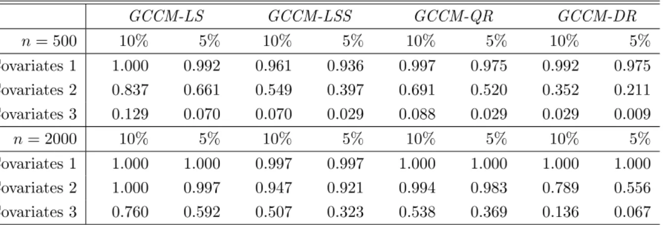
Table 2: Empirical Application: Empirical Rejection Frequencies of the Generalized Conditional Cramer van Mises (GCCM) Test for Correct Specification of various Conditional Distributional Models. GCCM-LS GCCM-LSS GCCM-QR GCCM-DR n= 500 10% 5% 10% 5% 10% 5% 10% 5% Covariates 1 1.000 0.992 0.961 0.936 0.997 0.975 0.992 0.975 Covariates 2 0.837 0.661 0.549 0.397 0.691 0.520 0.352 0.211 Covariates 3 0.129 0.070 0.070 0.029 0.088 0.029 0.029 0.009 n= 2000 10% 5% 10% 5% 10% 5% 10% 5% Covariates 1 1.000 1.000 0.997 0.997 1.000 1.000 1.000 1.000 Covariates 2 1.000 0.997 0.947 0.921 0.994 0.983 0.789 0.556 Covariates 3 0.760 0.592 0.507 0.323 0.538 0.369 0.136 0.067 GCCM denotes our Generalized Conditional Cramer van Mises test. Suffixes denote the spec-ification being tested: location shift (LS), location-scale shift (LSS), quantile regression (QR) or distributional regression (DR).

7. Empirical Application

In this section, we use our GCCM test to assess the validity of various commonly used models for the conditional distribution of wages given certain individual characteristics. As pointed out in the introduction, such models play an important role in the literature on decomposing counterfactual distributions (Fortin et al., 2011). There are doubts, however, that standard models like linear quantile regression are able to capture some important features of conditional wage distributions, such as e.g. the irregular behavior around the minimum wage. The results in this subsection shed some light on this important empirical issue.

We use a data set constructed from the 1988 wave of the Current Population Sur-vey (CPS), an extensive surSur-vey of US households. The same data is used in DiNardo, Fortin, and Lemieux (1996), to which we refer for details of its construction. It con-tains information on 74,661 males that were employed in the relevant period, including the hourly wage, years of education, years of potential labor market experience, and in-dicator variables for union coverage, race, marital status, part-time status, living in a Standard Metropolitan Statistical Area (SMSA), type of occupation (2 levels), and the industry in which the worker is employed (20 levels). As in the previous subsection, we consider the location shift model (LS), the location-scale sift model (LSS), the linear

quantile regression model (QR), and the distributional regression model (DR) using the normal CDF as a link function. We test the correct specification of each model with log hourly wage as the dependent variable, and the following three different subsets of the explanatory variables, respectively:

• Covariates 1: union coverage, education, experience.

• Covariates 2: all variables in Covariates 1, experience (squared), education inter-acted with experience, martial status, part-time status, race, SMSA.

• Covariates 3: all variables in Covariates 2, occupation, industry.

Given the large sample size, we would expect all specifications to be rejected by the data, since every statistical model is at best a reasonable approximation to the true data generating mechanism. However, this would not directly imply that such specifications result in misleading conclusions, as in large samples our GCCM test should be able to pick up deviations from the null hypothesis even if they are not of economically significant magnitude. On the other hand, we would have much more reason to be concerned if flexible models using many covariates would be rejected even in small samples. We therefore conduct a simulation experiment, where in each run we test the validity of various conditional distributional models using Covariates 1–3, respectively, for random subsamples of the data of sizen = 500 and n= 2000.

In Table 2, we report the empirical rejection probabilities from 1000 replications of the simulation experiment described above. We can see that using the information in Covariates 1 and Covariates 2 none of the four specifications we consider lead to an adequate fit of the conditional wage distribution. All empirical rejection rates are close to one for both sample sizes in case of Covariates 1. For Covariates 2, we observe rejection rates between about 22% and 66% at the nominal 5% level for n= 500, with the lowest rates coming from the DR model. For n = 2000, the QR specification (or one of its special cases) are rejected in almost all runs at the 5% level, while rejection rates for the DR model are somewhat lower at about 55%. For the most extensive set Covariates 3, rejection rates for all specifications are around or below the respective nominal level for n= 500. When moving to n= 2000, rejection rates for the QR specification rise to about

37% at the 5% nominal level. The LSS and LS specification are rejected at a similar or higher rate, respectively. On the other hand, rejection rates for the DR model remain around the respective nominal level in this case. Our simulation results in the previous subsection suggest that this last finding should not be due to a lack of power of our test under the DR specification. The class of distributional regression models might thus be more adequate to capture the particular features of conditional wage distributions, such as e.g. the nonlinearities close to the legal minimum wage level.

Remark 1. A particular feature of the CPS data is that the empirical distribution of hourly wages contains a number of mass points, since many workers are paid a “round” amount of dollars, or at least report it in the survey. Since the linear quantile regression model implies a strictly increasing conditional CDF, it is not able to reproduce such patterns. In order to check whether our high rejection rates are simply due to this issue, we repeated the above empirical exercise with the following modification: First, we computed the rank of each individual in the distribution of wages, breaking ties at random. Second, we replaced the observed wage by the quantile of a smoothed version of the empirical distribution of wages (obtained by linear interpolation of jump points) corresponding to the individual’s rank. That is, we were “spreading” the mass points evenly in order to obtain a “smooth” distribution of wages without ties. The results of our empirical exercise remained qualitatively unchanged using the modified data set, and are hence not reported for brevity. There are no theoretical issues related to mass points in the distribution of outcomes when using the class of distributional regression models, which was also confirmed in our simulation.

8. Conclusions

This paper provides a specification test for a general class of conditional distributional models indexed by function-valued parameters. Our method is straightforward to imple-ment and does not require the choice of smoothing parameters. We establish consistency of our testing procedure against fixed alternatives under general conditions, and study its local power properties. We illustrate the usefulness of our procedure via a simulation pro-cedure, highlighting its favorable practical properties compared to a competing approach.

In an application to real data, we show that our test is able to detect misspecification of standard linear quantile regression models for conditional distribution of wages in the US even in small samples, while a rich distributional regression model can typically not be rejected.

A. Appendix

A.1. Proofs of Theorems. In this subsection, we collect the proofs of our main the-orems. Some auxiliary results needed in the course of the proofs are given in Section A.2 of this Appendix.

Proof of Theorem 1. Recall the definition that

H0(y, x) = Z

t≤x

F(y|t, θ0)dG(t),

where under the assumptions of the theorem θ0 is well-defined under both the null and the alternative as the probability limit of the estimateθb_n. Also note that by construction H0 ≡ H under the null, and that P(H0(Y, X) 6= H(Y, X)) > 0 under the alternative. We also define the processes

ν(y, x) = √n(Hbn(y, x)−H(y, x)) and ν0(y, x) = √n(Hb_n0(y, x)−H0(y, x)),

and note that √

nRbn(y, x) = (ν(y, x)−ν0(y, x)) + √

n(H(y, x)−H0(y, x)).

To prove part i) of the theorem, we use the fact that under the null our test statistic can be rewritten as follows: Tn = Z (ν(y, x)−ν0(y, x))2dH(y, x) + Z (ν(y, x)−ν0(y, x))2d(Hb_n(y, x)−H(y, x)).

zero Gaussian process. Applying the Continuous Mapping Theorem and the Glivenko-Cantelli Theorem, we thus have that

Tn = Z

(_G1(y, x)−G2(y, x))2dH(y, x) +op(1),

as claimed. To show part ii), note that under a fixed alternative we have that

Tn = Z

(ν(y, x)−ν0(y, x) + √

n(H(y, x)−H0(y, x)))2dH(y, x) +op(1) =Op(n)

since H0 and H differ on a set with positive probability under the alternative. The test statistics becomes arbitrarily large with probability approaching 1 as n → ∞ in this case.

Proof of Theorem 2. To prove the result, we first define the empirical processesλ1(y, x) = √ n((Hb_n(y, x)− R F∗(y|t)_I{t ≤x}dG(t)) and λ2(θ, u) = √ n(Ψb_n(θ, u)−E_F∗(ψ(Z, θ, u))),

and denote the joint process by λ(y, x, θ, u) = (λ1(y, x), λ2(θ, u)). It then follows with Lemma 3 that

λ⇒_G1+δµ1,Ge1 +δeµ2

,

where µ1(y, x) = R(Q(y|t) − F∗(y|t))_I{t ≤ x}dG(t) and µ2_e (θ, u) = _EQ(ψ(Z, θ, u))−

EF∗(ψ(Z, θ, u)). Next, define the empirical processes ν∗(y, x) =

√

n(Hb_n(y, x)−H∗(y, x)) and ν₀∗(y, x) = √n(Hb_n0(y, x)−H∗(y, x)), with H∗(y, x) =

R

F∗(y|t)_I{t ≤ x}dG(t). Pro-ceeding in the same way as in the proof of Lemma 2, we find that

(ν, ν0)⇒(_G1+δµ1,G2+δµ2),

where µ2(y, x) =

R _˙

F(y|t)[h]_I{t ≤ x}dG(t) and h(u) = ∂θ0Ψ_F∗(θ_∗(u), u)−1Ψ_Q(θ_∗(u), u).

The statement of the Theorem then follows from the continuous mapping theorem, in the same way as in the proof of Theorem 1.

Proof of Theorem 3. To prove part i) let c(α) be the “true” critical value satisfying P(Tn > c(α)) = α +o(1). Then it follows from Lemma 4 that bcn(α) = c(α) +op(1). This implies that Tn and Te_n =T_n−(

distri-To prove part ii), note that by Lemma 4 the bootstrap critical value _bc(α) is bounded in probability under fixed alternatives. Hence for any > 0 there exists a sufficiently large constantM such thatP(_bcn(α)> M)< +o(1). Using elementary inequalities, we

also have that

P(Tn≤bcn(α)) = P(Tn≤bcn(α), Tn≤M) +P(Tn≤bcn(α), Tn > M) ≤P(Tn≤M) +P(bcn(α)> M).

From Theorem 1(ii), we know thatP(Tn≤M) =o(1), and thusP(Tn≤bcn(α))< +o(1), which implies the statement of the theorem since can be chosen arbitrarily small.

To show part iii), define c(α) as in the proof of part i), i.e. the α-quantile of the limiting distribution of the test statistic Tn under the null hypothesis. Using Anderson’s

Lemma, we find that

P Z (_G1(y, x)−G2(y, x) +µ(y, x))2dH(y, x)> c(α) ≥P Z (_G1(y, x)−G2(y, x))2dH(y, x)> c(α) =α,

because the Gaussian process_G1−G2 has mean zero (see also Andrews (1997, p. 1114)). Under a local alternative, we therefore have thatP(Tn> c(α))≥α+o(1). Furthermore,

we have already shown in part i) that P(Tn > bcn(α)) = P(Tn > c(α)) +o(1) under the null hypothesis. By using contiguity arguments, this can also shown to be true under the local alternative, see e.g. the proof of Corollary 2.1 in Bickel and Ren (2001).

Proof of Theorem 4–6. This follows by straightforward applications of results in Cher-nozhukov et al. (2009, Appendix F).

A.2. Auxiliary Results. In this subsection, we collect a number of auxiliary results used in the proofs of our main results above.

Lemma 1. Define the empirical processesν(y, x) =√n(Hbn(y, x)−H(y, x))andw(θ, u) =

√

n(Ψb_n(θ, u)−Ψ(θ, u)). Then, under either the null hypothesis or a fixed alternative, and

tight bivariate mean zero Gaussian process. Moreover, the bootstrap procedure in Section 2.3 consistently estimates the law of Ge.

Proof. This lemma is a minor generalization of Lemma 13 in Chernozhukov et al. (2009), and can thus be proven in the same way.

Lemma 2. Let either the null hypothesis or a fixed alternative, and Assumptions 1-6 be true. Define the empirical processes ν(y, x) = √n(Hb_n(y, x)−H(y, x)) and ν₀(y, x) = √

n(Hb_n0(y, x)−H0(y, x)). Then it holds that(ν, ν0)⇒Ginl∞(Z×Z), whereG= (G1,G2)

is a tight bivariate mean zero Gaussian process.

Proof. Under either the null hypothesis or a fixed alternative, it follows from our Lemma 1 and Lemma 11 in Chernozhukov et al. (2009) that

√ n   b Hn(·,·)−H(·,·) b θn(·)−θ0(·)  ⇒   G1(·,·) −Ψ˙−_θ01_(·),·[Ge₂(θ₀(·),·)]  

in`∞(Z)×`∞(T). Next, it follows from Assumption 5 that √

n(Fb_n(y|x)−F(y|x))⇒ −F˙(y|x, θ₀)[ ˙Ψ−_θ01_(·),·[Ge₂(θ₀(·),·)]] =:G∗₂(y, x).

The statement of the Lemma then follows directly from Hadamard differentiability of the mapping (A, B)7→R

A(·)_I{t≤ ·}dB(t), and the Functional Delta Method. In particular, for the second component_G2 of the joint limiting process we have that

G2(y, x) = Z

F(y|t)_I{t≤x}d_G1(∞, t) + Z

G∗2(y, t)I{t≤x}dG(t),

which follows from the form of the Hadamard differential of the mapping (A, B) 7→ R

A(·)_I{t≤ ·}dB(t).

Lemma 3. Suppose the data are distributed according to a local alternative Qn

sat-isfying Assumption 7. Define the processes vn(y, x) =

√ n(Hb_n(y, x) − H_n(y, x)) and wn(θ, u) = √ n(Ψbn(θ, u) − Ψn(θ, u)), where Hn(y, x) = R Qn(y|t)I{t ≤ x}dG(t) and Ψn(θ, u) = EQn(ψ(Z, θ, u)). Then it holds (vn, wn) ⇒ Ge in l ∞_{(Z ×Θ×T), where the}

Proof. This follows by an application of Lemma 2.8.7 in Van der Vaart and Wellner (1996), using the fact that by Assumption 4,Qnis the linear combination of two measures

under which the function class G is Donsker with a square integrable envelope.

Lemma 4. Define the bootstrap empirical processes νb(y, x) =

√

n(Hb_b,n(y, x)−Hb_n0(y, x))

and νb,0(y, x) = √

n(Hb_b,n0 (y, x)−Hb_n0(y, x)). Then it holds under either the null hypothesis

or a fixed alternative that (νb, νb,0)⇒Gb, where Gb = (Gb1,Gb2) is a tight bivariate mean

zero Gaussian process whose distribution coincides with that of the process _Gin Lemma 1 under the null hypothesis.

Proof. This follows from Lemma 1 and the Functional Delta Method for the bootstrap (Van der Vaart and Wellner, 1996, Theorem 3.9.11)

B. Sufficient Condition for Contiguity.

In this section, we show that the condition given in (3.2) is sufficient for contiguity. Our argument is analogous to the one given in Andrews (1997), and stated here only for completeness. For and distribution function H, let PH be the probability mea-sure induced by H. By definition, PHn _{is contiguous to P}H∗ _{if P}H∗_(A

n) → 0 implies PHn_(A

n)→ 0 for every sequence of measurable sets An. By an application of Le Cam’s

First Lemma (Van der Vaart, 2000, Theorem 6.4) this is the case if dPHn_/dPH∗

con-verges in distribution to a random variable V with _E(V) = 1 underPH∗. We show that log(dPHn_/dPH∗₎ →d _N(−_σ2_{/2, σ}2_{) for some value σ}2 _{> 0, which directly implies that}

the aforementioned condition is fulfilled (see also Example 6.5 in Van der Vaart (2000)). Writingan=δ/

√

n, it holds by the definition of dPHn _{and dP}H∗ _that

dPHn dPH∗ = Qn i=1((1−an)f ∗ (Yi|Xi)g(Xi) +anq(Yi|Xi)g(Xi)) Qn i=1f∗(Yi|Xi)g(Xi) ,

and we thus have that log dPHn dPH∗ = n X i=1 log (1−an)f∗(Yi|Xi)g(Xi) +anq(Yi|Xi)g(Xi) f∗_(Y i|Xi)g(Xi) = n X i=1 log 1 +an q(Yi|Xi)−f∗(Yi|Xi) f∗_(Y i|Xi) = n X i=1 log(1 +Zi), where Zi =an q(Yi|Xi)−f∗(Yi|Xi) f∗_(Y i|Xi) .

A Taylor expansion of log(1 +Zi) around 1 yields

log dPHn dPH∗ = n X i=1 Zi− 1 2Z 2 i + 1 6Z 3 i 2 (1 +ξi)3

for some ξi ∈ [−Zi, Zi], as log(1) = 0.Next, we show that by the central limit theorem

Pn

i=1Zi converges in distribution to a normally distributed random variable, that by

the law of large numbers Pn

i=1Z

2

i converges almost surely to a constant, and that the

remaining summand Z_n∗ := n X i=1 1 6Z 3 i 2 (1 +ξi)3 converges to 0 in probability.

First consider the expectation of the random variableZe_i =δ

q(Yi|Xi)−f∗(Yi|Xi) f∗_(Y i|Xi) underP: E(Ze_i) =δ Z Z q(y|x)−f∗(y|x) f∗_(y|x) f ∗ (y|x)dµ(y)dG(x) =δ Z Z (q(y|x)−f∗(y|x))dµ(y)dG(x) =δ Z Z q(y|x)dµ(y)dG(x)−δ Z Z f∗(y|x)dµ(y)dG(x) = δ−δ= 0.

Furthermore, note that with (3.2) we have that

E(|Z|p) =E q(Yi|Xi) −1 p <∞

for all values of p. Since Pn i=1Zi = 1 √ n Pn

i=1Zei, we can directly apply the standard

central limit theorem for i.i.d. random variables and get

n X i=1 Zi d →N0,_E(Ze_i)2 . Moreover, we have Pn i=1Z 2 i = n1 Pn i=1(Ze_i)2. As E (Ze_i)2

<∞, the usual strong law of

large numbers yields

n X i=1 Z_i2 →a.s.E (Zei)2 .

To show convergence of the remaining summand to 0, we apply Markov’s inequality to Z_n∗. For any >0, we have

E(|Zn∗|) ≤ 1 6 1 √ nE(|Ze 3 i|)E 2 |(1 +ξi)3| . (B.1)

Since we have ξi ∈[−Zi, Zi], and since (3.3) implies that

|Zi|= 1 √ nδ q(Yi|Xi) f∗_(Y i|Xi) −1 ≤C1/ √ n

for a constant C1, we obtain the bound |ξi| < 1 for sufficiently large n. Therefore, the

expression on the right-hand side of (B.1) is bounded, and we find that for arbitrary >0, sufficiently large n and a constant C2 it holds that

P(|Zn∗|> )≤ E(|Zn∗|) ≤ C2 √ n,

and thus Z_n∗ →p 0, as claimed. Taken together, we now thus show that

log dPHn dPH∗ d →N −1 2E (Zei)2 ,_E (Zei)2 ,

References

Albrecht, J., A. Van Vuuren, and S. Vroman (2009): “Counterfactual

distribu-tions with sample selection adjustments: Econometric theory and an application to the Netherlands,”Labour Economics, 16, 383–396.

Andrews, D. (1997): “A conditional Kolmogorov test,”Econometrica, 65, 1097–1128.

Bickel, P. and J.-J. Ren (2001): “The bootstrap in hypothesis testings,” Lecture

Notes-Monograph Series, 36, 91–112.

Bierens, H.(1990): “A consistent conditional moment test of functional form,”

Econo-metrica, 1443–1458.

Bierens, H. and D. Ginther(2001): “Integrated conditional moment testing of

quan-tile regression models,” Empirical Economics, 26, 307–324.

Bierens, H. and W. Ploberger(1997): “Asymptotic theory of integrated conditional

moment tests,”Econometrica, 65, 1129–1151.

Billingsley, P.(1995): Probability and measure, Wiley.

Chernozhukov, V., I. Fernandez-Val, and B. Melly(2009): “Inference on

Coun-terfactual Distributions,”Working Paper.

Chernozhukov, V. and C. Hansen (2005): “An IV model of quantile treatment

effects,”Econometrica, 73, 245–261.

DiNardo, J., N. Fortin, and T. Lemieux (1996): “Labor market institutions and

the distribution of wages, 1973-1992: A semiparametric approach,” Econometrica, 64, 1001–1044.

Escanciano, J. and C. Goh (2010): “Specification Analysis of Structural Quantile

Regression Models,”Working Papers.

Escanciano, J. and C. Velasco (2010): “Specification tests of parametric dynamic

Foresi, S. and F. Peracchi(1995): “The Conditional Distribution of Excess Returns:

An Empirical Analysis.”Journal of the American Statistical Association, 90, 451–466.

Fortin, N., T. Lemieux, and S. Firpo (2011): “Decomposition Methods in

Eco-nomics,” Handbook of Labor Economics, 4, 1–102.

Galvao, A., K. Kato, G. Montes-Rojas, and J. Olmo (2011): “Testing linearity

against threshold effects: uniform inference in quantile regression,”Working Paper.

Harvey, A.(1976): “Estimating regression models with multiplicative

heteroscedastic-ity,”Econometrica, 461–465.

He, X. and L. Zhu (2003): “A lack-of-fit test for quantile regression,” Journal of the

American Statistical Association, 98, 1013–1022.

Horowitz, J. and V. Spokoiny (2001): “An Adaptive, Rate-Optimal Test of a

Para-metric Mean-Regression Model Against a NonparaPara-metric Alternative,” Econometrica, 69, 599–631.

——— (2002): “An adaptive, rate-optimal test of linearity for median regression models,”

Journal of the American Statistical Association, 97, 822–835.

H¨ardle, W. and E. Mammen (1993): “Comparing nonparametric versus parametric

regression fits,” The Annals of Statistics, 21, 1926–1947.

Koenker, R. (2005): Quantile regression, Cambridge University Press.

——— (2010): “On Distributional vs. Quantile Regression,” Working Paper.

Koenker, R. and G. Bassett(1978): “Regression quantiles,” Econometrica, 46, 33–

50.

Koenker, R. and J. Machado(1999): “Goodness of fit and related inference processes

for quantile regression,”Journal of the American Statistical Association, 94, 1296–1310.

Koenker, R. and Z. Xiao (2002): “Inference on the quantile regression process,”