Resampling Methods For Markov Processes With No Mixing Constraints

(1)

RESAMPLING METHODS FOR MARKOV PROCESSES

WITH NO MIXING CONSTRAINTS

A THESIS SUBMITTED TO THE GRADUATE DIVISION OF THE UNIVERSITY OF HAWAI‘I AT M ¯ANOA IN PARTIAL FULFILLMENT

OF THE REQUIREMENTS FOR THE DEGREE OF

MASTER OF SCIENCE IN ELECTRICAL ENGINEERING DECEMBER 2017 By Kevin Oshiro Thesis Committee:

Narayana Santhanam, Chairperson James Yee

(2)

Acknowledgements

First, I would like to thank my adviser Dr. Narayana Santhanam for his support and guidance. He has provided me with valuable lessons on many occasions and I am grateful to have had the opportunity to learn from him. I would also like to thank my committee members Dr. James Yee and Dr. June Zhang for their feedback on my research and for their advice in general. Furthermore, I would like to express my gratitude to fellow graduate students Maryam and Changlong for their occasional assistance and useful discussions regarding research and classes. I am also grateful to my friends for their encouragement and support in pursuing my academic goals. Finally, I would like to thank my parents for their love, support, and patience. It is because of them that I have been able to accomplish all that I have done.

(3)

Abstract

Jackknife and bootstrap are resampling procedures that can be used to reduce the bias or estimate the variance of a statistic. These methods are useful because they perform well and are simple to implement, but an important assumption for their good performance is that of i.i.d. sampling. Previous analysis of these techniques for processes with memory generally require constraints on the memory or the mixing.

In this work we adapt the jackknife and bootstrap procedures to estimate the variance of conditional probability estimates when we have unbounded memory and make no assumptions on the mixing of the process. We only require that the process satisfies a continuity condition, which says that the incremental value of a bit in the past diminishes with increasing distance. We then analyze the procedures to provide bounds on the bias of the estimates.

(4)

List of Tables

3.1 Empirical frequencies and stationary probabilities of original process for Example 6. 16 3.2 Empirical frequencies and stationary probabilities of aggregate process for Example 6. 16 3.3 Empirical and theoretical stationary probabilities for select states of process (3.4) . . 22 3.4 Empirical and theoretical transition probabilities for select states of process (3.4) . . 22 3.5 Empirical and theoretical stationary and transition probabilities for select states of

(7)

List of Figures

2.1 (2.1a) Context tree for the Markov process from Example 4, where the leaves are the probability of 1 given the context. (2.1b) Corresponding state transition diagram with transition and stationary probabilities. . . 11 2.2 (2.2a) Context tree for the aggregated process from Example 4. (2.2b) Corresponding

state transition diagram with transition and stationary probabilities. . . 11 3.1 (3.1a) States and transition probabilities for Markov process from Example 5. (3.1b)

Aggregated process withk= 1. . . 14 3.2 (3.2a) States and transition probabilities for Markov process from Example 6. (3.2b)

Aggregated process with k= 1. (3.2c) State transition diagram for Markov process from Example 6. (3.2d) Aggregated process withk= 1. . . 15 3.3 State transition diagram for Markov process from Example 7. . . 17 3.4 State transition diagram for Markov process from Example 9. . . 18 3.5 State transition diagram of base transition probabilities for slow mixing process (3.4) 21

(8)

Chapter 1

Introduction

Suppose we have a finite number of samples drawn from an unknown distribution, and using these samples we estimate some parameter of that distribution. One important question to ask is whether the estimate is good or not. In other words, how close do we expect it to be to the true value and if we were to obtain another sample and estimate again, how much would we expect our answer to vary? Of course, we can’t provide answers without knowing the true distribution, but what we can do is use the data to estimate these values. For this we can use resampling procedures such as jackknife or bootstrap. These techniques are favorable because they are easy to understand, straight foward to implement, and require few assumptions.

Jackknife allows one to reduce the bias or estimate the variance of a sample via recalculated statistics, obtained by sequentially omitting data points. Bootstrap is used to estimate the prop-erties of an estimator by drawing samples from the empirical distribution given by the sample. Cross-validation also falls into the category of resampling procedures, but it is used to estimate of the error associated with a predictive model built on data by systematically rotating different subsets of the data between training and validation.

One assumption which is essential for obtaining good results is that of independent sampling. It is easy to see that ignoring dependencies between the samples can give unfavorable results. Much work has been done to adapt these resampling procedures to general Markov and stationary ergodic setups. One group of results, [6], [7], [8], [9], [10], [11], and [12], considers grouping the samples into blocks. The jackknife procedures then operates by removing the blocks in some systematic manner,

(9)

while the bootstrap samples from the set of blocks. Another line of research, [13], [14], [15], [16], considers estimating the transition probabilities of the source and then generating new samples using the estimated source. However, these approaches generally require some sort of assumption on the mixing of the process, i.e., how quickly the empirical frequencies in the sample reflect the stationary probabilities of the source.

In this work we make no assumptions on the mixing of the process or the length of the memory. With no assumptions the problem is ill-posed, as Markov souces can have long enough memory and sufficiently slow mixing such that they are indistinguishable from an i.i.d. source for any sample size. Therefore we adopt a continuity condition, as in [1], which says that bits that are farther apart, conditioned on all bits between, have less information about each other. In other words, our condition acts as a soft memory constraint and does not at all constrain the mixing.

Given this setup, we apply the jackknife procedure to estimate the variance of the empirical transition probabilities and give a bound on the bias of the estimate. We also apply the bootstrap procedure for the same estimates and give a bound on the bias of the bootstrap estimate. Addition-ally, we will see that some interesting phenomena arise in the slow mixing regime; e.g., estimates for longer contexts can sometimes be better than estimates of their suffixes, despite having less data.

Motivation

To motivate the problem of estimating parameters of slow mixing Markov processes, we consider the following example. Suppose we have a hypothetical user browsing the internet for political news. Starting at one news site, the user follows one of the available hyperlinks to another site, then follows a link from that site, and so on. As many political news sites tend to be biased more liberal or conservative, they likely link mostly to other pages with a similar persuasion. Additionally, the beliefs held by the user influence which links are chosen. So the user will likely be confined to a certain subset of webpages and will obtain news only from sites with a particular set of opinions.

We can view this browsing of political webpages as a random walk on a graph, which lends itself to representation as a Markov process. Each webpage can be represented by a symbol from a finite alphabet, depending on the topic of interest. For example, we can have a 1 if the webpage

(10)

contains some number of keywords and a 0 otherwise. The transition probabilities of the process are dependent on the opinions of a particular user. Also note that we can reasonably assume that the more browser history we have, the less the additional information provided by obtaining another page of history.

Suppose we wish to quantify the polarization of opinions or information on a topic. More polarized user opinions equate to a slower mixing process. Therefore, to describe the polarization, we must obtain the transition and stationary probabilities of the process.

Given some user’s browser history, we are interested in the probability the user will click on certain links. We do not know the memory of the process, i.e., how many past pages affect the click probabilities. Therefore, what we can do is to pick a context length and make transition probability estimates given contexts of that length. As the process is slow mixing, it is likely we will only be able to obtain estimates for some of the browsing contexts.

(11)

Chapter 2

Background

In this section we will first discuss the original jackknife and bootstrap procedures for i.i.d. samples. We also briefly mention cross validation. Then we will describe Markov processes. Finally, we will examine some of the prior work that has been conducted on applying resampling procedures when samples are not i.i.d.

2.1

Jackknife

2.1.1 The Bias Estimate

Consider i.i.d. samplesX1, X2, . . . , Xngenerated from an unknown sourcepand an estimate ˆθ(X1n)

of θ, some real valued parameter of the source. The bias of an estimator,

Bias =E[ˆθ(X₁n)−θ],

is one measure of how good the estimator is. In words, the bias tells us the difference between the expected value of the estimate and the true value of the parameter.

Without knowing the distribution from which the samples were generated, the actual bias cannot be calculated. However, the jackknife procedure [2], which was introduced by Quenouille, can be used to estimate the bias. The procedure operates by sequentially removing samples and

(12)

applying the estimator to obtain the recomputed statistics,

ˆ

θi = ˆθ(X1, . . . Xi−1, Xi+1, . . . , Xn).

Then the bias estimate is

d

BiasJack= (n−1)(ˆθ(·)−θˆ), (2.1)

where ˆθ(·)= n1

Pn

i=1θˆi is the average of the recomputed statistics. For the bias corrected estimate we have

˜

θ= ˆθ−Biasd_Jack=nθˆ−(n−1)ˆθ₍_·₎. (2.2)

The estimate (2.2) is not necessarily unbiased, as Biasd_Jack is only an estimate of the true bias of

ˆ

θ. In general, the correction reduces the bias from O(_n1) toO(_n12). If the estimator is a quadratic

functional, i.e., it can be written in the form

ˆ θ=µ(n)+ 1 n n X i=1 α(n)(xi) + 1 n2 X 1≤i1≤i2≤n β(xi1, xi2), (2.3)

thenBiasd_Jack is unbiased in estimating the true bias of the estimator [2].

Examples 1 and 2, borrowed from [2], demonstrate the jackknife procedure performed on some common estimates.

Example 1 (The Variance) LetX1, X2, . . . , Xnbe i.i.d. samples drawn from some distribution. The sample mean is ¯X = _n1Pn

i=1Xi and the sample variance is ˆθ = _n1Pin=1(Xi −X¯)2. Then ˆ θi = _n−11 P j6=i(Xj−X¯i)2 and ˆθ(·) = n1 P iθˆi, where ¯Xi = _n−11 P j6=iXj. Applying (2.1) and (2.2) gives bias estimate

(13)

d BiasJack = (n−1)(ˆθ(·)−θˆ) = (n−1) 1 n X i 1 n−1 X j6=i (Xj−X¯i)2 − 1 n X i (Xi−X¯)2 = n−1 n X i X_i2− 2 n X i 1 n−1 X j6=i Xj X j6=i Xj +n−1 n X i 1 n−1 X j6=i Xj 2 − n−1 n X i X_i2+2(n−1) n 1 n X i Xi X i Xi− n−1 n X i 1 n X j Xj 2 =− 1 n(n−1) X i X j6=i Xj 2 + n−1 n2 X i Xi 2 = 1 n2₍_n₋₁₎ X i X j XiXj− 1 n(n−1) X i X_i2 =− 1 n(n−1) X i (Xi−X¯)2,

and the bias corrected estimate is

˜ θ= 1 n−1 n X i=1 (Xi−X¯)2,

which is the well known unbiased estimate of the variance.

2.1.2 The Variance Estimate

Another measure of the quality of an estimator is its variance,

Var =E[(ˆθ−Eθˆ)2].

Tukey expanded on the jackknife procedure, using the recomputed statistics to obtain an estimate of the variance of the estimator with

d VarJack= n−1 n n X i=1 (ˆθi−θˆ(·))2. (2.4)

Example 2 (The Expectation) Let X1, X2, . . . , Xn be as in Example 1. Here the statistic of interest is ˆθ= ¯X = 1_nPn i=1Xi. Then ˆθi = nθˆ−Xi n−1 , ˆθ(·) = ˆθ, and ˆθi−θˆ(·) = ¯ X−Xi n−1 . Therefore, from

(14)

(2.4), d VarJack= Pn i=1(Xi−X¯)2 n(n−1) .

The variance estimate can be thought of as an estimate of the variance of the statistic on a sample of sizen−1 and then a scaling to sample size n. Let Varn−1 be the variance of the statistic

on a sample of size n−1, and let

g Var = n X i=1 (ˆθi−θˆ(·))2

be the estimate of Varn−1. Then

d

VarJack=

n−1

n Varg.

The main result from [3] is

E[Var]g ≥Var_n−1,

that the variance estimate for sample sizen−1 is biased upwards in general. More specifically, ifθ

is a linear functional, i.e., it can be expressed as ˆθ=µ+_n1 P

iα(Xi), then E[gVar] = Var_n−1. This

is shown via the ANOVA decomposition which splits θas

θ=µ+X i Ai(Xi) +X i≤i0 Bii0(X_i, X_i0) + X i≤i0_≤_i00 Ci,i0_,i00(X_i, X_i0, X_i00) +· · ·+H(X₁, X₂, . . . Xn),

where µ=E[θ] is called the grand mean,Ai(xi) =E[θ|Xi =xi]−µ theith main effect,Bxi,xi0 = E[θ|Xi =xi, Xi0 =x_i0]−E[θ|X_i =xi]−E[θ|X_i0 =x_i0] +µ theii0th second order interaction, etc. The Ai’s,Bii0’s, etc., have mean zero and are uncorrelated. Then the variance can be written as

Var(θ(X₁n)) = σ 2 α n + n−1 1 _σ2 β 2n3 + n−1 2 _σ2 γ 3n5 +· · ·+ σ2 η n2n,

where σ2_α = Var(nA(Xi)), σ_β2 = Var(n2B(Xi, Xi0)), σ_γ2 = Var(n3C(X_i, X_i0, X_i00)), etc. A similar

form can be obtained for E[Var], and in the bias theg _n1 term is cancelled out, while the result is

(15)

2.2

Bootstrap

The bootstrap, introduced by Efron in [4], is another popular resampling procedure. Again consider samplesX1, X2, . . . , Xn drawn i.i.d. from some unknown distribution p and an estimate ˆθ(X1n) of

parameter θ. Now suppose we wish to estmate the variance of ˆθ(X₁n). Let ˆp be the empirical

distribution given by X₁n. Then the bootstrap estimate of the variance is obtained by simply

evaluating the variance of the estimator on ˆp. Depending on the estimator, it may not be possible to explicitly calculate the variance, and so the Monte Carlo algorithm is used. To do this, begin by sampling (with replacement) from the empirical distribution to obtain i.i.d. X₁∗b, X₂∗b, . . . , X_n∗b.

Calculate the estimate on the bootstrap sample, ˆθ∗b _{= ˆ}_θ₍_X∗b

1 , X2∗b, . . . , Xn∗b). Repeat the process to obtain B bootstrap replications ˆθ∗1,θˆ∗2, . . . ,θˆ∗B. The bootstrapped estimate of the variance is

then, d VarBoot = PB b=1(ˆθ ∗b₋_θˆ∗•₎2 B−1 (2.5) where ˆθ∗•= _B1 PB b=1θˆ ∗b_.

The following example adapted from [2], illustrates the bootstrap procedure for the variance of the average.

Example 3 (The Average) LetX1, X2, . . . , Xn be i.i.d. samples from a distribution with mean

µ and variance σ2, and let ˆθ(X₁n) = ¯X = _n1 Pn

i=1Xi. In this case we know that Var( ¯X) =

σ2 n. Therefore the bootstrap variance estimate isVard_Boot= 1

n2

Pn

i=1(Xi−X¯)2.

The procedure can be applied to obtain estimates of other functions of θas well. For example, to estimate P r(θ≤ c) for some constant c, we have P r(ˆθ∗ ≤c) = _B1 PB

b=1I{θˆ

∗b _≤ _c_}_{, where}_I _is the indicator function.

For the bias, the bootstrap estimate is

d BiasBoot= 1 B B X b=1 ˆ θ∗b−θˆ= ˆθ∗•−θ.ˆ (2.6)

In [2] it is shown that if ˆθ is a quadratic functional, see (2.3), then

d

BiasBoot =

n−1

(16)

Variations of the bootstrap method include drawing the bootstrap samples from a parametric model, e.g., a Gaussian distribution with the sample mean and variance, or using a smoothed empirical distribution obtained by convolving with a scaled normal distribution.

2.3

Cross-Validation

Cross-validation is another well known technique which falls into the category of resampling proce-dures. See [5]. In contrast to bootstrap and jackknife, it is generally used to estimate the error of a model built on data. Typically the data is partitioned into two sets, training and validation. The first is used to train the model and the second is used to test it, giving some error. This is then repeated multiple times by taking a different partition in some systematic manner and an average error can be obtained. For example, k-fold cross-validation involves partitioning the data into k

sets, training on k−1 of the sets, and validating on the last set, repeating k times for each of the possibilities. In leave-one-out cross-validation, the model is training on all but one of the data points, then tested on the omitted one. The processes is then repeated for each of the data points.

2.4

Markov Processes

A Markov processpT with finite alphabetAis defined by a suffix-free set of statesT ⊂A∗=∪k≥0Ak

and a set of transition probabilities p(T) = {p(a|s) > 0 : a ∈ A,s ∈ T }. The set T can be represented as a fullA-ary tree where the leaves correspond to the states. The process has memory

D = max{|s|:s ∈ T }, also equal to the depth of the tree. Here we will consider binary Markov processes, soA={0,1}.

If a Markov process is aperiodic, irreducible1, and has finite state space, then it has a unique

stationary distributionπ satisfying

π =πP,

where P is the transition matrix for the Markov chain; i.e., Pij is the probability of moving from stateito statej in one step.

1

The processes considered here are aperiodic since any states∈ T can be reached in either|s|or|s|+ 1 steps and irreducible sincep(a|s)>0 for alla∈ Aands∈ T.

(17)

The following provides an example of a Markov process along with the context tree and state transition diagrams. The example also serves to intuitively illustrate some of the complications associated with estimating parameters of Markov processes.

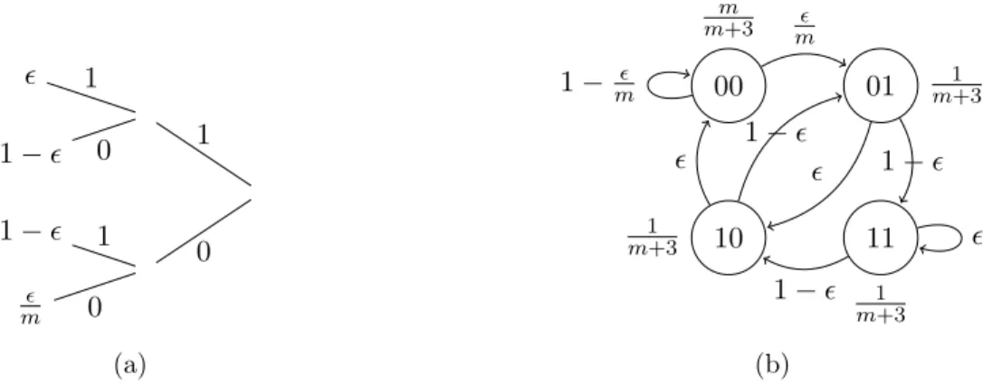
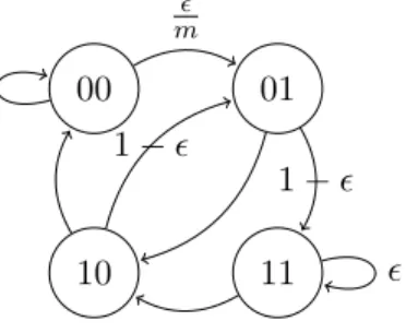
Example 4 Let A = {0,1} and T = {00,01,10,11}, with p(1|00) = _m, p(1|01) = 1 −,

p(1|10) = 1−, and p(1|11) = . For m > > 0, the model pT represents a stationary ergodic

Markov process with stationary distributionπ(00) = _mm₊₃, and π(01) =π(10) =π(11) = _m1₊₃.

The leaves of the tree in Figure 2.1a show the conditional probability of 1 given the corresponding context. Figure 2.1b displays the state transition diagram along with the transition and stationary probabilities.

First we use this example to introduce the context tree and state transition diagrams. Suppose we had past samples X−3X−2X−1X0= 1001. The state of the process is the suffix of the past bits

that is in T, which in this case is 01. Then p(X1 = 1|X−03) =p(X1 = 1|X−01) = 1−, since only

the past at most D= 2 bits matter. Now suppose X1 = 1. Then X−13 = 10011, the current state

is 11, and the next bit is a 1 with probability . Now suppose X2 = 0. Then X−23 = 100110, the

state becomes 10, and so on.

Next we try to provide some intuition for the problems we face while making estimates with samples from a Markov process. Let 1

n, where n is the sample size, and let m be large. If our process starts in state 01, 11, or 10, then with high probability our sample will look like

. . .011011011011. . .. It is unlikely we will observe the state 00, since p(0|10) is very small, even though 00 can have stationary probability which is arbitrarily close to 1. Additionally, we are not able to estimate the transition probability for 00 if it doesn’t occur.

Suppose that we did not know the memory of the process or the set of states. Then we may reasonably choose to estimate p(1|1) and p(1|0). Based on our sample, we would guess 1₂ and 1, respectively. Using the aggregate model, shown in Figure 2.2, which is discussed in the following chapter, the actual probabilities can be calculated as p(1|1) = 1₂ and p(1|0) = _m1₊₁. We may have gotten p(1|1) correct, but our estimate for p(1|0) is about as far off as can be.

(18)

1 1− 0 1 1− ₁ m 0 0 (a) 00 m m+3 01 _m1₊₃ 10 1 m+3 11 1 m+3 m 1− m 1− 1 − 1− (b)

Figure 2.1: (2.1a) Context tree for the Markov process from Example 4, where the leaves are the probability of 1 given the context. (2.1b) Corresponding state transition diagram with transition and stationary probabilities.

1 2 ₁ 1 m+1 0 (a) 0 m+1 m+3 1 2 m+3 m m+1 1 m+1 1 2 1 2 (b)

Figure 2.2: (2.2a) Context tree for the aggregated process from Example 4. (2.2b) Corresponding state transition diagram with transition and stationary probabilities.

2.5

Prior Work on Resampling Methods for Markov Processes

One assumption which is essential in obtaining good results for the classical jackknife and bootstrap is that the samples are i.i.d. It is easy to see that the procedures produce poor results if the dependencies in the data are ignored. Much work has gone into adapting the jackknife and bootstrap for various situations in which the data is not i.i.d. Some of this work has focused solely on either the jackknife or the bootstrap, whle others have techniques applicable to both.

The first category of results involves grouping samples in some systematic manner. In [6] a natural extension of the jackknife is introduced, where the length-n data is partitioned into b

nonoverlapping blocks of length l = n_b, and these blocks are removed one by one to obtain the recalculated statistics. It is shown that the estimator is consistent under certain conditions and also how to obtain the optimal choice for the block length. For the case that the data is from a general stationary sequence with weak dependence, [7] proposed a variation with overlapping blocks,

(19)

where the jackknife procedure omits one block at a time and the bootstrap procedure independently samples the n−l+ 1 blocks. Here the jackknife estimates are shown to be consistent if the block length l tends to infinity at an appropriate rate. In [8], the same overlapping block procedure was independently proposed for samples which are from a stationary m-dependent2 process. A

further extension, the blocks of blocks scheme, was proposed in [9], [10], [11]. Their aim was to allow for estimators involving parameters of the entire joint distribution, e.g., the spectral density. The procedure in [12] takes a slightly different approach to selecting blocks of samples. They randomly select an initial sample, then with probabilityppick the next sequential sample and with probability 1−p randomly select any of the n samples. They then show the pseudo time series with geometrically distributed block lengths generated from this procedure is also stationary.

Another category of results involve estimating the transition density from the samples in order to generate more data. The Markov conditional bootstrap is introduced in [13], which estimates the transition density nonparametrically and then samples from the estimated density. It is also shown that this improves upon the block bootstrap, albeit under stronger conditions. Implicit estimation of the one step transition distribution is performed in [14], where samples from a stationary Markov process are sampled locally in order to reproduce the dependence properties of the process. The sampling procedure selects the next sample randomly from the set of valuesXs+1 such that|Xt−

Xs| ≤ b, where Xt is the current sample. [15] imposes conditional moment restrictions on the process and performs a weighted empirical estimate of the one step conditional distribution. In [16], the source is approximated by a family of parametric models, one of which is then chosen based on the data.

All of these results generally depend upon implicit or explicit mixing assumptions to obtain good estimates.

2_{A process}_{_X

i},i= 1, . . . , nism-dependent if for any pair of eventsAandB, whereAdepends on{X1, . . . , Xk}

(20)

Chapter 3

Slow Mixing Setup

In this chapter we detail some of the potential problems encountered when making estimates with unbounded memory and no assumptions on the mixing. Next we describe our continuity condition, which allows us to be able to make reasonable estimates. Then we discuss some results from [1] involving the estimation of transition probabilities from processes that satisfy a continuity condition. We also show some simulation results of estimates made in a slow mixing process to illustrate some interesting artifacts.

3.1

Aggregated Model

Suppose we have samplesX1, X2, . . . , Xn from a binary, ergodic, aperiodic Markov processpT. We

can represent the state space of the process with the leaves of a full binary treeT, which we assume has finite depth. Using only the samples, we wish to estimate parameters of pT.

As we have no knowledge of the actual memory or set of states, we approximate the source with an aggregated modelpT˜, which has state space ˜T ={0,1}kn. We letkn scale logarithmically with

n for consistency, as in [17]. Now we can make estimates for parameters of the aggregate source. Lets∈ T be a state of the original process and letw∈T˜ be a state of the aggregated process. To denote thatwis a suffix ofs, we writew≺s.

(21)

Note that, in general, w is not an a state of pT, since we have no knowledge of the memory.

Then for a∈ {0,1} we have

p(w) = X s0_∈T_,_w_≺_s0 p(s0) and p(a|w) = 1 p(w) X s∈T,w≺s p(s)p(a|s) for the aggregated stationary and conditional probabilities, respectively.

Here we give an example of calculating the probabilities for an aggregated process.

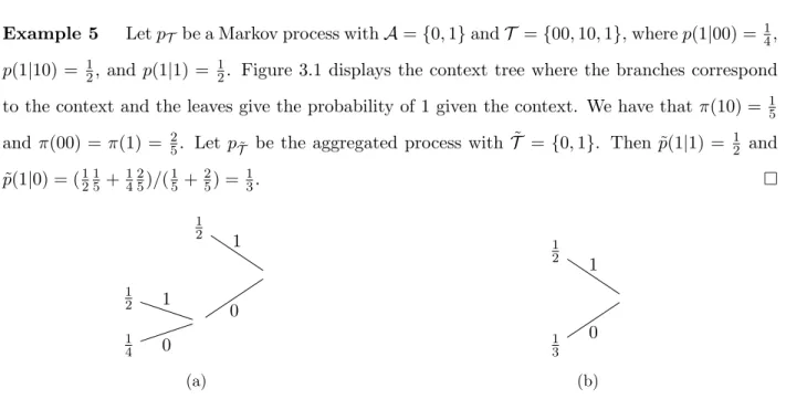
Example 5 LetpT be a Markov process withA={0,1}andT ={00,10,1}, wherep(1|00) = 1₄, p(1|10) = 1₂, and p(1|1) = 1₂. Figure 3.1 displays the context tree where the branches correspond to the context and the leaves give the probability of 1 given the context. We have that π(10) = 1₅

and π(00) = π(1) = 2₅. Let pT˜ be the aggregated process with ˜T = {0,1}. Then ˜p(1|1) = 12 and

˜ p(1|0) = (1₂1₅ +1₄2₅)/(1₅+2₅) = 1₃. 1 2 1 1 2 1 1 4 0 0 (a) 1 2 ₁ 1 3 0 (b)

Figure 3.1: (3.1a) States and transition probabilities for Markov process from Example 5. (3.1b) Aggregated process withk= 1.

3.2

Samples From the True vs. Aggregate Source

We would like to emphasize that we do not actually see samples from the aggregated source pT˜.

Our samples come from the original source pT and we are trying to use those to estimate the

parameters of the aggregated source. It is important to note this distinction, because it is possible that our original source is slow mixing, but by aggregating the states, we obtain model which is fast mixing. Then if pT is sufficiently slow mixing relative to the sample size, samples from each

(22)

be close to the stationary distribution, and estimates will be good in general. However, samples frompT will reflect only a subset of the state space and estimates may not be as good. Example 6

provides an illustration.

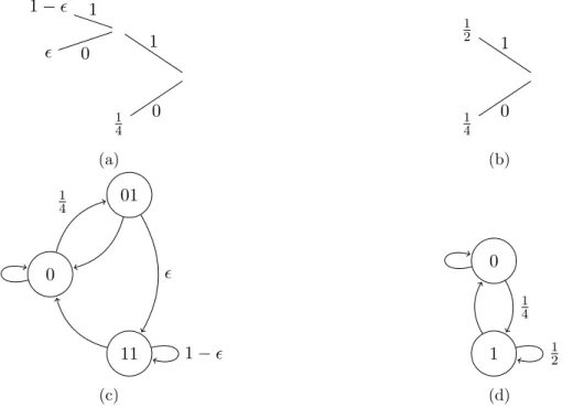
Example 6 LetpT be a Markov process withA={0,1} andT ={0,01,11}, wherep(1|11) =

1−, p(1|01) = , and p(1|0) = 1₄. Figure 3.2 depicts the original and aggregated processes as context trees and state transition diagrams. Calculating the stationary distribution of pT yields π(11) =π(01) = 1₆ andπ(0) = 2₃. Then the aggregated processpT˜, where ˜T ={0,1}, has ˜p(1|0) = 14

and ˜p(1|1) = (1₆ + (1−)1₆)/(1₆ +1₆) = 1₂. If 1

n, then with high probability a sample from pT will show only a subset of the states. However, the aggregate processes is fast mixing and therefore samples from each will look different.

1− ₁ 0 1 1 4 0 (a) 1 2 ₁ 1 4 0 (b) 0 01 11 1 4 1− (c) 0 1 1 4 1 2 (d)

Figure 3.2: (3.2a) States and transition probabilities for Markov process from Example 6. (3.2b) Aggregated process withk= 1. (3.2c) State transition diagram for Markov process from Example 6. (3.2d) Aggregated process withk= 1.

(23)

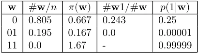
Table 3.1: Empirical frequencies and stationary probabilities of original process for Example 6.

w #w/n π(w) #w1/#w p(1|w)

0 0.805 0.667 0.243 0.25

01 0.195 0.167 0.0 0.00001

11 0.0 1.67 - 0.99999

Table 3.2: Empirical frequencies and stationary probabilities of aggregate process for Example 6.

w #w/n π(w) #w1/#w p(1|w)

0 0.672 0.667 0.239 0.25

1 0.328 0.333 0.509 0.5

3.1 and 3.2 compare the empirical frequencies with the stationary probabilities for the true and aggregate processes. Also displayed are the transition probabilities and their estimates, which will be discussed further in the following sections. In the sample from the original process, the empirical frequencies are not very close to the stationary probabilities and we only see the states 0 and 01. On the other hand, in the sample from the aggregate process, the empirical frequencies are close to their respective stationary probabilities. Additionally, note that in this sample we see occurrences of 0, 01, and 11, which is something that did not happen in the original slow mixing process.

3.3

Difficulties in Estimation

The following examples serve to illustrate some of the problems encountered when estimating processes with memory without making assumptions on the mixing.

Regardless of sample size, it is possible to have states with high stationary weight that do not appear in a sample and for the sample to be composed of strings that have very small stationary weight.

Example 7 Let A = {0,1} and T = {00,01,10,11}, with p(1|00) = _m, p(1|01) = 1 −,

p(1|10) = 1−, and p(1|11) = . Figure 3.3 shows the state transition diagram for the process. For m > > 0, the model pT represents a stationary ergodic Markov process with stationary

distribution π(00) = _mm₊₃ and π(01) = π(10) = π(11) = _m1₊₃. If m is large, then the stationary

(24)

close to 0. Suppose we have a length-nsample and 1

n. If the process starts in one of 01, 10, or 11, then with high probability we will not encounter two or more consecutive zeros.

00 01 10 11 m 1− 1−

Figure 3.3: State transition diagram for Markov process from Example 7.

Note that the process in Example 7 is an example of a slow mixing process. A large number of transitions is needed before the empirical frequncies reflect the stationary probabilities because transitions between certain subsets of states occur with low probability.

This next example from [18] demonstrates that when the memory is unbounded, it may be impossible to distinguish between samples from an i.i.d. process and one with memory.

Example 8 LetpT be a Markov process with memoryk > nand letS(n)be the set of states that

can be reached innsteps when starting from the all zero state. In other words,S(n)is the set of all

states that start with n0’s. Now let p(1|s) = 1₂ for all s∈S(n) and p(1|s) = 1−for all s6∈S(n). Then a length-nsample obtained by starting from the all zero state will be indistinguishable from

a length-nsample generated by an i.i.d. Bernoulli 1₂ process.

The following example illustrates some of the difficulties encountered as a result of the mixing properties of the source.

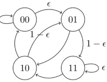
Example 9 Let pT be as in Example 7. Now let T0 = {00,01,10,11}, with p0(1|00) = , p0(1|01) = 1−, p0(1|10) = 1−, and p0(1|11) = . The corresponding state transition is shown in Figure 3.4. For m > > 0, this model represents a stationary ergodic Markov process with stationary distribution π0(00) = π0(01) = π0(10) = π0(11) = 1₄. Recall from Example 7 that

π(00) = _mm₊₃ and π(01) = π(10) = π(11) = _m1₊₃, which varies significantly from π0 when m is

large. Suppose we have a length-n sample and 1

(25)

probability we will see a length-n string like . . .011011011. . .. In either case, the samples from both processes look identical, which means that no estimator would be able to distinguish between the two sources or obtain the correct stationary probabilities.

00 01 10 11 1− 1−

Figure 3.4: State transition diagram for Markov process from Example 9.

Further examples regarding the estimation of Markov processes in the slow mixing setting can be found in [1].

3.4

Conditional Probability Estimate

In what follows we consider estimating the transition probabilitiesp(a|w) in a few simple situations.

3.4.1 Memory

One scenario in which we can obtain good estimates for some transition probabilities is if we know that the memory of the underlying process is less than some D. Then the subsequence following any length-Dor longer contextw is i.i.d. and ˆp(a|w) = #_#w_wa is a reasonable estimate. Since there is no assumption on the mixing, it is possible that the state space has not been fully explored and therefore we can only provide estimates for states that have appeared sufficiently many times.

3.4.2 Mixing

On the other hand, if we had no knowledge of the memory, but we knew that the process had mixed, then we would still be able to obtain good estimates. Since the empirical counts of the strings reflect their stationary weights, then #w_na and #_nw are reasonable estimates of p(wa) and

(26)

p(w), respectively, and ˆp(a|w) = #_#w_wa is a reasonable estimate of p(a|w) = p_p(₍w_wa₎). With the additional information of how close the stationary probabilities and empirical frequencies are, we could also bound the accuracy of the estimate.

3.4.3 Continuity Condition

Without any assumptions on the memory or the mixing of the source, the problem is ill-posed and it is not possible to say anything about our estimates. To be able to proceed further, we adopt a continuity condition as in [17] and [1]. Letd:N+→R+be the continuity condition and letMdbe the set of all models that satisfy for all u∈ {0,1}∗ _and_{a, b, b}0_{∈ {}₀_,₁_}_,

p(a|bu) p(a|b0_u₎ −1 ≤d(|u|). (3.1)

Just as in [1] we require that

X

i≥1

d(i)<∞. (3.2)

What (3.1) says is that the ratio of conditional probabilities given contexts that differ only in the least recent bit are bounded below by 1−d(i) and above by 1 +d(i), whereiis the length of the matching part of the context. In other words,d(i) controls how much the last bit of a context of lengthi+ 1 can affect the conditional probability. Ifd(i) = 0 for alli > D, then we can see that the conditional probabilities for all contexts that differ only after the firstDbits are equal and the process has memoryD.

Requiring (3.2) means that as context length increases, the amount that the last bit can in-fluence the conditional probability decreases. So the continuity condition can be thought of as a soft constraint on the memory of the process. From an information theoretic perspective, we are requiring that the conditional mutual information I(X0;X−i|X₋−₍1_i₋₁₎) decreases asi increases. Equivalently, two bits, given all the bits between, say less about each other the farther apart they are. The following example from [1] illustrates that this condition does not at all constrain the mixing of the process.

(27)

i >1, since our process has only one bit of memory. However,can be chosen arbitrarily small to

make the process slow mixing.

3.5

Bound on the Conditional Probability Estimate

Given a sample X1, X2, . . . , Xn obtained from an unknown source pT belonging to the class Md, Theorem 2 from [1] provides deviation bounds on the estimates of the conditional probabilities. Let k=|w|, where w is the context of interest and let δk =

P

i≥kd(i). With probability at least

1− 1 22klogn, #w1 #w −p(1|w) ≤ s 2k_log_n₊_nδ k #w . (3.3)

The first term of the bound increases with the length of the context and reflects the intuitive difficulty of providing good estimates with longer contexts. On the other hand, notice that the second term decreases with increasing context length. This is because the aggregated state will be closer to the true state of the process and will therefore have less bias. Also, we can see that simply having a larger sample does not ensure that our estimates will be better, since the terms in the numerator also increase with sample size. Since this result does not depend on the empirical frequencies of states being close to their stationary probabilities, nothing can necessarily be said about shorter contexts from longer ones.

3.6

Slow Mixing Simulations

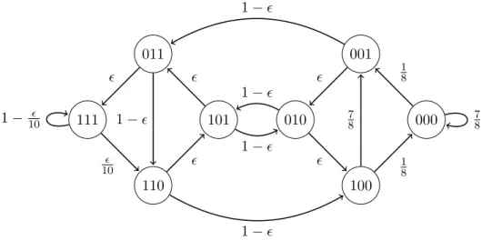
We construct a slow mixing Markov process and generate samples to illustrate some of the curious artifacts we previously mentioned. The binary Markov process has memory D and generates bits using p(1|X−∞−1 ) =q(X−−31) + min{q,1−q}PD−3 i=1 (1−2X−i−3)α(i) 2PD−3 i=1 α(i) (3.4) where q(000) = 1₈,q(001) = 1−,q(010) = 1−, q(011) =,q(100) = 7₈,q(101) = , q(110) =,

q(111) = 1−₁₀, andα(i) = _i12. Figure 3.5 depicts the state transitions for the process given by just the values ofq, i.e., for D= 3. For sufficiently small, the process is slow mixing. We set up the process this way so that all the states with the same three most recent bits (X₋−₃1) have transition

(28)

probabilities that are more similar for longer matching contexts. This allows the process to satisfy the continuity condition. The probabilities corresponding to the three most recent bits are chosen so that the probability of certain transitions can be made arbitrarily small to make the process slow mixing.

We take D= 15,= 10−5 and generate a sample of lengthn= 1000. Our resulting continuity

condition remainsd(i) =O(_i12). For contexts of lengthk∈ {1,2,4,7,10}, we examine the empirical and theoretical stationary and transition probabilities of states that appear sufficiently many times.

101 011 111 110 010 100 000 001 1− 1− 10 1− ₁₀ 1− 1− 1 8 7 8 7 8 1 8 1−

Figure 3.5: State transition diagram of base transition probabilities for slow mixing process (3.4)

Table 3.3 shows the empirical frequencies and stationary probabilities of some strings and their suffixes. Due to the slow mixing nature of the process, the empirical frequencies in general do not reflect the stationary probabilities. However, it is not uncommon to see the longer strings’ counts sometimes reflect their stationary probabilities better than those of their suffixes.

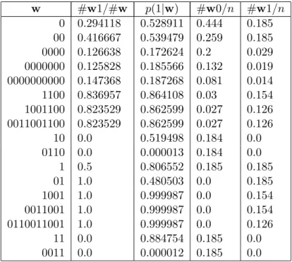
The transition probability estimates and the true transition probabilities given the context w

are displayed in Table 3.4. In some cases the estimates for longer contexts can be better than the estimates for their suffixes. While the common intuition is that it is more difficult to estimate when there is less data, this is countered by the fact that longer contexts are closer to the true state and are therefore less biased.

Recall our earlier comment about how it is important to remember that we are estimating parameters of an aggregated source with samples from the original source, since samples from the two, in general, are not similar. Here we can see that the original process given by (3.4) is slow

(29)

Table 3.3: Empirical and theoretical stationary probabilities for select states of process (3.4) w #w/n π(w) 0 0.629 0.2678 00 0.444 0.126158 0000 0.229 0.048849 0000000 0.151 0.02706 0000000000 0.095 0.014575 1100 0.184 0.068059 1001100 0.153 0.058809 0011001100 0.153 0.058806 10 0.184 0.141642 0110 0.184 0.068059 1 0.37 0.7322 01 0.185 0.141642 1001 0.154 0.058811 0011001 0.154 0.058809 0110011001 0.126 0.050727 11 0.185 0.590557 0011 0.185 0.068059

Table 3.4: Empirical and theoretical transition probabilities for select states of process (3.4)

w #w1/#w p(1|w) #w0/n #w1/n 0 0.294118 0.528911 0.444 0.185 00 0.416667 0.539479 0.259 0.185 0000 0.126638 0.172624 0.2 0.029 0000000 0.125828 0.185566 0.132 0.019 0000000000 0.147368 0.187268 0.081 0.014 1100 0.836957 0.864108 0.03 0.154 1001100 0.823529 0.862599 0.027 0.126 0011001100 0.823529 0.862599 0.027 0.126 10 0.0 0.519498 0.184 0.0 0110 0.0 0.000013 0.184 0.0 1 0.5 0.806552 0.185 0.185 01 1.0 0.480503 0.0 0.185 1001 1.0 0.999987 0.0 0.154 0011001 1.0 0.999987 0.0 0.154 0110011001 1.0 0.999987 0.0 0.126 11 0.0 0.884754 0.185 0.0 0011 0.0 0.000012 0.185 0.0

(30)

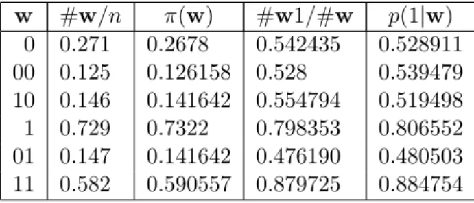
Table 3.5: Empirical and theoretical stationary and transition probabilities for select states of aggregate process w #w/n π(w) #w1/#w p(1|w) 0 0.271 0.2678 0.542435 0.528911 00 0.125 0.126158 0.528 0.539479 10 0.146 0.141642 0.554794 0.519498 1 0.729 0.7322 0.798353 0.806552 01 0.147 0.141642 0.476190 0.480503 11 0.582 0.590557 0.879725 0.884754

mixing, but the aggregated model with memory k = 2 is not. To show how samples from the two processes can differ, we generate a length n = 1000 sample from the memory-2 aggregate source and compare the estimates. Table 3.5 displays the estimates of the stationary and transition probabilities for the sample from the aggregate process, along with the true values. Observe that the estimates of both the stationary and transition probabilities are close to their true values, whereas in the original process, this is not the case.

(31)

Chapter 4

The Jackknife Variance Estimate

We apply a modification of the jackknife procedure to obtain an estimate of the variance of the conditional probability estimates and give bounds on the bias of the jackknife variance estimate, which we first presented in [18]. The theorem in this chapter gives a slightly improved bound.

4.1

Jackknife Procedure for the Variance of

#_#w_w1

Here we describe a natural adaptation to the classical jackknife procedure for estimating the vari-ance when our statistic of interest is the conditional probability of the aggregated process given some context.

LetY1, Y2, . . . , Ym be the subsequence following the contextw, wherem is the number of timesw appears in the sample. From [1], we know that it is reasonable to estimate p(1|w) with

ˆ

Y = Y1+Y2+· · ·+Ym

m . (4.1)

Note that the mean ˆY is the same as #_#w_w1. Then in the same manner as the i.i.d. jackknife, we

sequentially remove samples to obtain the recalculated means,

ˆ

Yi =

Y1+· · ·+Yi−1+Yi+1+· · ·+Ym

(32)

Let ˆY(·) = _m1 Pmi=1Yˆi be the average of the recalculated means. Then the jackknife estimate of Var( ˆY) is VarJack = m−1 m m X i=1 ( ˆYi−Yˆ(·))2. (4.3)

Remark Note that for everything that follows, VarJack denotes the jackknife estimate of the

variance of #_#w_w1, the empirical estimate of the probability of 1 given the length-k context of

con-sideration w. As we do not deviate from the above setting, we drop further references to w.

Proposition 1 VarJack= 1 m(m−1) m X i=1 (Yi−Yˆ)2. (4.4)

Proof Rewriting in terms ofYj’s and simplifying, we can see that

ˆ Yi−Yˆ(·)= P j6=iYj m−1 − Pm i0₌₁P_j₆₌_i0Y_j m(m−1) = −mYi+Pmj=1Yj m(m−1) = ˆ Y −Yi m−1,

and inserting into (4.3) gives the result.

4.2

Bias of the Jackknife Estimate

Here we show how the equation for the jackknife estimate of the variance in Proposition 1 can be obtained by applying the bias correction (2.2) to the naive empirical variance estimate. We have our statistic ˆ θ(Y₁m) = Pm i=1(Yi−Yˆ)2 m , so ˆθi = _m1₋₁P_j6=i(Yj−Yˆi)2 and ˆθ(·)= _m1 Pm

i=1θˆi, where ˆYi is as in (4.2). Then calculating the bias

corrected estimate gives the unbiased estimate for the variance ofYi,

mθˆ(Y₁m)−(m−1)ˆθ₍·)= Pm

i=1(Yi−Yˆ)2

(33)

To obtain the variance estimate of ˆY for i.i.d. Yi’s see that Var( ˆY) = Var 1 m m X i=1 Yi = 1 m2 m X i=1 Var(Yi) + 1 m2 m X i=1 X j6=i Cov(Yi, Yj) = 1 m2 m X i=1 Var(Yi) = 1 mVar(Yi)

where the last two lines follow from the independence and identical distribution of theYi’s, respec-tively. Therefore, for the i.i.d. case, we have the unbiased jackknife estimate of the variance

VarJack= Pm

i=1(Yi−Yˆ)2

m(m−1) .

In our Markov setting, we have that theYi’s may be correlated, and the true state generating each may be different, so our estimate is not unbiased. We analyze the bias in Theorem 4 where we decompose the Yi’s into one set of random variables which form a martingale difference sequence and another which is well behaved.

4.3

Bound on the Jackknife Variance Estimate

Let T be the set of states of the unknown process p, and let Tw = {s ∈ T : w ≺ s} be the set

of true states corresponding to aggregated statew. We are examining the conditional probability for the context w, while each bit in the subsequence is generated by some states that has w as a suffix. Therefore, we want to bound the difference between the two probabilities, and the continuity condition allows us to do so.

Proposition 2 Forδk ≤1 anda∈ {0,1},w∈ {0,1}k, and s∈ Tw,

(34)

Proof From [1] we have forδk≤1, (1−δk) max s∈Tw p(a|s)≤p(a|w)≤ 1 1−δk min s∈Tw p(a|s)

Taking the left inequality we get (1−δk)p(a|s) ≤ p(a|w). Rearranging gives p(a|s)−p(a|w) ≤

p(a|s)δk≤δk, where the last inequality follows because, as a probability,p(a|s)≤1. From the right side inequality we have,p(a|w)≤ p₁(₋a|_δs)

k, and similar to the left side we can see (1−δk)p(a|w)≤p(a|s)

and p(a|w)−p(a|s)≤p(a|w)δk≤δk.

Definition 1 Let 1i(s) be the indicator function that the state corresponding to theith appear-ance of wis s. LetWi=Ps∈Tw1i(s)p(1|s) and letZi =Yi−Wi.

In other words,Wi is the probability of 1 given the true contextsthat generatedYi. TheZi’s form a martingale difference sequence, which has the following properties.

Lemma 1 LetFi denote the sigma algebra of Z1, . . . , Zi. For i < j,

E[Zj|Fi] = 0

and

E[ZiZj] = 0.

Proof For the first part we show that E[Zi |Z1i−1] = 0 for all i. LetSi be the true state of the process that corresponds to the ith appearance of w. Then

E[Zi|Z1i−1] =ESi[E[Zi |Z i−1 1 , Si]] =ESi[E[Yi−Wi|Z i−1 1 , Si]] =ESi[E[p(Yi |Si)]−p(1|Si)] =ESi[p(1|Si)−p(1|Si)] = 0.

(35)

The first two equalities follow by conditioning on the true stateSi and by the definition ofZi. The third follows by the Markov property and definition of Wi and the fourth by evaluating the inner expectation.

The second part follows from conditioning on Fi and applying the first part,

E[ZiZj] =E[E[ZiZj | Fi]] =E[ZiE[Zj | Fi]] =E[Zi·0] = 0.

Proposition 3 Forδk ≤1 and allm >0,

1 m m X i=1 Wi ! −p(1|w) ≤δk.

Proof We have that Pm

i=1 P

s∈Tw1i(s) = m, since the inner summation evaluates to 1. Then

1 m Pm i=1Wi = 1 m Pm i=1 P

s∈Tw1i(s)p(1|s) is a convex combination of the probabilitiesp(1|s), where

s∈ Tw, so applying Proposition 2 gives us the result.

Here we give two lemmas that will be useful in bounding the variances and covariances.

Lemma 2 For any random variableX with|X| ≤,

Var[X]≤2.

Proof Since |X|2 _≤ 2 _{and Var[}_X_{] =} _E_[_X2_]₋_E_[_X_]2_{, we know that 0} _≤ _E_[_X2_] _≤ 2 _and

0≤E[X]2 ≤2. ThereforeE[X2]−E[X]2≤2.

Lemma 3 For any two random variablesU and V,

(36)

Proof By the Cauchy-Schwarz inequality,

|Cov(U, V)|=|E[(U −E[U])(V −E[V])]| ≤pE[(U−E[U])2_]_E_[(_V ₋_E_[_V_])2_]

=pVar[U]Var[V].

Now we give the theorem bounding the bias of the jackknife variance of ˆY.

Theorem 4 Forδk ≤1,

E[VarJack|m]−Var[ ˆY|m] ≤δ 2 k+ 2δk √ m + 2δk m−1

Proof The bound comes from decomposing theYi’s intoWi’s andZi’s, explicitly calculating the bias, and then bounding the resulting covariance terms.

Let ˆW = _m1 Pm i=1Wi and ˆZ= _m1 Pmi=1Zi. Define ˜ Z = 1 m2 m X i=1 E[Z_i2|m]. (4.5) First we have, Var[ ˆY|m] = Var[ ˆW + ˆZ|m]

= Var[ ˆW|m] + Var[ ˆZ|m] + 2Cov( ˆW ,Zˆ|m). (4.6)

Now see that

(37)

where the second line follows because by Lemma 1E[ZiZj|m] = 0 and

E[Zi|m] =E[E[Zi|Fj, m]] = 0. Then for the variance of ˆY, we have

Var[ ˆY|m] = Var[ ˆW|m] + ˜Z+ 2Cov( ˆW ,Zˆ|m). (4.8)

Next, from Proposition 1 and since Yi−Yˆ = (Wi−Wˆ) + (Zi−Zˆ), we have

E[VarJack|m] = E m X i=1 (Yi−Yˆ)2 m m(m−1) = m X i=1 E h (Wi−Wˆ)2 m i + 2E h (Wi−Wˆ)(Zi−Zˆ) m i +E h (Zi−Zˆ)2 m i m(m−1) (4.9)

Taking the term with onlyZi’s we can see that

where the third equality follows as a result of lemma 1. Therefore, for the expected variance estimate, we have E[VarJack|m] = 1 m(m−1) m X i=1 E h (Wi−Wˆ)2 m i + 2 m(m−1) m X i=1 E h (Wi−Wˆ)(Zi−Zˆ) m i + ˜Z. (4.12)

(38)

Taking the difference between (4.12) and (4.6), the ˜Z’s cancel and we are left with

E[VarJack|m]−Var[ ˆY|m]

= 1 m(m−1) m X i=1 E h (Wi−Wˆ)2 m i + 2 m(m−1) m X i=1 E h (Wi−Wˆ)(Zi−Zˆ) m i −Var[ ˆW|m]−2Cov( ˆW ,Zˆ|m). (4.13)

Similarly for the sample variance term,

Pm i=1E h (Wi−Wˆ)2 m i m(m−1) = 1 m(m−1) m X i=1 E W_i2− 2 m m X j=1 WiWj+ 1 m2 m X j=1 m X k=1 WjWk m = 1 m(m−1) m X i=1 E[W_i2|m]− 1 m2₍_m₋₁₎ m X i=1 m X j=1 E[WiWj|m] = 1 m2 m X i=1 E[W_i2|m]− 1 m2₍_m₋₁₎ m X i=1 X j6=i E[WiWj|m]. (4.15)

(39)

and returning to (4.13) we have,

E[VarJack|m]−Var[ ˆY|m]

=− m X i=1 X j6=i Cov(Wi, Wj|m) m(m−1) + 2 m X i=1 Eh(Wi−Wˆ)(Zi−Zˆ) m i m(m−1) −2Cov( ˆW ,Zˆ|m) (4.16) Now we can bound each of the terms. For the second one we can apply the Cauchy Schwarz inequality to show E Pm i=1(Wi−Wˆ)(Zi−Zˆ) m m ≤ E s Pm i=1(Wi−Wˆ)2 m Pm i=1(Zi−Zˆ)2 m m ≤ s E hPm i=1(Wi−Wˆ)2 m m i E hPm i=1(Zi−Zˆ)2 m m i ≤ r δ2 k m−1 m ≤δk (4.17)

where the first inequality uses the regular form |P

aibi| ≤

q P

a2_i P

b2_i and the second uses the

(40)

that is, adding a constant toWi doesn’t change the sample variance. Then since|Wi−p(1|w)| ≤δk the same reasoning as in the proof of Lemma 2 can be applied. Also from (4.10),EPm_i₌₁(Zi−Zˆ)2

m m = m−1 m2 Pm i=1E[Zi2|m]≤ m −1 m , since Z 2 i ≤1.

Now we bound the other terms. By Lemma 2 and Proposition 2,

Var[Wi|m] = Var[Wi−p(1|w)|m]≤δk2. (4.18)

Similarly, by Lemma 2 and Proposition 3,

Var[ ˆW|m] = Var[ ˆW −p(1|w)|m]≤δ_k2. (4.19)

From (4.7) and since|Zi| ≤1,

Var[ ˆZ|m] = 1 m2 m X i=1 E[Z_i2|m]≤ 1 m. (4.20)

Then by Lemma 3 with (4.18) we have

|Cov(Wi, Wj|m)| ≤

q

Var[Wi|m]Var[Wj|m]≤δk2 (4.21)

and with (4.19) and (4.20),

Cov( ˆW , ˆ Z|m) ≤ q Var[ ˆW|m]Var[ ˆZ|m]≤ r δ2 k 1 m = δk √ m. (4.22)

(41)

Then applying (4.17), (4.21), and (4.22) to (4.16), we have

E[VarJack|m]−Var[ ˆY|m] ≤ 1 m(m−1) m X i=1 X j6=i δ_k2+ 2 m−1δk+ 2 δk √ m =δ2_k+ 2δk m−1+ 2δk √ m, (4.23)

finishing the proof of the theorem.

Recall that δk → 0 as k→ ∞. We can see that the bias of the variance estimate decreases as the context length increases. If the context length is longer than the memory of the source, then we have δk = 0 and the subsequenceY1m is i.i.d., resulting in an unbiased estimate. In contrast to

the bound on the transition probability estimate (3.3), there is no term that increases with context length. However, for longer contexts, we will have smaller m, implying a larger bias. Notice that even if we let m → ∞, we still have δ_k2. This term comes from the covariance between Wi’s and remains because we do not know the true states and are instead using an aggregated statew.

(42)

Chapter 5

The Bootstrap Variance Estimate

Here we apply the bootstrap procedure to estimate the variance of the conditional probability estimates. We see how the bootstrap relates to the jackknife for these estimates and obtain a bound on the bias of the bootstrap estimate.

5.1

Bootstrap Variance of

#_#w_w1

Recall that Y1, Y2, . . . Ym is the subsequence following the context w, and the empirical estimate of the conditional probability p(1|w) is ˆY = _m1 Pm

i=1Yi. We want to use bootstrap to obtain an estimate of the variance of ˆY.

We could apply the Monte Carlo algorithm to produce an estimate of the variance. Generating i.i.d. samples Y_i∗b, b = 1. . . B, i= 1. . . m, where Y_i∗b is Bernoulli with P r(Y_i∗b = 1) = ˆY, gives bootstrap replications ˆY∗b= _m1 Pm

i=1Yi∗b and variance estimate

1 B−1 B X b=1 ( ˆY∗b−Yˆ∗•)2 where ˆY∗•= _B1 PB b=1Yˆ ∗b_.

However, this is unnecessary as we are able to perform the calculations for the variance. Let VarBoot denote the bootstrap estimate of the variance of ˆY. Then we have

(43)

Note that just like in the jackknife case, the variance estimate here is based on the samples being i.i.d. As they are not, we analyze the correlations betwen Yi’s to provide a bound on the bias.

5.2

Bootstrap vs. Jackknife Estimate

We can see that the bootstrap estimate proposed above is actually a scaling of the estimate resulting from the earlier jackknife procedure,

VarBoot= 1 m( ˆY −Yˆ 2₎ = 1 m 1 m m X i=1 Yi− 1 m2 m X i=1 m X j=1 YiYj = 1 m 1 m m X i=1 Yi− 2 m2 m X i=1 m X j=1 YiYj+ 1 m3 m X i=1 m X j=1 m X k=1 YjYk = 1 m2 m X i=1 (Yi−Yˆ)2 =m−1 m 2_Xm i=1 ( ˆYi−Yˆ(·))2 = m−1 m VarJack.

This also means that in the i.i.d. case, the bootstrap variance is biased downwards,

E[VarBoot] =

m−1

m Var( ˆY).

5.3

Bound on the Bootstrap Variance Estimate

Similar to the section on jackknife, we bound the bias of the bootstrap variance for the conditional probability estimates.

Theorem 5 Forδk ≤1,

E[VarBoot|m]−Var[ ˆY|m] ≤δ 2 k+ 2δk √ m + 2δk m + 1 m2.

(44)

Proof We take the same approach as in the proof of the jackknife bias for obtaining the bound.

From (4.6) we have

Var[ ˆY|m] = Var[ ˆW|m] + Var[ ˆZ|m] + 2Cov( ˆW ,Zˆ|m). (5.2)

and scaling (4.12) appropriately gives

E[VarBoot|m] = m−1 m E[VarJack|m] = 1 m2 m X i=1 E h (Wi−Wˆ)2 m i + 2 m2 m X i=1 E h (Wi−Wˆ)(Zi−Zˆ) m i +m−1 m Z.˜ (5.3)

Taking the difference of (5.3) and (5.2) gives the bias,

E[VarBoot|m]−Var[ ˆY|m] =

1 m2 m X i=1 E h (Wi−Wˆ)2 m i + 2 m2 m X i=1 E h (Wi−Wˆ)(Zi−Zˆ) m i − 1 mZ˜−Var[ ˆW|m]−2Cov( ˆW ,Zˆ|m), (5.4)

where we can see that the ˜Z’s don’t completely cancel.

Recall from (4.14) that the variance of ˆW is

Var[ ˆW|m] = 1 m2 m X i=1 E[W_i2|m]− 1 m2 m X i=1 E[Wi|m]2+ 1 m2 m X i=1 X j6=i Cov(Wi, Wj|m).

Also recall the sample variance ofWi from (4.15), 1 m2 m X i=1 E h (Wi−Wˆ)2 m i = m−1 m3 m X i=1 E[W_i2|m]− 1 m3 m X i=1 X j6=i E[WiWj|m],

(45)

Returning to (5.4) and substituting (5.5) we obtain

E[VarBoot|m]−Var[ ˆY|m] =−

Now we can use (4.18), (4.21), (4.17), and (4.22) to bound each of the terms in the bias,

|E[VarBoot|m]−Var[ ˆY|m]| ≤

1 m3 m X i=1 δ_k2+m+ 1 m3 m X i=1 X j6=i δ_k2+ 2 mδk+ 1 m 1 m + 2√δk m =δ_k2+2δk m + 1 m2 + 2δk √ m,

(46)

We would expect the bound to be similar to the jackknife one, since the bootstrap estimate is simple the jackkknife estimate scaled by m_m−1. The main difference here is that as we let context

lengthk→ ∞,δk→0, and we are left with _m12. This is because as we saw in the previous section, the bootstrap estimate is biased. Therefore, we would not expect the bias to disappear completely. The rest of the terms remain the same, except we now have 2δk

m instead of

2δk

m−1, due to the scaling

of the estimate. Just as with the jackknife, as m → ∞ the δ2_k corresponding to the variance of and covariance between Wi’s remains, again because we are approximating the true state s with an aggregated state w.

(47)

Bibliography

[1] M. Asadi, R. P. Torghabeh, and N. P. Santhanam, “Stationary and transition probabilities in slow mixing, long memory markov processes,”IEEE Transactions on Information Theory, vol. 60, no. 9, pp. 5682–5701, 2014.

[2] B. Efron, The jackknife, the bootstrap and other resampling plans. SIAM, 1982.

[3] B. Efron and C. Stein, “The jackknife estimate of variance,” The Annals of Statistics, pp. 586–596, 1981.

[4] B. Efron, “Bootstrap methods: Another look at the jackknife,” Ann. Statist., vol. 7, no. 1, pp. 1–26, 01 1979. [Online]. Available: https://doi.org/10.1214/aos/1176344552

[5] M. Stone, “Cross-validatory choice and assessment of statistical predictions,” Journal of the Royal Statistical Society. Series B (Methodological), vol. 36, no. 2, pp. 111–147, 1974. [Online]. Available: http://www.jstor.org/stable/2984809

[6] E. Carlstein, “The use of subseries values for estimating the variance of a general statistic from a stationary sequence,” Ann. Statist., vol. 14, no. 3, pp. 1171–1179, 09 1986. [Online]. Available: https://doi.org/10.1214/aos/1176350057

[7] H. R. Kunsch, “The jackknife and the bootstrap for general stationary observations,” The Annals of Statistics, pp. 1217–1241, 1989.

[8] R. Y. Liu and K. Singh, “Moving blocks jackknife and bootstrap capture weak dependence,”

(48)

[9] D. N. Politis and J. P. Romano, “A general resampling scheme for triangular arrays ofα-mixing random variables with application to the problem of spectral density estimation,”The Annals of Statistics, pp. 1985–2007, 1992.

[10] ——, “A nonparametric resampling procedure for multivariate confidence regions in time series analysis,” inComputing Science and Statistics. Springer, 1992, pp. 98–103.

[11] D. N. Politis, J. P. Romano, and T.-L. Lai, “Bootstrap confidence bands for spectra and cross-spectra,” IEEE Transactions on Signal Processing, vol. 40, no. 5, pp. 1206–1215, 1992. [12] D. N. Politis and J. P. Romano, “The stationary bootstrap,”Journal of the American

Statis-tical association, vol. 89, no. 428, pp. 1303–1313, 1994.

[13] J. L. Horowitz, “Bootstrap methods for markov processes,” Econometrica, vol. 71, no. 4, pp. 1049–1082, 2003.

[14] E. Paparoditis and D. N. Politis, “The local bootstrap for markov processes,” Journal of Statistical Planning and Inference, vol. 108, no. 1, pp. 301–328, 2002.

[15] B. Hansen, “Non-parametric dependent data bootstrap for conditional moment models,” Uni-versity of Wisconsin–Madison working paper, 1999.

[16] P. B¨uhlmann, “Sieve bootstrap with variable-length markov chains for stationary categorical time series,” Journal of the American Statistical Association, 2011.

[17] I. Csisz´ar and Z. Talata, “Consistent estimation of the basic neighborhood of markov random fields,”The Annals of Statistics, pp. 123–145, 2006.

[18] K. Oshiro, C. Wu, and N. P. Santhanam, “Jackknife estimation for markov processes with no mixing constraints,” in 2017 IEEE International Symposium on Information Theory (ISIT), June 2017, pp. 3020–3024.