LSHTM Research Online
Atkinson, AD; (2019) Reference Based Sensitivity Analysis for Time-to-Event Data. PhD thesis, London School of Hygiene & Tropical Medicine. DOI: https://doi.org/10.17037/PUBS.04652901 Downloaded from: http://researchonline.lshtm.ac.uk/4652901/
DOI:https://doi.org/10.17037/PUBS.04652901
Usage Guidelines:
Please refer to usage guidelines at https://researchonline.lshtm.ac.uk/policies.html or alternatively contact [email protected].
Reference Based Sensitivity Analysis
for Time-to-Event Data
ANDREW DAVID ATKINSON
Thesis submitted in accordance with the requirements for the degree of Doctor of Philosophy of the University of London
April 2019
Department of Medical Statistics
Faculty of Epidemiology and Population Health LONDON SCHOOL OFHYGIENE ANDTROPICAL MEDICINE
Declaration
I, Andrew David Atkinson, confirm that the work presented in this thesis is my own.
Where information has been derived from other sources, I confirm that this has been indicated in the thesis.
Signature
Acknowledgements
I would like to take the opportunity to thank my supervisors James Carpenter and Mike Ken-ward of LSHTM for providing the impetus, guidance and support for carrying out the work. In particular, James accompanied me throughout the last 6 years, always on hand with encourage-ment. Despite retiring and moving to Scotland, Mike has continued to offer sage advice and guidance for the work, so special thanks also to him.
On a similar note I would like to thank Suzie Cro, now of Imperial College, for providing an excellent blueprint for the theoretical calculations in Chapter 4, and for painstakingly checking each line of the workings, including those in the appendices.
I would like to thank Tim Clayton and Stuart Pocock of LSHTM for allowing me to use the RITA-2 data set, particularly to Tim for providing cleaned data, and being on hand for my questions.
The analysis in Chapter 5 was partially funded from the Swiss National Science Foundation project number 324730 149792. Accordingly, my heartfelt thanks go to the principle inves-tigator of the project, Hansjakob Furrer of the University Hospital in Bern, the Opportunistic Infections working group of COHERE, and all the cohorts within COHERE for allowing us to use their data. Thanks to Marcel Zwahlen of the University of Bern for numerous challeng-ing discussions of the emulated trial, and to Jonathan Sterne of Bristol University, and Miguel Hernan of Harvard University, for taking the time to review the material in the final chapter. My sincerest gratitude to Jonas Marschall and Hansjakob Furrer of the University Hospital in Bern, and John Van Den Anker, Marc Pfister and Julia Bielicki of the University Children’s Hospital in Basel, for giving me the chance to change direction and work in this challenging field.
Thank you to all the patients for allowing us to use their data in the analyses.
And finally of course, wholehearted thanks to my family Louise, Jennifer and Kate for their continued patience, support and understanding through the numerous ups and downs.
Abstract
The analysis of time-to-event data typically makes the censoring at random assumption, i.e. that — conditional on covariates in the model — the distribution of event times is the same, whether they are observed or unobserved. When patients who remain in follow-up are compliant with the trial protocol, then analysis under this assumption can be considered to address a de-jure
(“while on treatment strategy”) type of estimand.
In such cases, we may well wish to explore the robustness of our inference to more prag-matic,de-facto, (“treatment policy strategy”), assumptions about the behaviour of patients post-censoring. This is particularly the case when censoring occurs if patients change, or revert, to the usual (i.e. reference) standard of care.
Recent work has shown how such questions can be addressed for trials with continuous outcome data and longitudinal follow-up, using reference based multiple imputation. Such an approach has two advantages: (i) it avoids the user specifying numerous parameters describing the dis-tribution of patient’s post-withdrawal data, and (ii) it is, to a good approximation, information anchored, so that the proportion of information lost due to missing data under the primary anal-ysis is held constant across the sensitivity analyses.
We develop similar approaches in the survival context, proposing a class of reference based assumptions appropriate for time-to-event data. We explore the extent to which sensitivity anal-yses using the multiple imputation estimator (with Rubin’s variance formula) is information anchored, demonstrating this using theoretical results and simulation studies. The methods are illustrated using data from a randomized clinical trial comparing medical therapy with angio-plasty in patients with angina.
Causal inference methods are established as the gold standard for analysing observational (“big”) data. In a final step, we show that reference based methods can also be applied in this context by using sensitivity analysis in an investigation of the risk of opportunistic infections in a cohort of HIV positive individuals.
Contents
1 Introduction 1
1.1 Missing data in a clinical trials . . . 1
1.2 Estimands . . . 9
1.3 Regulatory Framework . . . 12
1.4 Statistical methods for analysing time-to-event data . . . 14
1.5 Sensitivity analysis approaches . . . 17
1.5.1 Introduction . . . 17
1.5.2 Selection models . . . 18
1.5.3 Pattern mixture models . . . 19
1.5.4 Shared parameter models . . . 22
1.6 Information Anchoring principle . . . 23
1.7 Summary of motivation for thesis . . . 26
1.8 Multiple Imputation . . . 26
1.9 Reference-based sensitivity analysis methods . . . 34 1.10 Clinically relevant and accessible sensitivity analysis for time-to-event outcomes 40
1.11 Motivating data sets . . . 42
1.11.1 German breast cancer data . . . 42
1.11.2 The RITA-2 Study . . . 42
1.11.3 Observational data from COHERE . . . 43
1.12 Focus of the thesis . . . 43
2 Reference based methods for time-to-event data 45 2.1 Introduction . . . 45
2.2 Defining the post-deviation distribution in terms of other treatment arms . . . . 46
2.3 Imputation under CAR . . . 47
2.4 Proposals for reference based imputation under Censored not at Random (CNAR) 49 2.4.1 Introduction . . . 49
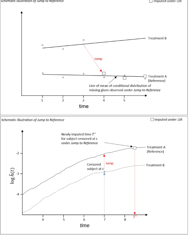
2.4.2 Jump to Reference (J2R) . . . 49
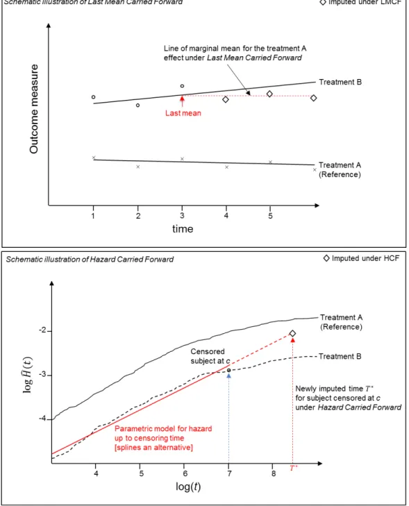
2.4.3 Last Mean Carried Forward / Hazard Carried Forward . . . 52
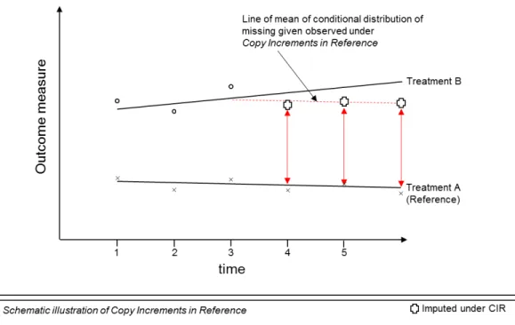
2.4.4 Copy Increments in Reference . . . 55
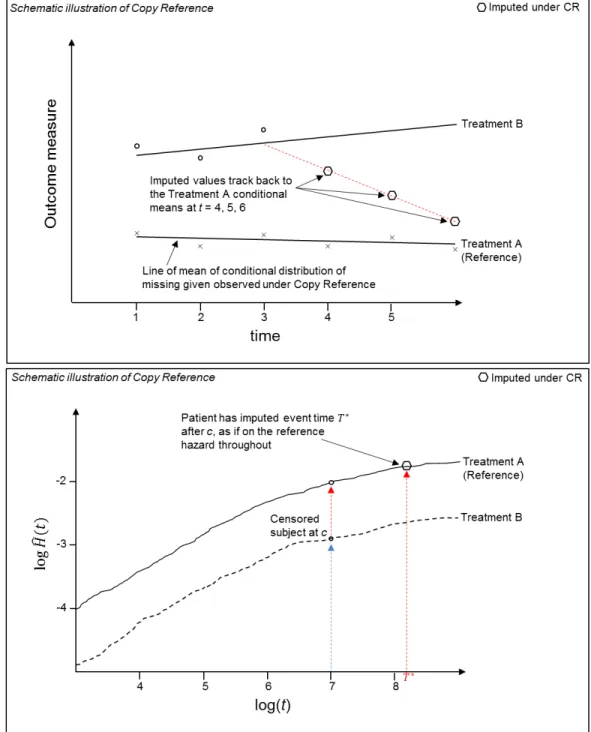
2.4.5 Copy Reference . . . 58
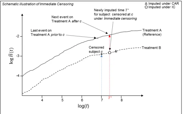
2.4.6 Immediate Event . . . 60
2.4.7 Hazard Increases/Decreases to extremes . . . 62
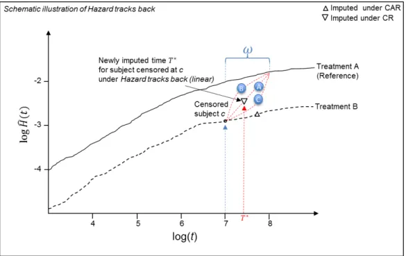
2.4.8 Hazard Tracks Back to reference in time window . . . 64
2.4.9 Delta methods . . . 67
2.5 Summary . . . 70
2.6.1 Introduction . . . 71
2.6.2 Results . . . 73
2.7 Discussion . . . 84
2.8 Application of the sensitivity methods to the German Breast Cancer data . . . . 85
2.8.1 Introduction . . . 85
2.8.2 Model for the data . . . 88
2.8.3 Results from applying the sensitivity analysis methods to the GBC data 89 2.9 Discussion of results . . . 93
2.9.1 Evaluation of methods . . . 93
2.9.2 The proportional hazards assumption . . . 95
2.10 Summary . . . 96
3 Information anchoring for reference based sensitivity analysis with time-to-event data 98 3.1 Introduction . . . 98
3.2 Simulation study . . . 101
3.3 Reference based sensitivity analysis for the RITA-2 Study . . . 108
3.4 Summary . . . 111
4 Behaviour of Rubin’s variance estimator for reference based sensitivity analysis with time-to-event data 114 4.1 Introduction . . . 114
4.2 Clinical trial setting with time-to-event data . . . 115
4.3.1 Variance estimation when data is fully observed . . . 118
4.3.2 Censoring on the active arm . . . 119
4.3.3 Multiple imputation . . . 121
4.3.4 Rubin’s variance estimate under CAR . . . 123
4.3.5 Information ratio under CAR . . . 133
4.4 Information anchoring under Jump to Reference . . . 134
4.5 Simulation study . . . 138
4.5.1 Information anchoring for the RITA-2 data . . . 141
4.6 Summary . . . 144
5 Reference-based multiple imputation to investigate informative censoring: Atrial emulationin COHERE 145 5.1 Preamble — sensitivity analysis born out of necessity . . . 145
5.2 Introduction . . . 147
5.3 Causal methods, trial emulation and the rationale for a different approach to sensitivity analysis . . . 148
5.4 Methods . . . 153
5.4.1 Target trial . . . 153
5.5 Emulated trial using COHERE data . . . 155
5.6 Emulation of multiple trials . . . 159
5.7 Statistical methods . . . 161
5.7.1 Analysis model: Estimating the observational analogue of the per-protocol effect . . . 161
5.7.2 Inverse probability weighting to account for covariate dependent
cen-soring . . . 164
5.7.3 Sensitivity analysis . . . 167
5.8 Results . . . 169
5.8.1 Clinical endpoints . . . 169
5.8.2 Sensitivity analysis to investigate informative censoring . . . 176
5.8.3 Subgroup analyses . . . 178
5.9 Summary . . . 180
6 Discussion 182 6.1 Sensitivity analysis for time-to-event data . . . 182
6.2 Reference based sensitivity analysis using multiple imputation . . . 183
6.3 Information anchored sensitivity analysis . . . 185
6.4 Observational data example . . . 186
6.5 The “best” approach to sensitivity analysis . . . 189
6.6 Joint and shared parameter models . . . 190
6.7 Software implementations and adoption . . . 191
6.8 Final remarks . . . 191
A German Breast Cancer Data set 195 A.1 Exploratory Data Analysis . . . 195
C Adapted variance calculation for the truncated normal distribution 204
D Rubin’s variance estimate under the de-jure estimate of CAR 205
E Proof of Lemma 1 regarding variance inflation under CAR 220
F Design based variance estimator when post-deviation data is observed for the
de-facto estimand 222
G Rubin’s variance under thede-factoassumption of Jump to Reference (J2R) 226
H Proof for information anchoring property for Jump to Reference 233
I Survival function for the pooled logistic model 239
J PCP risk models 242
K Inverse probability weights 244
K.1 Inverse Probability Weights . . . 244 K.2 Patient example . . . 247
L Sensitivity analysis for the PCP study 249
L.1 Multiple imputation under Censoring at Random . . . 249 L.2 Sensitivity analysis using “Jump to Reference” approach . . . 255 L.3 Algorithm . . . 255
List of Tables
1.1.1 Summary of review articles on missing data . . . 4
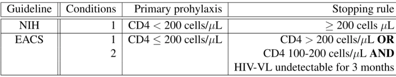
1.11.1NIH and EACS guidelines for PCP prophylaxis . . . 43
2.8.1 Treatment combinations and their censoring levels . . . 85
2.8.2 Sensitivity methods applied to GBC data . . . 91
2.9.1 Comparison of sensitivity analysis methods . . . 95
3.2.1 Simulation results . . . 106
3.3.1 RITA-2 analysis . . . 110
4.5.1 Difference between Rubin’s Jump to Reference MI variance estimator and the information anchored variance estimate . . . 140
4.5.2 Descriptive statistics for the RITA-2 data set and variance estimator comparisons 143 5.4.1 Target trial and emulated trial using observational data from COHERE. . . 154
5.5.1 Characteristics for eligible COHERE patients . . . 158
5.8.1 Estimates from fitting a pooled logistic regression model for the primary analysis 170 5.8.2 Estimates from fitting a pooled logistic regression model for the all-cause mor-tality endpoint . . . 172
5.8.3 Results summary . . . 174 5.8.4 Results summary for Trials A and B . . . 179
List of Figures
1.9.1 Information anchoring example . . . 37
2.4.1 Illustrative example of Jump to Reference . . . 51
2.4.2 Illustrative example of Last Mean Carried Forward / Hazard Carried Forward . 53 2.4.3 Illustrative example of Copy Increments in Reference . . . 56
2.4.4 Illustrative example of Copy Reference . . . 59
2.4.5 Illustrative example of Immediate Event . . . 61
2.4.6 Illustrative example of Extreme Hazard Increasing/Decreasing . . . 63
2.4.7 Illustrative example of Hazard Tracks Back . . . 66
2.4.8 Illustrative example of the delta method . . . 69
2.6.1 Comparison of empirical and theoretical results for Jump to Reference . . . 76
2.6.2 Simulation results with Immediate Event . . . 78
2.6.3 Illustrative example with Extreme Hazard Increasing . . . 80
2.6.4 Illustrative example with Extreme Hazard Increasing . . . 81
2.6.5 Illustrative example with Hazard Tracks Back . . . 83
2.8.2 Log cumulative hazard for reference and treatment arms under CAR and J2R . 89 2.8.3 Log cumulative hazard for reference and treatment arms under CAR and EH/I,
EH/D and IE . . . 92
2.8.4 Log cumulative hazard for reference and treatment arms under CAR and HTB . 93 3.2.1 Increase in variance as censoring increases . . . 105
3.2.2 Simulation results . . . 107
3.3.1 RITA-2 trial: Nelson-Aalen survival plots . . . 109
3.3.2 Plot of the cumulative hazard with Nelson-Aalen estimates, from the fitted Weibull model and under “Jump to PTCA arm” . . . 112
5.4.1 Hypothetical target trial . . . 155
5.6.1 Patient examples. . . 161
5.7.1 Schematic illustration of “Jump to Reference” . . . 168
5.8.1 Adjusted hazard ratios (HR) for the PCP diagnosis primary endpoint . . . 171
5.8.2 Adjusted hazard ratios (HR) for the all-cause mortality secondary endpoint . . 173
5.8.3 Hazard ratios (HR) for endpoints PCP diagnosis and all-cause mortality . . . . 175
5.8.4 Comparison of those on and off PCP prophylaxis . . . 177
A.1.1Exploratory data analysis for categorical variables . . . 199
A.1.2Exploratory data analysis for continuous variables . . . 199
A.1.3Event and censoring profile for the data set . . . 200
A.1.4Kaplan-Meier plot of the treatment effect . . . 201
A.1.5Kaplan-Meier estimator of the survival function for the treatment effect without hormonal treatment . . . 201
K.2.1Patient example with covariate data . . . 248
Glossary
CABG Coronary Artery Bypass Graft
CAR Censoring at Random
cART Combination Antiretroviral Therapy CCAR Censoring Completely at Random CIR Copy Increments in Reference CNAR Censoring Not at Random
COHERE Collaboration of Observational HIV Epidemio-logical Research Europe
CPH Cox Proportional Hazards
CR Copy Reference
CROI Conference on Retroviruses and Opportunistic Infections
EH/I Extreme Hazard / Decrease EH/I Extreme Hazard / Increase EM Expectation-Maximisation EMA European Medicines Agency
FDA US Food and Drug Administration
G-T Grambsch-Therneau (test)
GBC German Breast Cancer
HCF Hazard Carried Forward
HR Hazard Ratio
HTB Hazard Tracks Back
ICH International Conference on Harmonisation of Technical Requirements for Registration of Phar-maceuticals for Human Use
IDU Intravenous Drug User
IE Immediate Event
IPW Inverse Probability Weighting IQR Interquartile Range
ITT Intention to treat IV Instrumental Variable
IWHOD International Workshop on HIV and Hepatitis Observational Databases
J2A Jump to Active
J2R Jump to Reference
LMCF Last Mean Carried Forward LOCF Last Observation Carried Forward
MAR Missing at Random
MCAR Missing Completely at Random
MI Multiple Imputation
MMRM Mixed Model Repeated Measures MNAR Missing Not at Random
MSM Marginal Structural Model MVN Multivariate Normal
NRC US National Research Council NRI Non-random Intervention
PCP Pneumocystis Pneumonia PH Proportional Hazards
RCT Randomised Controlled Trial RMST Restricted Mean Survival Time RNA Ribonucleic acid
Chapter 1
Introduction
But, Mousie, thou art no thy-lane [alone], In proving foresight may be vain;
The best-laid schemes o’ mice an’ men
Gang aft agley [askew],
An’ lea’e us nought but grief an’ pain, For promis’d joy!
“To a Mouse, on Turning Her up in Her Nest with the Plough”, Robert Burns, 1785
1.1
Missing data in a clinical trials
However carefully clinical trials are designed and planned, some baseline patient characteristic and — more typically — outcome data are often missing. This might occur when a patient is lost to follow-up, which could be, for example, due to non-compliance with the study protocol, or stopping an assigned treatment due to experiencing adverse effects. Of course, preventive measures, good design and consistent follow-up processes should be pursued to minimise the amount of missing data — since these would make many of the issues discussed here obsolete (LaVange and Permutt (2016) and Chapter 2 of O’Kelly and Ratitch (2014)).
In this thesis we focus primarily on missing outcome information, rather than baseline data, and in particular, such data in a time-to-event setting. Whatever the reason for the data being
miss-ing, review articles of trials suggest that perhaps 90% of trials have some kind of missing data (Woodet al., 2004; Powneyet al., 2014; Bellet al., 2014; Fieroet al., 2016). In observational data settings missing data also arise, often for the same types of reasons as in a clinical trial. As we might expect, in epidemiological studies the picture regarding the levels of missing data is rather similar (Eekhoutet al., 2012).
Missing data cause unavoidable ambiguity in the analysis of data from clinical trials since any such analysis relies on untestable assumptions about the missing data. If a contextually im-plausible assumption concerning the missing data is made, the estimated treatment effect and associated variance will be biased, leading to potentially misleading inferences, which can di-rectly influence patient care (Sterneet al., 2009; White and Carlin, 2010; Ibrahimet al., 2012; Jakobsen et al., 2017). Hence, it is important to be clear about the assumptions being made about the missing data, and the subsequent impact of these assumptions made on the conclu-sions drawn. Typically, we choose a standard set of assumptions about the missing data for the primary analysis of a trial, and then investigate a number of other plausible scenarios concern-ing the missconcern-ing data through a series of further sensitivity analyses. Since the observed data are consistent with different clinical interpretations, the results from the sensitivity analyses are compared with those from the primary analysis. If they are in line with one another, we may conclude that for the sensitivity analysis scenarios investigated, the outcome from the pri-mary analysis is robust to contextually plausible departures from the assumption concerning the missing data mechanism defined for the primary analysis. If this is not the case, and the results change following the sensitivity analysis, then the investigators should report the conditions under which the results may change, along with the relative likeliness of these circumstances occurring. These steps provide more confidence in the results, especially when regulators are considering new treatments for approval.
Despite the ubiquity of missing data, until relatively recently most primary Randomized Con-trolled Trial (RCT) analyses either used only data from patients with complete data, that is, those with fully observed data, or in a longitudinal setting, used methods such as “last observa-tion carried forward”. While both these approaches may lead to unbiased results under certain causes of missing data, and are certainly simple to implement, they are at best inefficient. A complete case analysis may also lead to less variability in treatment estimates, with its as-sociated knock-on effect for the confidence intervals in the results from the trial. Of course, using just the subset of patients with data complete also reduces power, this issue becoming
aggravated as the number of covariates with missing data increases (page 43 of Molenberghs and Kenward (2007)).
As an alternative to just using the complete cases, we may use all the observed data, also known as an “available cases” analysis. A typical example of this is when considering longitudinal data in which all observed follow-up data at any visit is included in the analysis, irrespective of whether data from other visits for a specific subject were missing. The analysis is then based on defining a model for all the observed data and using this for inference, often employing the likelihood function or posterior distribution. This is the main focus of the text by Little and Rubin (2002), and is exemplified by the mixed model repeated measures approach (MMRM) presented in Molenberghs and Kenward (2007). However, we do not consider these approaches further here.
There are a number of possibilities for “filling in”, or imputing, the missing data. We adopt the taxonomy for missing data methods from Little and Rubin (pages 19 and 60 of Little and Rubin (2002)). In terms ofimputation-basedprocedures, perhaps the most obvious process would be to impute theunconditional meanof the respective covariate which is missing.
However, using the mean to impute has the unfortunate consequence that whilst we do not increase the information in the data, we are increasing the number of subjects in the analysis, so that the sample variance actually decreases. This is undesirable since we would like the imputation process to mirror the loss of information from having missing data. A variation on mean imputation is when the conditional mean is used to impute missing values, sometimes called regression imputation. In this case, the missing value is predicted conditional on the observed outcome and covariate values for the patients.Stochastic imputationfollows the same approach, but adds a small amount of error to each imputed value to help with solving the lack of variability mentioned above.
For longitudinal data, a commonly used method is last observation carried forward (LOCF) . In this case, the last observed value is used to impute missing values for later visits without measurements. This has often been assumed to be a conservative approach, but it may equally be anti-conservative. This is the crux of the issue with LOCF — it is sensitive to the clini-cal context. As pointed out by Molenberghs and Kenward for the example of treatments for Alzheimer’s diseases, “the goal is to prevent the patient from worsening. Thus, in a one year trial where a patient drops out after one week, carrying the last observation forward implicitly assumes no further worsening. This is obviously not conservative” (page 53 of Molenberghs
Review article Year % of articles with Complete case single imputation robust
missing data analysis methods methods
Woodet al. 2004 89% 65% 20% 3%
Eekhoutet al. 2012 92% 81% 14% 13%
Powneyet al. 2014 91% 32% 14% 22%
Bellet al. 2014 95% 45% 27% 27%
Fieroet al. 2016 93% 55% 8% 29%
Table 1.1.1: Summary of review articles on missing data
and Kenward (2007)). Despite many examples and the consistent message that using LOCF can lead to biased results (Mallinckrodtet al., 2004; Carpenteret al., 2003; Beunckenset al., 2005), it is often still used as the simplest alternative, particularly in analyses of observational cohort data. There are also other single imputation methods, mostly developed in other settings such as survey analysis. For example, hot deck single imputation fills in missing values with those from people with similar characteristics (Little and Rubin, 2002). Predictive mean matching
is similar to this — values are imputed by finding the “nearest-neighbour” to the individual with missing values, and using this donor’s observed values as substitutes (van Buuren, 2012). All such single imputation methods generally further aggravate problems because the analysis cannot distinguish between actual and imputed values, and so underestimate the variance. Multiple imputation (MI) , the method we use predominantly for the work presented here, essen-tially builds on stochastic imputation by incorporating additional variability into the imputation process. Being Bayesian in nature MI assumes estimates from fitting a model to the observed data are normally distributed and uses a draw from this distribution to inject variability into the imputed data. In a further step following imputation, an additional component is added to the variance calculation to ensure that it is suitably inflated to reflect the information lost from the missing data (MI is defined in more detail later in this chapter). We note at this point that under missing at random (MAR) , the maximum likelihood based approaches (e.g. MMRM) mentioned above, and those involving MI will end up with essentially the same results (up to Monte Carlo error). This can of course be used as a useful cross-check of the MI process prior to investigating more complex missingness mechanisms, assuming a closed form solution for the likelihood function is available.
Table 1.1.1 briefly summarises five review articles of major medical journals showing that de-spite high levels of missingness in trials, very few used statistically valid methods such as
mul-tiple imputation or likelihood based approaches to suitably account for missing data. Nonethe-less, the increase in the number of studies in the period 2004 to 2014 using such methods is striking. This trend mirrors the increase in availability of standard software using more rig-orous methods during this period, which has allowed specialists and non-specialists alike to perform more robust missing data analyses (Rezvanet al., 2015).
This trend is encouraging, showing that the adoption of more reliable methods is possible, if supported with software implementations. Interestingly, the review by Eekhoutet al. referred to in Table 1.1.1 focussed on epidemiological studies, but the results are very similar to the other reviews concerning missing data in trials.
Table 1.1.1 also highlights the importance of defining methods for handling missing data that are not only valid in a statistical sense, but which are also convenient in terms of ease of use: Adoption of new methods is often directly related to simplicity of implementation. This is the first of three key requirements which need to be taken into account when defining new statistical methods:
The first key facet when considering new sensitivity analysis methods is theirpracticality, that is, their ease of implementation and use.
We will define three such key facets in this introductory chapter, and due to their importance, we will refer back to them in the remainder of the thesis as motivation regarding the proposed sensitivity analysis approaches.
There is, however, a potential downside from the uptake of new missing data methods driven by increased use of readily available software. Software implementations often implement a default set of assumptions regarding the missing data. Whilst the standard assumptions of-ten correspond to the most natural starting point, and are certainly the most straightforward to perform quickly, there is a tendency for the user to accept the premise of these standard assumptions without much reflection and consideration of potential alternatives. The missing data analysis using the standard set of assumptions often stops at this point, without exploration of what would have happened with other, perhaps more tenable scenarios, in the context of a specific trial. Framing these other scenarios so that they are i. clinically plausible, ii. accessible
in terms of the assumptions made, and iii.) relatively easy to be implemented, is the focus of this thesis.
To help us think about missing data, and the different assumptions that might be applicable for such data, it is often helpful to consider the potential relationship between the observed data and missing data. A common framework for such assumptions was proposed by Little and Rubin (e.g. page 12 of Little and Rubin (2002)), and these may be used to provide the foundation for the assumptions underlying the primary and subsequent sensitivity analyses with regards to missing data. Little and Rubin proposed these definitions for different types of missing data, and these have also been adopted for medical settings.
LetY = (yi,j)be a (n×K) rectangular data set with theith rowyi =yi,1, . . . , yi,K whereyi,j
is the value of theyjth variable for subjecti. Define the missing data matrixM = (mij), such
thatmi,j = 1ifyi,jis missing andmi,j = 0ifyi,jis observed. M defines thepatternof missing
data.
The missing data mechanism may be defined by the conditional distribution ofM givenY, say f(M|Y,φ), whereφare the unknown parameters of this distribution.
Now, if missingness does not depend on the values of the dataY,missingorobserved, so that f(M|Y,φ) = f(M|φ) for allY,φ, (1.1.1) then the data are missing completely at random (MCAR) . The missingness in this case does not depend on the data values at all.
Now, letYobsbe the observed data, andYmisbe the values that are missing.
If the missingness depends only on theYobs, but not on theYmis, then the missing data
mecha-nism is said to bemissing at random(MAR),
f(M|Y,φ) = f(M|Yobs,φ) for allYmis,φ. (1.1.2)
We have suppressed the covariates in these expressions, but MAR implies that the missingness process is dependent on both the observed outcome data and any covariates (baseline or time varying). MAR is the most commonly applied assumption for the missing data process in the
analysis of RCT and observational data.
Finally, if the missing data mechanism depends on the values of Y, observedandmissing, then it is said to bemissing not at random(MNAR) . For clarity,
f(M|Y,φ) = f(M|Y,φ) for allY,φ. (1.1.3) Example 1
A simple example to illustrate this is as follows (adapted from page 12 of Little and Rubin (2002)). The CD4 count is a biomarker used to track disease progression in the study of the Human Immunodeficiency Virus (HIV) . Regular measurement of the CD4 count is an important diagnostic tool for clinicians, but turning up for measurement visits is thought to be dependent on certain risk factors. So, for example intravenous drug users (IDUs) are thought to have a higher risk of not turning up regularly.
LetY = (y1, . . . , yn)T be a random sample of CD4 counts from patients in a specific month,
and defineM = (m1, . . . , mn)to be the vector of missingness indicators, withX denoting an
indicator variable for whether the patient is an IDU (X = 1) or not (X = 0). Furthermore, suppose the joint distribution of the outcome and missingnessf(yi, mi)is independent between
subjects, then, f(Y,M|X,θ,φ) =f(Y|X,θ)f(M|X,Y,φ) = n Y i=1 f(yi|X,θ) n Y i=1 f(mi|yi, xi,φ),
wheref(yi|xi,θ)is the density ofyiwith unknown distributional parametersθ, andf(mi|yi, xi,φ)
is the density of a Bernoulli distribution for the missingness indicatormi, such that the
proba-bilityyi is missing isP r(mi = 1|yi, xi,φ).
If missingness is independent of the CD4 count Y, so that P r(mi = 1|yi,φ) = φ, then the
missing data mechanism is MCAR. We are making the assumption that the patients not turning up for their measurement visits is a chance occurrence — tantamount to saying “anyone can forget a doctor’s visit”.
Now, if the missingness is random after conditioning on whether the patient is an IDU or not, then the missingness is at random (MAR). In this case, we are making the assumption that not turning up at a visit is a random occurrence within each strata ofX, but that, for example, IDUs may have a higher risk of not turning up. Contrastingly, ifP r(mi = 1|yi, xi,φ) =f(yi, xi,φ),
that is, a missing visit is dependent on both observed and missing values ofyi andxi, then the
missing data mechanism is MNAR. In this case, we suspect that not turning up for a visit is dependent on being an IDU, and the patient’s disease status, as measured by the CD4 count —
this could indeed be a plausible assumption for this example.
Furthermore, if we consider longitudinal measurements yij for patient i at timepoints j, as
explified by the CD4 counts for each patient introduced above, then the missingness pattern
of the measurement is often also of interest. Monotone missingness is a pattern in which if yij is missing, then all subsequent measurements are also missing for that patient. We assume
monotonone missingness for the time-to-event data which we consider in this thesis. If the missingness pattern is non-monotone, so there is intermittent missingness, then special methods often have to be applied (recent examples of which are Sun et al. (2018) and Perkins et al.
(2018)).
Rubin introduced an additional definition forignorability. Harel states
“Rubin (1976) introduced the concepts regarding how to find the minimum condi-tion under which the missingness process does not need to be modeled (in likeli-hood or Bayes) — in other words, when standard MI is valid. For that to occur, two assumptions must hold. First, the MAR or MCAR assumption must be valid. Second, the parameter estimates used for imputation and those estimated in the analysis model must be independent (distinct). Together, these 2 assumptions im-plyignorability, which means that the missingness model necessary under MNAR can be ignored and the observational data will be sufficient”, (italics added) (Harel
et al., 2018).
These definitions provided the basis for discussion of the missing data assumptions underpin-ning the primary and sensitivity analysis scenarios for a trial.
assumptions concerning the missing data within a trial, and how they are framed in terms of the clinical end point.
1.2
Estimands
With any clinical trial it is important to define theestimand of interest. According to the latest European Medicines Agency (EMA) addendum to the guideline on statistical principles for clinical trials regarding estimands and sensitivity analysis in clinical trials, the estimand
“is the target of estimation to address the scientific question of interest posed by the trial objective.” (CHMP, 2018)
To put this definition into context, the estimand is the quantity of interest whose true value we would like to determine. An estimator is a method for estimating the estimand. An estimate is an approximation of the estimand that comes from the use of a specific estimator.
In the language of causal inference, which we encounter later in Chapter 5, estimands are de-fined in terms of theirpotentialoutcomes. Thus, a causal estimand in a randomised controlled trial quantifies the effect of the treatment relative to the control, but also introduces a counter-factual component. Thus, in the causal literature we are interested in estimating what would have happened to the same subjects under different treatment conditions. Since patients are randomised to an active treatment or the control in such a setting, we are not able observe the same subject under both the treatment and control — we are only able to observe a subject’s observed response to taking the active treatment (say), but not the control, and vice versa. The definition of the estimand determines which data are used in the primary analysis. This includes a non-ambiguous definition regarding which data are considered missing. For example, data which are observed but not directly applicable in the primary analysis because they have been collected after treatment switching. Complementing the definition of the estimand are the statistical methods (e.g. multiple imputation) we use for estimation and inference. In addition, we may well need to make some further primary analysis assumptions — for example, that the data is missing at random — to perform the primary analysis.
• “the population, that is, the patients targeted by the scientific question.” • “the variable (or endpoint), to be obtained for each patient, that is, required to
address the scientific question.”
• “the specification of how intercurrent events are reflected in the scientific question of interest.” Intercurrent events are “events that occur after treatment initiation and either preclude observation of the variable or affect its interpre-tation”. So, for example, for time-to-event data censoring would considered an intercurrent event.
• “the population-level summary for the variable which provides the treatment effect of interest” (CHMP, 2018).
We use sensitivity analysis, focussed on this same estimand, to investigate the sensitivity of inference for the specific set of primary analysis assumptions relating to the missing data. In this way, we are able to explore the impact of the untestable assumptions underlying the primary analysis. In line with current thinking, we differentiate betweende-jureandde-factoestimands (Carpenteret al., 2013; Akachaet al., 2017) to clarify the assumptions underpinning the primary and sensitivity analyses. Briefly, and again in the language of the ICH E9 addendum, de-jure equates to a “while on treatment” estimand usually associated with treatment efficacy, whereasde-factowould be considered a “treatment policy” type of estimand, frequently related to treatmenteffectiveness.
De-jureestimands
For a specific estimand we define a “deviation from the study protocol relevant to the estimand” Carpenter and Kenward (2012) — that is, a violation of the protocol such that post-deviation data can no longer directly be used for inference regarding the estimand. It is difficult to make sweeping statements as regards to what constitutes a deviation, since this will be trial specific. However, typical examples of a deviation relevant to ade-jureestimand would be unblinding, non-compliance with treatment, withdrawal from treatment and loss to follow-up. In contrast, for ade-factoestimand, non-compliance with treatment and withdrawal from treatment might not be considered a deviation (page 246 of Carpenteret al.(2014)). From these typical examples of deviation, we can see that the resulting post-deviation data sets may contain slightly different numbers of patients, and/or number of visits for each patient in a longitudinal trial.
con-tinue to follow their randomised arm defined in the study protocol. In the context of estimating treatment effects, as opposed to evaluating safety, thede-jure estimand addresses questions of
efficacy, as if the assigned treatments were taken as specified in the protocol. For a safety end-point, the de-jureestimand is typically of primary interest. For example, this might determine whether, under ideal compliance conditions, there are a significant number of (serious) adverse events. Accordingly, the assumptions underpinning the estimate of ade-jure estimand for the primary analysis may actually be counterfactual.
De-factoestimands
De-factoestimands, on the other hand, apply to the treatment effect based on the original ran-domisation. In this case, we are measuring the effect of being in a particular treatment group, irrespective of subsequent compliance, and are not measuring treatment compliance itself. De-facto estimands are therefore concerned with questions of effectiveness, that is, the treatment effect we might expect in practice if the treatment were used in the conceptual target popula-tion at large (of course provided they behave as in the clinical trial). For a safety endpoint a
de-facto estimand typically would be less appropriate. For example, in a placebo controlled trial, a de-factoestimand would typically be a conservative estimate of the treatment effect. If the treatment effect is not statistically significant, then ade-factoestimand would be inappro-priate as a safety endpoint since “one could naively conclude that a treatment is safe because the ITT [intention to treat, equivalent in this case to ade-factoestimand] effect is null, even if treatment causes serious adverse effects. The explanation may be that many subjects stopped taking the treatment before developing adverse effects”, (Toh and Hernan, 2008). This example emphasises the unifying nature of thede-jureandde-factodefinitions for estimands, applicable for both treatment effect and safety related outcomes.
In our settings, the de-facto estimand is that which usually relates to the sensitivity analysis scenarios which we wish to investigate. Of course, with no protocol deviations, de-factoand
de-jureestimands are equivalent.
At this point it is worthwhile to point out that it is not necessarily always the case that the pri-mary assumption is de-jurein a trial. The primary and sensitivity analysis assumptions could assume different de-factobehaviour, such as in a pragmatic trial. This is the case in the illus-trative application provided in Chapter 2 in the context of the RITA-2 trial — an example of an estimand following a “treatment policy strategy” (page 7 of CHMP (2018)).
This vocabulary establishes a framework for the analysis which includes the:
1. Estimand — encompassing the decision of whetherde-jureorde-factoapplies, and asso-ciated definitions for what constitutes “deviation”, after which we assume data are miss-ing.
2. Primary analysis — including assumptions regarding the missing data, statistical methods and inference.
3. Sensitivity analyses about the missing data — including statistical methods and inference.
Alongside progress made in conceptualising the way we think about missing data in trials, guidelines have also been published for addressing the issues raised by missing data in this context, specifically relating to policy, regulatory process and methodology. The next section reviews current guidelines regarding sensitivity analyses.
1.3
Regulatory Framework
The European Medicines Agency (EMA) published a key document in 2010 detailing guidelines on missing data in confirmatory clinical trials, which highlights issues associated with analysis of primary efficacy endpoints when patients are followed up longitudinally (CHMP, 2010). Focussing specifically on sensitivity analysis, the EMA states:
“Sensitivity analysis should show how different assumptions influence the results obtained”, CHMP (2010).
A 2010 Food and Drug Adminstration (FDA) mandated report by the US National Research Council (NRC) on the prevention and treatment of missing data in clinical trials goes into more detail, documenting guidelines, methods and providing recommendations on the prevention and treatment of missing data in clinical trials NRC (2010). Recommendation 15 of the NRC report echoes this, stating:
“Sensitivity analyses should be part of the primary reporting of findings from clinical trials. Ex-amining sensitivity to the assumptions about missing data mechanisms should be a mandatory component of reporting”, NRC (2010).
Underlining the importance of sensitivity analysis, Recommendation 18 of the same report goes on to say that:
“There remain several important areas where progress is particularly needed, namely: (1) methods for sensitivity analysis and principled decision making based on the results from sen-sitivity analyses . . . ”
More recently, the proposed addendum to the ICH E9 (2017) guideline clarified vocabulary and presented tangible examples for framing sensitivity analysis in the context of clinical trials, stating in§A.5.2.2:
“Missing data require particular attention in a sensitivity analysis because the assumptions underlying any method may be hard to justify and impossible to test.”
In summary, since missing data introduce ambiguity into inference for trial estimands, sensi-tivity analysis is desirable, if not mandatory, to explore the robustness of the conclusions to a range of plausible assumptions.
With this in mind, the missing at random (MAR) assumption would seem to be the natural starting point for a sensitivity analysis, since this implies that the conditional distribution of later follow-up data given earlier follow-up data are the same, whether or not we see the later data. Since we make essentially this assumption when we apply the results from the trial data to the broader population, this is the logical point of embarkation for subsequent sensitivity analyses.
Whilst there has been significant progress made in defining sensitivity analysis methods (for example, part V onwards in Molenberghs and Kenward (2007), chapter 8 onwards in
Daniels and Hogan (2008), and chapter 7 in O’Kelly and Ratitch (2014), and the references therein), there is a lag in providing practical and accessible methods. Indeed, the NRC singles out“methods for assessing and limiting the impact of informative censoring for time-to-event outcomes”as an area in need of further research (NRC, 2010). This statement provided the key impetus to start work on the PhD in 2012.
The focus of the thesis is to develop and adapt sensitivity analysis approaches defined for lon-gitudinal data with a continuous outcome to the time-to-event setting. In the next section we introduce and discuss time-to-event data, and in particular, the specialities associated with this type of data when performing sensitivity analysis.
1.4
Statistical methods for analysing time-to-event data
Survival analysis is often used to model time-to-event data in clinical and observational studies. However, event times are sometimes not observed, and these are referred to ascensored at the patient’s last observation. This happens for many reasons,e.g.withdrawal from treatment due to adverse effects, loss to follow up, or because the scheduled end of funded follow-up of the study is reached before the event occurs. We consider exclusively right censored data since this is the most commonly occurring type of time-to-event data in a trial setting. In the interests of completeness, first we briefly recap the standard definitions and terms used in survival analysis.
Definition of right censoring
Let i denote subjects and let T,C be, respectively, random variables denoting the event and censoring time. We observe yi = min(ti, ci), with ti ∈ T andci ∈ C, and defineRto be a
vector of censoring indicators,ri, for each subject such that
ri = (
1 ifci ≤ti
0 ifci > ti
Definition of survival function
Let T be a positive continuous random variable with density function f(t) and cumulative distribution functionF(t), then the probability that the time-to-event is larger than a time tis the survival functionS(t),
S(t) = P r(T > t) =
Z ∞
t
f(u)du= 1−F(t).
S(t)is a monotonically decreasing function.
Definition of the hazard function
timet or later. So, if we suppose that a subject has survived up to timet, but will not survive until a short time later, denoted bydt, then,
h(t) = lim dt→0 P r(t < T ≤t+dt|T > t) dt = limdt→0 P r(t≤T ≤t+dt) dtP r(S > t) = f(t) S(t), wheref(t)is the density function ofF(t),f(t) = F0(t) = dtdF(t). Sincef(t) = −d
dtS(t), there
is the following relationship between the survival function and the hazard,h(t) = −d
dtlog(S(t)).
From these definitions, we obtain the following expression for the cumulative hazardH(t),
H(t) =
Z x
−∞
h(u)du =−log S(t),
or equivalently,S(t) = exp(−H(t)).
Having established the definitions and properties for a typical survival analysis, we return to considering censoring in more detail.
As with missing data, censored patients cannot be ignored; they have important information to convey, and this additional information has to be included in the analysis. There are clear parallels between censored data and missing longitudinal visit information, since in both cases, we are often aware of the time point at which a patient was still present in the trial, that is their last known visit, and their status at this time, and thereafter no further information is available. Accordingly, censoring may be considered as a type of missing data process. The definitions from the introductory remarks to this chapter from Little and Rubin (2002), and methodolo-gies from the field of missing data analysis, can also be used, albeit with appropriate minor modifications and nuances.
Rather than referring to the observed variables being “missing”, the definitions are altered to reflect the censoring i.e. Censoring Completely at Random (CCAR) , Censoring at Random
(CAR) , Censoring not at Random (CNAR) . Essentially, the definitions remain the same as with the missing data case — therefore, for example, a censoring at random mechanism means that the censoring and event time distribution are independent, conditional on the observed outcome and covariates.
approach. Let us assume we have a random sample ofN patients, and following the definitions just introduced, we have data couples(ti, ci). We actually observe(yi, ri)for each of thei =
1, . . . , N patients, and analogously define the cumulative distribution function for the censoring times, C, asG(t)with density functiong(t). If we assume the event time and censoring time distributions are independent, then we can write the likelihood function as:
L(θ, φ;y, r) =
n Y
i=1
{[f(yi;θ)]ri[S(yi;θ)](1−ri)}{[g(yi;φ)](1−ri)[S(yi;φ)](ri)}, (1.4.1)
foryi ∈ Y, and whereθ andφare the parameters of the event time and censoring distribution
respectively. Assuming our primary interest is in the event time distribution, then assuming independence between event and censoring distributionsf(·)andg(·), andθandφdo not have any common parameters, so we only have to consider the first half of this expression:
L(θ;y, R) =
n Y
i=1
{[f(yi;θ)]ri[S(yi;θ)](1−ri)}, (1.4.2)
or substituting in the expression for the hazard,
L(θ;y, R) =
n Y
i=1
{[h(yi;θ)]ri[S(yi;θ)]}. (1.4.3)
With the above definition, the censoring and event time processes are not linked. Here, we have suppressed the baseline covariates in the expression, but had we not, assuming this expression holds irrespective of any subgroups of patients, then we would have Censoring Completely at Random (CCAR). If the event and censoring times are independent, conditional on the covari-ates, then this would imply the censoring process is at random (CAR). If the event and censoring time processes are not independent, then censoring is not at random (CNAR), also known as “informative” censoring.
Again, analogously to missing data, when analysing a trial with censored data we might pro-ceed by performing the primary analysis under the standard censoring assumption, typically censoring at random. We would then carry out a pre-specified sensitivity analysis under another set of assumptions, typically in which censoring wasinformative(CNAR).
We have now prepared the foundations for our discussion of sensitivity analysis for time-to-event data. We begin by providing an often used general classification of approaches to sensi-tivity analysis modelling, before going on to focus on the methods we have used.
1.5
Sensitivity analysis approaches
1.5.1
Introduction
Our goal is to estimate a treatment effect, typically modelled using proportional hazards. To do this, we need to model a patient’s time-to-event, conditional on treatment and other appropriate, contextually relevant covariates.
Most modelling approaches for investigating departures from censoring at random involve ei-ther aselectionbased mechanism where the missing data is explicitly defined, or alternatively, where different conditional distributions are defined for the missing data, based on properties of the observed variables, leading to the explicit modelling ofpatternsof missingness (Hogan and Laird, 1997b).
More formally, and using the notation introduced in the last section, given the joint distribution P(Y, R), for event timesY and censoring indicatorsR, we can re-formulate the joint distribu-tion in terms of either a selecdistribu-tion or pattern mixture mechanism (Hogan and Laird (1997a), cf. page 17 of Carpenter and Kenward (2012)):
P r(ri|yi)P r(yi) =P r(yi, ri) =P r(yi|ri)P r(ri) (1.5.1)
where the middle term of this expression is the joint distribution of event and censoring given the covariates. Covariates have been suppressed in the above, but of course are allowed. The equalities in the expression underline that we may, in principle, specify a missingness mech-anism in either modelling paradigm, although as Carpenter and Kenward point out “even in apparently simple settings, explicitly calculating the selection implication of a pattern mixture model, or vice versa, can be awkward” (page 18 of Carpenter and Kenward (2012)).
1.5.2
Selection models
The left hand side of equation (1.5.1) expresses the joint distribution as aselection model, that is, a product of the density of the censoring process, conditional on the event time distribu-tion and covariates, and the marginal distribudistribu-tion of the event times given the covariates. A schematic overview of selection modelling methods is presented in Figure 1.1 of Molenberghs and Kenward (2007), along with requisite theory and examples (particularly Chapters 15 and 19).
Informative censoring for time-to-event data has been the subject of much research using se-lection modelling approaches. Scharfstein et al. (1999) initially proposed a semi-parametric selection model, and subsequently refined their methodology in a number of papers (Scharf-steinet al., 2001; Shardell et al., 2008; Scharfstein and Robins, 2002; Rotnitzky et al., 2002; Scharfstein et al., 2018). Interestingly, the section on time-to-event data in the NRC report mentioned in section 1.3 only mentions this methodology for sensitivity analysis (page 105 of NRC (2010)).
Sianniset al build on this work, developing “local sensitivity analysis” for time-to-event data (Siannis, 2004; Siannis et al., 2005; Siannis, 2011). The methods approximate the effect of limited small dependencies between censoring and failure by adding a perturbation term to the maximum likelihood expression used when assuming CAR. This approach avoids having to explicitly model the joint distribution of censoring and failure. Sensitivity parameters are restricted to a small range of values, outside of which the approximation may no longer be adequate.
Bradshaw et al.(2010) take a slightly different approach to investigate non-ignorably missing covariates using a full Bayesian approach, extending earlier formulations of survival analysis for CAR data (e.g. Ibrahim et al. (2001)). The authors note that although selection models can be sensitive to miss-specification (e.g. Herringet al.(2004)), the inclusion of some of the covariates indicative of missingness help to improve model fit and convergence.
Whilst there is substantial methodological literature on selection models, they are often less well used in practice. This is because they require more specialist modelling skills, are not often implemented in commercial software, and the selection model parameters are quite difficult to interpret.
1.5.3
Pattern mixture models
The right hand side of equation (1.5.1) defines the joint distribution in pattern mixture terms
— a product of the probability distribution of the event times within each censoring pattern given the covariates, and the marginal probability of each censoring pattern occurring, given the covariates. The theory and background for pattern mixture models are discussed, for example, in Chapter 8.4 of Daniels and Hogan (2008), Chapter 10 of Carpenter and Kenward (2012) and in Chapter 7 of O’Kelly and Ratitch (2014).
For time-to-event data, a recent paper by Jackson et al. (2014) explores sensitivity analysis under departure from CAR for the Cox proportional hazards model using multiple imputation (MI) combined with bootstrapping to generate the imputed data sets. Their pattern mixture modelling approach builds on the concept that censoring introduces a “shock” to the patient hazard (adopted from Letu´e (2008)). An explicit sensitivity analysis parameter is introduced into the model allowing newly imputed event times for censored patients to either reflect an improvement or a deterioration in their post-censoring condition. This is the same principle used for so-called “delta” (δ) sensitivity analysis methods in the missing data literature (for example, Leacy et al., 2017; Tompsettet al., 2018, and references therein). Suchδ methods are often implemented to conduct sensitivity analyses, and therefore we explain the principles behind the method in more detail.
Again, we letY be an independent positive random variable denoting the event time process with censoring indicator R, with covariate dependent hazard function h(yi|xi), for fully
ob-served covariates,xi ∈X. A new event timeyifor a patient censored is generated by
augment-ing the hazard rate under CAR by a sensitivity parameterδ,
h(yi|xi) = (
hCAR(yi|xi) if ri = 1
exp(δ)hCAR(yi|xi) if ri = 0
and imputing an event time from the corresponding inverted cumulative hazard function using the method of Benderet al.(2005).
As the parameterδis varied, so the robustness of the conclusions to departures from CAR can be investigated. Jacksonet al. varied δin the range [−3,−2,−1, . . . ,10], and then compared the results with those from the primary analysis under CAR. A variation of the δ method, the
so-called “tipping point” analysis, changes theδ parameter until the treatment difference is no longer statistically significant, assuming this was the case for the outcome from the primary analysis. If the primary analysis did not result in a statistically significant treatment difference, then alternatively, the δ can be adjusted until the treatment differencebecomes significant. In either case, it is then up to the trial team to decide if the “tipping point” represents a clinically plausible multiplier of, for example, the baseline hazard.
This highlights one of the main drawbacks of suchδ methods, namely, choosing a meaningful range of parameters forδ, and then benchmarking them in some way to the concrete clinical setting. Such decisions require iterative discussions within the trial team and are often difficult to conclude satisfactorily, especially when consideringδ multipliers of a hazard or odds ratio. Gilbertet al.(2013) suggest developing standard bounds, and increments between these bounds in which to varyδ. Carpenter and Kenward (2012) have proposed that the sensitivity parameter is sampled from from a normal distribution, rather than taking a pre-defined range of values.1 In an observational data setting, Brinkhofet al.(2010) adopt a novel solution to the problem of dimensioning theδ sensitivity analysis parameter. In their analysis, as imputation model they embedδinto the parametric Weibull model for the hazard:
h(ti|Ci, Xi) = ( exp(Xiβ)γtγ−1 if t i < Ci exp(δ) exp(Xiβ)γtγ−1 if t i ≥Ci,
wheret >0, andγis the usual shape parameter of the distribution. As analysis model they fitted the Kaplan-Meier product limit estimate to estimate 1-year survival. Their sensitivity analysis approach was used to explore the robustness of inference concerning mortality in HIV positive patients lost to follow-up in sub-Saharan Africa. A meta-analysis of fiveotherSouthern Africa observational studies was used to dimensionδappropriately.
This solution to the dimensioning problem of course assumes that similar studies are available to define a suitable range forδ. When this is not the case, then dimensioningδis often difficult, as pointed out in a recent study involving observational data from a Southern African HIV cohort carried out by Leacyet al.. They note in their discussion that “. . . we encountered some difficulty in selecting an appropriate range of delta values” for their sensitivity analysis (Leacy
1Interestingly, in this case we lose information by assumingδis sampled from a distribution, rather than being fixed at a specific value, and this means that the information anchoring principle defined later may no longer hold.
et al., 2017).
In a different context, Mason et al. (2017a) leverage the Bayesian approach and elicit expert opinion concerning δ, again using a pattern mixture model implemented using multiple im-putation. However, this has proved controversial due to the difficulty in eliciting priors in a controlled manner (Heitjan, 2017).
Therefore, although the local sensitivity analysis methods from selection modelling and the δ methods using pattern mixture models are elegant and relatively straightforward to implement, they raise questions as to the definition of a meaningful range for the sensitivity parameter in the context of the specific clinical trial, and this might explain why, to date, their use has been relatively limited in trials. As Daniels and Hogan point out (quoting from Scharfstein
et al. (1999)) when defining key guidelines for such sensitivity analysis methods (Daniels and Hogan, 2008):
“. . . the biggest challenge in conducting sensitivity analyses is the choice of one or more sen-sitivity parameterized functions whose interpretation can be communicated to patient matter experts with sufficient clarity...”
In terms of theδ method there appears to be no “golden ticket” to resolving the dimensioning issue.
In summary, the complexity in defining sensitivity analyses to reflectclinically plausible scenar-ios, that also utilise appropriately understandable (e.g. to non-statisticians) measures of uncer-tainty regarding the parameters, represents a significant hurdle to the adoption of these methods.
This represents the second key facet when considering new sensitivity analysis methods — their clinical plausibility, including the ability to contextualise them to the trial team and other key stakeholders.
There is a third type of modelling approach, “shared parameter models”, which are less well known mainly due to their relative complexity compared to pattern mixture and selection mod-els.
1.5.4
Shared parameter models
The final type of modelling approach is known collectively as shared parameter models, or
frailtymodels in a time-to-event data setting. These models include latent random effects shared between both factors in the joint distribution (see, for example, Chapter 17 of Molenberghs and Kenward (2007)). Using the same notation as above, assuming yi and ri are conditionally
independent, given frailty (random) effectsbi, a shared parameter model can be expressed as:
P r(yi, ri) = Z
P r(yi|ri, bi)P r(ri|bi)f(bi)dbi, (1.5.2)
with the shared parameterbi being a latent effect following an unestimable, user specified
dis-tribution, which drives both the event and missingness process.
A brief overview of these methods and associated examples is provided in Chapter 17 of Molen-berghs and Kenward (2007). Early adoption of such approaches proved difficult due to the lack of commercially available software. More recently these models have found widespread popu-larity due to software implementations both in R (Rizopoulos (2012)) and Stata (Lambert and Royston, 2009; Crowtheret al., 2013).
Latent class models are an extension of shared parameter models which “capture unmeasured heterogeneity between the subjects through a latent variable” (page 432 of Molenberghs and Kenward (2007)). Following fitting of the model, classification according to the latent groups is possible. This provides a rather elegant pattern mixture based sensitivity analysis of the outcome conditional on these groups (Muthen et al., 2011; Beunckens et al., 2008; Proust-Limaet al., 2014).
In terms of applying these approaches for time-to-event data, there are now several examples. Bivariate and frailty models for explicitly linking the censoring and failure mechanisms are in-vestigated in the papers by Emoto and Matthews (1990) and Huang and Wolfe (2002). Thiebaut
et al.(2005) analysed clustered survival data with dependent censoring using frailty models to define the propensity for failure assuming patients in the same cluster share a common un-observed frailty, rather like mixed effects models for continuous data. The model allows for different types of censoring, some of which may be informative.
modelling approach involving the time since infection, the CD4 trajectory and the drop-out process. More recently, Li and Su proposed a joint model for informative drop out with a lon-gitudinal biomarker fitted to data from HIV observational cohort (Li and Su, 2018). We revisit this type of data in our example application in Chapter 5. These approaches are undoubtedly at the cutting edge of methodological research for studies involving HIV cohort data. However, as pointed out by Li and Su, quoting Chapter 8 of Daniels and Hogan (2008) “research for sensi-tivity analysis strategies under the shared parameter framework is very limited and it is not clear how to perform sensitivity analysis without changing the inferences on the observed data”. The interpretation of the last part of the sentence is a little opaque, but we assume it is referring to the additional requirement to choose an appropriate distribution for f(bi)in shared parameter
models, and the influence this has on the results, which makes sensitivity analysis using such an approach considerably more complex.
We chose a different approach to sensitivity analysis, based on pattern mixture models imple-mented using multiple imputation, which we feel is potentially more practical in the sense of our definition earlier in this chapter, making the assumptions made for the sensitivity analysis more accessible, which in turn helps to frame the scenarios in such a way that they are clinically plausible. Here, by “accessible” we mean that the relevant assumptions for the clinical context can be made transparently.
The next section introduces the final piece of the jigsaw in terms of defining the key require-ments when considering the appropriateness of new sensitivity analysis methods.
1.6
Information Anchoring principle
Croet al. proposed theinformation anchoring principle which we present here because of its importance for the ideas we develop in subsequent chapters. We begin by transposing their definition to the survival context.
Consider a clinical trial in which time-to-event data is collected from patients, denoted by Y, in order to estimate a treatment effect θ. We denote those patients experiencing the event by Yobs, and those censored by Ycens. We make a primary set of assumptions, for example, that
all censored patients are “censored at random” (CAR), meaning that, in a frequentist sense, the censoring mechanism can be fully accounted for by conditioning on the covariates of theYobs
patients with events. The estimate ofθunder this primary assumption is denoted byθˆobs,CAR.
Furthermore, let us assume that we are able to observe a realisation of the event times for the censored patients, Ycens,CAR, under the primary assumption of CAR. Of course, this is a
hypothetical construct, but it will help to frame the definition of information anchoring.
Taken together, the observed data,Yobs, and the realisation of the event times for the censored
pa-tients,Ycens,CAR, we obtain afulldata set under the primary assumption. We defineθˆf ull,primary
to be the corresponding estimate of θ after fitting the primary analysis model to this full data set.
For the sensitivity analysis, we make a different set of assumptions concerning the distribution of post-censoring data, that is, scenarios in which censoring is assumed to be informative (i.e. censorednotat random).
Defined analogously to the primary analysis, for the sensitivity analysis we have θˆobs,sensitivity
andθˆf ull,sensitivity, whereby “full” is defined again from our hypothetical construct ofYcens,sens,
but this time under a specific set of assumptions for the sensitivity analysis.
Furthermore, we define the observed information about θ under the primary and sensitivity analyses byI(. . .). Since there is less information when there is censored data, then we would expect the following (Croet al., 2018):
I(ˆθf ull,primary) I(ˆθobs,primary) >1, (1.6.1) and, I(ˆθf ull,sensitivity) I(ˆθobs,sensitivity) >1. (1.6.2)
The principle of information anchored sensitivity analyses compares these two ratios:
I(ˆθf ull,primary)
I(ˆθobs,primary)
= I(ˆθf ull,sensitivity) I(ˆθobs,sensitivity)
so that the proportion of information lost due to missing data is constant across primaryand
sensitivity analyses. If equation (1.6.3) above holds then we say that the sensitivity analysis is
information anchoredwith regards to the primary analysis.
This represents the third and final key facet when considering new sensitivity analysis methods — their information anchoring properties, so that the proportion of information lost due to missing data is held constant across primaryandsensitivity analyses.
If a sensitivity analysis method is information anchored, even approximately, then we can be confident that the method itself is not injecting (equation (1.6.4)) or taking away (equation (1.6.5)) information,
I(ˆθf ull,primary)
I(ˆθobs,primary)
> I(ˆθf ull,sensitivity) I(ˆθobs,sensitivity)
— information negative, taking away information, (1.6.4)
I(ˆθf ull,primary)
I(ˆθobs,primary)
< I(ˆθf ull,sensitivity) I(ˆθobs,sensitivity)
— information positive, injecting information. (1.6.5) If the results from the primary and sensitivity analysis are clinically equivalent, we can conclude that the results are relatively robust to plausible departures from the assumptions regarding the censoring mechanism made for the primary analysis (e.g. CAR). If they do not, we need to reflect carefully, and may need to be much more cautious in our interpretations of the results from the trial.
In either case, if the information anchoring principle holds, we have created a level playing field for the primary and sensitivity analysis, and we can be confident that at least the comparison
1.7
Summary of motivation for thesis
We have now established the cornerstones for evaluating new sensitivity analysis approaches. That is, in terms of their:
• Practicality— their ease of implementation and use.
• Clinical plausibility— including the ability to contextualise them to the trial team. • Information anchoring properties — so that the proportion of information lost due to
missing data is held constant across primaryandsensitivity analyses.
The goal of this thesis is to extend and develop reference-based sensitivity analysis, originally proposed by Carpenteret al.(2013) in the longitudinal continuous data setting, to time-to-event data. In the next section we introduce the multiple imputation procedure, then in section 1.9 we set out the roadmap for achieving this goal.
1.8
Multiple Imputation
There is now a vast body of literature reviewing methods for handling missing data in a sta-tistically robust manner (e.g. Little and Rubin, 2002; Allison, 2002; Molenberghs and Ken-ward, 2007). The relative practicality of using multiple imputation (MI), compared to the more specialised knowledge required for direct likelihood or Expectation-Maximisation (EM) based methods, makes it attractive to analysts. The book by Carpenter and Kenward presents a practi-cal guide to MI for various applications, including methods for time-to-event data (cf. Chapters 8.1 and 8.2 of Carpenter and Kenward (2012)). The draw of multiple imputation is that it pro-vides a computationally practical approach which utilises all the information available in the data set under both missing/censoring at random and missing/censoring not at random assump-tions. An additional attraction is that the original primary analysis model, also known as the “substantive” model, is fitted to the imputed datasets.
Other missing data methods, for example, those based on inverse probability weighting, weighted generalised estimating equations and doubly robust estimation, continue to be developed (e.g.