Sînziana Maria Filip, student no. 2514775
A scalable graph pattern matching
engine on top of Apache Giraph
Master Thesis in Parallel and Distributed
Computer Systems
Supervisor:
Dr. Spyros Voulgaris, Vrije Universiteit
Second supervisor:
Claudio Martella, Vrije Universiteit
Second reader:
Prof. Dr. Peter Boncz, Vrije Universiteit, Centrum Wiskunde & Informatica
Abstract
Many applications are switching to a graph representation of their data in order to take advan-tage of the connections that exist between entities. Consequently, graph databases are becoming increasingly popular. A query in such a graph database can be expressed as a graph pattern matching problem, which is NP complete, a problem especially relevant in the presence of large-data. To overcome the need of fast and scalable graph processing, this project leverages the open source project Apache Giraph, a system based on the Bulk Synchronous Parallel model of dis-tributed computation. We built on top of Giraph a scalable graph pattern matching engine that accepts queries equivalent with the ones that can be expressed with a subset of Cypher. Unlike existing graph databases which were designed to provide interactive queries and thus strive for low-latency, we focused on offline graph analytics queries. These types of queries operate with large amounts of data and are better suited for distributed environments. As such the evaluation of our system showed that it scales and supports queries for data sets of 16 million entities.
1.3.1 Graph data models . . . 7
1.3.2 Graph Pattern Matching Algorithms . . . 8
1.3.3 Graph Systems . . . 10 1.4 Research Questions. . . 12 2 Lighthouse Design 13 2.1 Data Model . . . 13 2.2 Query language . . . 13 2.3 Lighthouse Architecture . . . 14 2.4 Lighthouse Algebra . . . 16 2.4.1 Local operators . . . 17 2.4.2 Global operators . . . 18 2.5 Query Plans. . . 19
2.5.1 Left Deep Query Plans. . . 19
2.5.2 Bushy Query Plans. . . 21
3 Lighthouse implementation 23 3.1 The Lexer and Parser . . . 23
3.2 Query Paths. . . 23 3.3 Binding Table . . . 24 3.4 Operators . . . 24 3.4.1 Local operators . . . 24 3.4.2 Global operators . . . 26 3.5 Lighthouse Example . . . 27 4 Evaluation 31 4.1 Setup . . . 31 4.1.1 Data set . . . 31 4.1.2 Cluster . . . 31 4.2 Scalability . . . 32 4.2.1 Worker scalability . . . 32 4.2.2 Thread scalability . . . 33 4.2.3 Size scalability . . . 33 4.3 Late/Early projection . . . 34 5 Conclusions 37 ii
6 Future Work 38
6.1 Aggregators . . . 38
6.2 Path queries. . . 38
6.3 Temporary tables . . . 38
2.1 Example of a graph. . . 14
2.2 Lighthouse architecture . . . 15
2.3 Left Deep Query Plan Tree . . . 20
2.4 Bushy Query Plan Tree . . . 22
3.1 Input graph . . . 25
3.2 Scan and Project bindings . . . 25
3.3 Select and Hash Join bindings. . . 25
3.4 StepJoin and Move bindings . . . 27
4.1 Worker scalability . . . 33
4.2 Thread scalability . . . 33
4.3 Size scalability . . . 34
List of Tables
2.1 Cypher/Lighthouse Query Structure . . . 14
2.2 Cypher and Lighthouse Operators . . . 14
3.1 Superstep 0 . . . 29
3.2 Superstep 1 before the HashJoin operator is applied . . . 29
3.3 Superstep 1 after the HashJoin operator is applied . . . 29
3.4 Superstep 1 before the Move operator sends the messages . . . 29
3.5 Superstep 2 after the Project operator is applied . . . 29
3.6 Superstep 2 before the Move operator sends the messages . . . 29
3.7 Superstep 3 after the Project operator is applied . . . 30
3.8 Superstep 3 after the Select operator is applied . . . 30
4.1 Data set entities . . . 31
4.2 Early and Late projection results . . . 36
related work for our system can be divided in three subdomains: graph data models, graph pattern matching algorithms and graph processing systems. The graph data model subsection presents the possible options for the underlying representation of the data. An overview of the algorithms that perform subgraph isomorphisms is advanced in Subsection1.3.2. Section 1.3 ends with an analysis of the three types of graph processing systems: graph databases, graph engines and graph query systems. Last section sketches the research questions employed by our system.
1.1
Background and Motivation
Graphs are a powerful representation technique, capable of capturing the relationships between entities. This feature caught the attention of some of the most successful IT companies: Google, Facebook, Twitter. Google uses graphs to model the web and the links between pages. These relationships are used in the page rank algorithm employed by Google search. Facebook and Twitter model the relationships between their users as entities in a graph.
Subgraph isomorphism is a highly used graph algorithm. It has applications in various do-mains. In Cheminformatics, it is used to find similarities between chemical compounds from their structural formula. In Bioinformatics it is used for protein interaction networks [20]. Social Networks and Semantic Web make use of this algorithm extensively as their data is naturally modeled as graphs. Subgraph isomorphisms is a NP problem that was tackled by many scientists. Ullmann was the first one that proposed a solution for this problem [14]. He’s backtracking algorithm was further improved during time and adapted for different systems. A subgraph isomorphism application can be model as a query in a database. Consequently, there are many systems that can process a subgraph isomorphism query. Traditional relational databases and NOSQL support these type of queries. However, most of them cannot scale to big data sets on graph queries, require specialised hardware or are expensive. Hence, graph systems started being developed for the information management field. Their architecture was designed to store and process graph modeled data. There are two big subcategories of this branch: graph databases and graph processing engines.
The underlying structure of a graph system is dictated by its purpose. The main difference between graph databases and graph processing engines is the type of queries they address. Graph Databases focus on online queries, while graph processing frameworks focus on offline queries. Online queries strive for low latency, while offline queries require high throughput [3].
Applications that access data in real time use online queries. A typical example is “Given a person find all his/her friends with a certain name”, the equivalent of a Facebook search among your friends. Offline queries focus on analytics on large datasets. For example, “How many relationships, on average, does everyone in a social network have?” could be a statistic of interest for a social network [10].
Usually databases have an attached query language, that makes them easy to learn and use. For graph databases there is not a standard query language. They either support the RDF query language, SPARQL, or implement their own API. This is the case for Neo4j [8] database that can be queried using the Cypher [9] query language. Cypher is a declarative query language that focuses on expressing clearlywhat to retrieve from a graph, not on how to retrieve it [9]. It stands up by being an expressive, relatively simple and powerful query language. On the other hand, in order to query graph engine the user has to write a program. Most of them are easy to learn and use for an experienced programmer. For simple queries, they only require implementing a method. The problem appears when the query becomes complex and requires more coding or when the queries that are used are often changed, being hard to manage. To overcome these problems we developed a system that accepts queries equivalent with the ones supported by Cypher on top of a graph engine. Our system would enable the access to offline graph processing for data scientists that mainly program in R, python or other high-level languages and that are less interested in graph processing, distributed systems and all the underlying difficulties associated with these systems.
We leverage the open source project Apache Giraph, a system based on the Bulk Synchronous Parallel model of distributed computation. A giraph program runs as a Hadoop or YARN application. Hence, our system can run on any Hadoop cluster, it does not require special hardware. We focus on the scalability of the system. It is known that it is hard to query large amounts of data. Therefore, just a sample from a data set is used. We think that the graph representation of data and the usage of a distributed graph processing framework can improve the scale of data that can be processed. Our system could help businesses gain better results from data analytics, offering their customers a better experience and also increasing their own revenues. Furthermore, our system is developed to be general-purpose, flexible and easy to use.
1.2
Pregel/Giraph
1.2.1
Pregel Model
The interest of the research community in analyzing the web graph and the increasing popularity of social networks were some of the considerations that made Google develop a framework dedicated specially for graphs. Moreover, graph algorithms exhibit poor locality of memory access, little work per vertex and a changing degree of parallelism over the course of execution, making them unsuitable for the general purpose systems such as MapReduce [2].
In 2010 Google announced Pregel [2] a distributed graph processing framework based on the Bulk Synchronous Parallel (BSP) model [1]. This model was designed to be an efficient bridge between software and hardware for parallel computation, the parallel analog of von Neumann model. Its goal was to provide a certain level of abstraction so that programmers do not have to deal with distributed memory management, communication between machines or synchro-nization. The main idea is to keep some parallel “slack” that can be used by the compiler to schedule efficiently communication and computation. Consequently, the programs are written for v virtual parallel processors to run on p physical processors, where v > p×logp. BSP is based on three attributes: a number of components that perform computations or memory management, a router that delivers messages and synchronisation facilities.
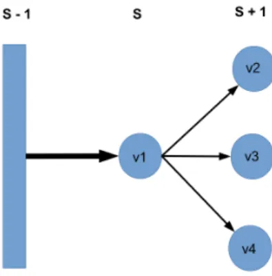
Figure 1.1: Supersteps and the message passing model
Pregel adopted the concepts proposed by the BSP model and added some extra functionality to enhance its usage for graph algorithms. In the following, I will present Pregel’s computation model, the main programming concepts and some implementation details.
Computation model
• Input/Output. Theinput of a Pregel program is a directed graph. Each vertex has a unique string id and a user-defined value. Edges are represented as tuples containing the source vertex, destination vertex and a user-defined value. The output of a computation is composed of the values written by each vertex.
• Supersteps. Supersteps are the main component of Pregel. Similar to the BSP model, a Pregel computation consists of a sequence of supersteps. During a superstep each vertex executes in parallel a user-defined function. Messages belong to a specific superstep. The messages sent in superstep s−1 will be available at their destination in superstep s. This process is shown in Figure 1.1. In supersteps−1 several messages are sent tov1. These messages are available atv1in supersteps. v1 sends a message tov2,v3andv4 in superstep s. These messages are processed byv2, v3 and v4 in superstep s+ 1. Besides performing computations, receiving, creating and sending messages, a vertex can modify its value or its outgoing edges in the course of a superstep.
• Message passing. Pregel uses the message passing model because it is sufficiently expressive and it offers a better performance than shared memory, that requires locking mechanisms.
• Termination. Termination is based on every vertex voting to halt. In superstep 0 all vertices are active. A vertex can deactivate itself by voting to halt, but it is reactivated when it receives a message. During a superstep only active vertices perform computations. The execution finishes when all vertices are inactive and there are no messages in transit that could activate a vertex.
Figure 1.2: Combiners
Figure 1.3: Aggregators
Programming concepts
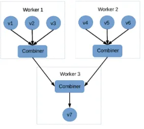
• Combiners. Besides the BSP components [1], Pregel [2] offers some extra functionality. One of the concepts that it provides are combiners. Their purpose is to reduce message traffic. For example, if the graph’s vertices store a value and the algorithm is only in-terested in computing the maximum value of the values passed through messages that arrive at vertices, then a combiner could be used. Instead of keeping all the values in the outgoing message queue and then computing the maximum at the destination, only one value is stored in the message queue. Consequently, if this value has to be sent over the network then the space for buffered messages and the traffic is minimised. An illustration of how combiners work can be seen in Figure1.2. The values of the vertices from the first and second workers are passed to the corresponding combiners. The values of these two
Figure 1.4: The order of the mechanisms employed by Pregel to achieve determinism.
combiners can be used in the next superstep to set the value of the vertexv7from Worker 3.
• Aggregators. Pregel provides through aggregators a mechanism for global coordination, monitoring and statistics computation. The difference between combiners and aggrega-tors is that combiners are doing local aggregation of outgoing/incoming messages, while aggregators are doing global aggregation of user-defined quantities. Pregel’s approach is based on local computations. Hence, aggregators enable the possibility to compute global metrics. The aggregators’ value are stored by the master. During a superstep vertices can send a value to an aggregator which applies a commutative and associative function. The result is available for all the vertices in the next superstep. Typical aggregators functions are min, max, sum, count. In order to reduce the overhead, the aggregators collect the partial values from each worker in a tree based data structure. Figure 1.3 depicts this process. The figure represents the tree structure generated by the partial aggregators. Each worker will pass its partial aggregated value to the next level of the tree until the final values will reach the master.
• Topology Mutations. Pregel employs partial ordering and handlers in order to re-solve conflicting requests to the graph’s structure. First, it performs removals, with edge removal and then vertex removal. Afterwards it executes additions requests. Vertex addi-tions have higher priority than edge addiaddi-tions. Next in order is the user defined function executed by all the active vertices. The remaining unresolved conflicts can be treated in user defined handlers. This order can be visualised in Figure1.4
Implementation
• Master. Pregel [2] is based on a Master-Worker architecture. The master coordinates the computation of the workers. At the beginning of the computation, it partitions the graph and assigns one or more partitions to each worker. Afterwards, it notifies workers to perform supersteps or save their portion of graph. Moreover, coordinates fault detection and recovery.
• Worker. Workers keep their portion of the graph in memory. During a superstep they compute the user defined function and communicate directly with each other in order to exchange messages.
local informations and the master saves the aggregators’ values. As mentioned before, the master is responsible for fault detection. It sends regular pings to the workers. If a worker does not reply it marks that worker as failed. Depending on how often the workers save their state, in the case of a failure the computation might have to repeat all the operations from some previous supersteps. If a worker does not receive a ping message from the master within a period of time it terminates.
1.2.2
Giraph
Giraph [24] is an open source implementation of Pregel released under the Apache licence. An overview of its architecture can be seen in Figure 1.5. Being part of the Hadoop ecosystem offers a number of advantages. It can easily be integrated with other Hadoop technologies and it can run on any Hadoop cluster. A Giraph computation runs as a MapReduce1 job or as a YARN2 application [22] and it uses ZooKeeper [23] for coordination. It can read/write data from/to HDFS3, HBase4, HCatalog5, Cassandra6 or Hive7 tables. Although it has the same computation model as Pregel, Giraph comes with some differences in order to make the system more reliable, flexible and scalable. In the following, I will briefly present some of these extensions.
• ZooKeeper. Giraph uses ZooKeeper [23] to perform part of the master’s attributions from Pregel. ZooKeeper is a distributed coordination system based on a shared hier-archical name space. It provides mechanisms for group membership, leader election, configurations, monitoring, barriers. Its fault tolerant services are based on an algorithm that resembles Paxos [23]. By using this coordination system, Giraph eliminates the single point of failure introduced by the master present in Pregel.
• Sharded aggregators. Unlike Pregel, where the master was in charge of aggregation, Giraph uses sharded aggregation [24]. Each aggregator is assigned to one worker that receives the partial values from the all the other workers and is responsible for performing the aggregation. Afterwards, it sends the final value to the master. Consequently, the master does not perform any computation. Moreover, the worker in charge of an aggre-gator sends the final value to all the other workers. This design decision was adopted in order to remove the possible computation and network bottlenecks generated by the master in the case of applications where aggregators are used extensively.
• Out-of-core capabilities. The main policy adopted by Pregel and Giraph is to keep everything in memory in order to avoid expensive reads and writes from the disk. Un-fortunately, in some cases the graph or the messages can exceed the cluster’s memory. Therefore, Giraph extended Pregel with out-of-core capabilities, meaning that some of the graph’s partitions and part of the messages can be saved to disk based on some user defined values and flags [24].
• Master compute. Giraph extends the Pregel model by adding a master compute function that it is called in each superstep before the vertex compute function [22]. It can be used to register, initialize aggregators or to perform centralised computations that can influence the vertex computations.
1http://hadoop.apache.org/docs/current/hadoop-mapreduce-client/hadoop-mapreduce-client-core/ MapReduceTutorial.html 2http://hadoop.apache.org/docs/current/hadoop-yarn/hadoop-yarn-site/YARN.html 3http://hadoop.apache.org/docs/r1.2.1/hdfs_design.html 4http://hbase.apache.org/ 5http://hortonworks.com/hadoop/hcatalog/ 6http://cassandra.apache.org/ 7https://hive.apache.org/
Figure 1.5: Giraph integration with the Hadoop ecosystem. Image taken from [22].
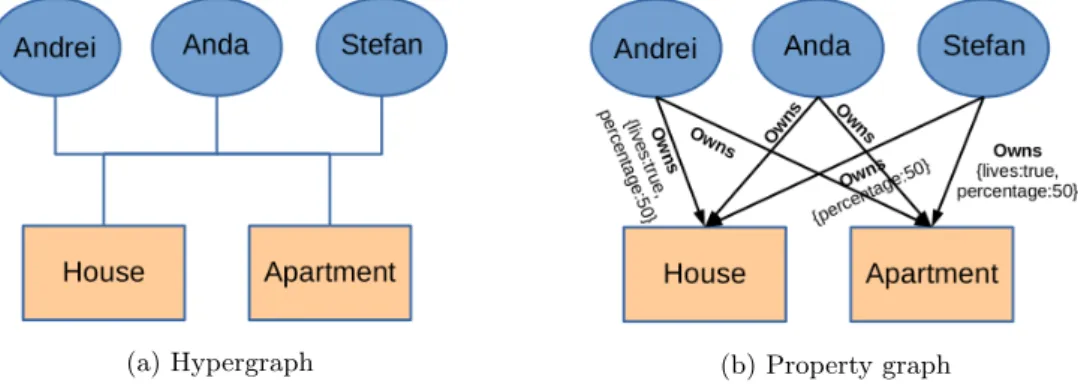
(a) Hypergraph (b) Property graph
Figure 1.6: The hypergraph and property graph corresponding to the same data
1.3
Related Work
1.3.1
Graph data models
Graph modeled data can be represented in different ways. The most common representations are property graphs, hypergraphs, and triples [10].
Property graphs
Data is represented as nodes and relationships between them. Each node contains properties (key-value pairs). Relationships are named, directed and can contain properties. This repre-sentations is common within graph databases. For example, Neo4J adopted it. We also use this representations because it is expressive and it is suitable for the Giraph model. More details about our data model can be found in the next section.
Hypergraphs
A hypergraph is a more generalised representation of a graph [10]. Unlike the previous rep-resentations where an edge can only have one start node and one end node, here an edge can connect multiple nodes. Hence, at each end of the edge there can be multiple nodes. For ex-ample, Andrei, Anda and Stefan inherited from their parents an apartment and a house. All of them own these properties. Therefore there is an edge that connects each of the childrens with the apartment and house. The graph can be seen in Figure1.6a. This graph can be easily converted to the property representation, shown in Figure1.6b. The corresponding property
graph has 6 edges instead of one, but it can hold more information than the hypergraph. It can keep what percentage does each person owe from the property, if it leaves in that property etc.
Triples
Triples are subject-object-predicate data structures that are used in the Semantic Web field. On their own triples do not provide complex informations, but their connection provides useful knowledge [10]. Hence, they are not exactly a graph structure, they can be seen as a query pattern. For example, Trinity.RDF [7] and TripleRush [6] use this representation. Both of these systems support SPAQRL queries. Usually, triples or RDF data are associated with this query language. It is not necessary that triples are represented internally in the same format. Graph databases can support SPARPQ queries while still keeping their own representation. Therefore, we could add support for SPARQL queries in the future.
1.3.2
Graph Pattern Matching Algorithms
Queries applied to a graph database or a graph system can be seen as a pattern graph. There-fore, these application are reduced to a subgraph isomorphism problem, which belongs to the NP-hard class [17]. We define an undirected labelled graph G as a triple(V, E, L), whereV
is the set of vertices,E(⊆V ×V) is the set of undirected edges and L is a labelling function which maps a vertex or an edge to a set of labels or label [17]. This formalisation can easily be extended to match the property model used by our system. We could add another functionP
that maps a vertex or an edge to a set of properties.
Given a query graph (pattern graph)Q= (V, E, L)and a data graphG= (V0, E0, L0)we define a subgraph isomorphism as being an injective functionM :V →V0 such that:
1. ∀u∈V,L(u)⊆L0(M(u))
2. ∀(ui, uj)∈E,(M(ui), M(uj))∈E0 andL(ui, uj) =L0(M(ui), M(uj))
Subgraph isomorphisms has applications in various areas such as social networks, chemistry, biology. Therefore, many algorithms that target this problem were developed. They apply different pruning rules, join orders and auxiliary neighbourhood information [17].
The first algorithm for subgraph isomorphism was introduced by Ullmann [14]. It is based on a recursive backtracking approach. It first constructs a mapping matrixM of size|V|×|V0|, where |V|is the cardinal ofV. M(i, j) = 1if it is possible thatui∼vjin some subgraph isomorphism,
where ui ∈V and vj ∈V0. They use the vertex’s degree as a criterion for matching vertices
from the pattern graph to vertices from the data graph. Compared to a brute force solution that would choose at each step a possible mapping for one vertex of the pattern, the Ullmann algorithm applies a simple pruning method. Considering two verticesui ∈ V and vj ∈V0, if
ui ∼vj then all ofui’s neighbors have to have a corresponded invj’s neighbors. IfM(i, j) = 1
and there is a neighbor ofuithat does not have a correspondent invj’s neighbors thenM(i, j)
is set to 0. The pruning is done at each step in the backtracking algorithm. The effectiveness of the pruning procedure depends on the order of the vertices. Hence, the algorithm orders the vertices such that high degree vertices ofQare first.
It is possible to adapt Ullmann’s algorithm to work with Giraph, but a pure adaptation will have to check the neighbours at each step, which will produce many messages. Furthermore, the computation will produce many supersteps. A more suitable approach is the brute force algorithm based on backtracking. One could think that each vertex keeps in memory one column from the matrix presented in Ullmann’s algorithm. The computation could traverse the pattern graph and at each stage checks if the vertex from the data graph matches the current vertex from the pattern graph. One vertex from the data graph cannot be used for more than
the matching process can be associated with a partial solution. A node is added to P(s) if it fulfils some feasibility rules. They consider two types of feasibility: syntactic and semantic. The syntactic feasibility depends only on the structure on the graphs. The semantic feasibility depends on the attributes. The number of states generated in the process is reduced by adding a set of rules, named k-look-ahead rules, which check in advance if a consistent state s has no consistent successors after k steps. Ullmann and VF2 algorithms are similar considering that both check each possible solution. The difference is made by the pruning technique. The pruning employed by the VF2 algorithm is expected to have a smaller complexity.
Giraph’s computations are vertex centric, each vertex stores only information about itself. Hence, a k-look-ahead rule would imply to send k messages or to cache locally information about the neighbours. With large data sets, storing additional information about neighbours could add significant memory overhead. Giraph’s out of core capabilities could be used to store on disk what does not fit in memory. Writing to disk or having a high number of supersteps makes the computation slow. Therefore, it is not clear if such an approach could improve the running time. In order to have a better understanding of what could be improved, for the first version of Lighthouse we wanted to see Giraph capabilities and how the system behaves with a simple approach. Consequently, this type of pruning could be adapted for Giraph and studied in the future.
The main idea behind GraphQL algorithm [18] resembles the one behind Ullmann’s [14] and VF/VF2 [15, 16] algorithms, but they extend the pruning mechanisms. They use three pruning techniques. The first technique prunes the possible mates of each node from the pattern and retrieves it efficiently through indexing. They consider the neighborhood subgraphs of each node within a distance r. It is the same pruning technique used by the VF2 algorithm. Besides what VF2 was proposing, they also consider the possibility of adding some indexes and they extend the pruning with another two techniques. The second technique prunes the overall search space by considering all nodes in the pattern simultaneously. They construct at each iteration a bipartite graph to test if a node is feasible mate of a node. The last technique applies ideas from traditional query optimization to find the right search order. GraphQL was designed for large graphs. Thus, it is more structured than the previous algorithms. It employs a graph algebra that has a select operator similar to Lighthouse’s select operator. Regarding its possible adaptation for Giraph and its efficiency, there are the same concerns expressed before for the VF2 algorithm.
SPath [19] introduces a different approach, it matches a path at each step, not a vertex. The query graph is decomposed in multiple shortest paths, which are matched against the data graph. Then, the paths are joined together in order to rebuild the query graph. They studied which pattern has the best performance for subgraph isomorphisms. They considered three different patterns: paths, trees and graphs. For each of them they evaluated two types of cost: feature selection and feature pruning cost. The feature selection cost identifies a pattern from a k-neighbourhood subgraph. The feature pruning cost matches a pattern in a k-neighborhood subgraph. For all the structures the feature selection cost is linear. The difference is made by the feature pruning cost, which is linear for paths, polynomial for trees and NP-complete for graphs. Thus, they decided to split the query graph into paths. We decided to follow this direction. A path structure can be easily computed with Giraph by matching one vertex in
each superstep and sending messages to the next possible vertex from the path. Hence, our approach follows the vertex at a time model, but adopts the paths pattern proposed by SPath. The paths generated from the query plan are joined by a HashJoin operator. More details about the paths and the operators can be found in Chapters2 and3. In the future, we could study if a different decomposition of the query pattern is more efficient.
Besides the aforementioned algorithms, there are many more algorithms that tried to improve the performance and scalability of subgraph isomorphism. A study that compared these algo-rithms by implementing them with a common framework showed that there is not an algorithm that outperforms the others on all the datasets and all the patterns [17]. Most pruning tech-niques behave better under certain circumstances. Therefore, we studied these algorithms and started with the most simple adaptation of a subgraph isomorphism algorithm for Giraph. A vertex centric distributed system adds some extra challenges to the problem. Thus, the simple approach could reveal the bottlenecks and the possible areas for improvement.
1.3.3
Graph Systems
Graph Databases
Graphs databases focus on online querying where low latency is required. Compared to rela-tional databases they have better performance for adjacency and graph traversal queries [13]. The query language used by the graph databases can be one criterion for classification. There is no standard language. Therefore, databases implement their own API or support SPARQL queries. Our decision to use Neo4j’s attached query language, Cypher [9], was determined by the expresivity of the language. Some of the most popular graph databases are: DEX1, Neo4j [8], HyperGraphDB [11], OrientDB2, Titan3. A study that compared these databases showed that there is no database that outperforms the rest for all workloads [12].
Graph Engines
Graph engines focus on offline queries that are mostly used for analytics. The Pregel model presented in Subsection 1.2.1was the source of inspiration for many graph engines. Pregel is not available to the public. Hence, the open source community provides some implementations: Giraph [24], GoldenOrb4, Phoebus5. Giraph is presented in Subsection 1.2.2. Like Giraph, GolderOrb is written in Java, uses Hadoop and it is released under an Apache licence. The difference is that it requires additional software installation6. Moreover, it does not seem to be supported anymore. Phoebus is a system written in Erlang that supports a distributed model of computation similar to MapReduce. Apart from the Pregel implementations there is also Hama7 a system that provides only BSP functionality and that it is realeased under an Apache licence.
Besides Pregel [2], there are other engines that target offline queries. One of them is Trinity [3]. This system can actually be included both at graph databases and graph engines as it supports online query processing and offline graph analytics. As Pregel, Trinity does all the computations in memory. They use a key-value store on top of a memory cloud in order to achieve the performance needed for online and offline queries. Another graph engine is Signal/Collect [4]. It is similar with Pregel in the sense that it uses a MPI model for communication. Compared
1http://www.sparsity-technologies.com/dex 2http://www.orientdb.org/ 3http://thinkaurelius.github.io/titan/ 4https://github.com/jzachr/goldenorb 5https://github.com/xslogic/phoebus 6http://blog.acaro.org/entry/google-pregel-the-rise-of-the-clones 7https://hama.apache.org/
TripleRush [6] build on top of Signal/Collect [4]. Trinity.RDF computes a SPARQL query, while STwig’s query pattern is a labelled graph. The main concept used by the computation of the two algorithms is the same. One difference is the pattern used to decompose the query. STwig splits the graph into trees of level two, called STwigs. Trinity.RDF decomposes the query in RDF patterns. The root node of tree pattern can have more children. In Trinity.RDF the pattern has one entity at each side, a root with one child. Thus, the pattern employed by STwig is more complex. Another difference is the type of index used. STwig uses a local index to find the vertices with a certain label. Each machine keeps track for each label which local vertices have that label. Trinity.RDF used some indexes for the predicates. It keeps a local predicate index and a global predicate index. The local index is used by vertices to find quickly if they have a certain predicate, while the global one stores which subjects and objects refer that predicate. It stores a list of ids for each machine, where an id points to the list of subjects/objects that are stored on that machine and are related to the predicate. TripleRush [6] has the same purpose as Trinity.RDF to answer a SPARQL query and it is based on a index graph. In the following I will refer to STwig because its approach matches our goals.
As mentioned before, STwig split the query into tree structures of level two. The authors chose a small pattern in order to avoid additional indexes. The downside of this solution is that it produces a large number of joins and intermediary results. Hence, the STwig decomposition and order selection have a big impact on the performance. Their approach can be adapted for Giraph. The label frequencies could be computed in the first superstep of the computation using an Aggregator. Another possibility is to read them from a statics file, similar to our current approach. Afterwards, the STwigs can be generated. We could divide the computation in phases, where each phase computes partial result for a STwig. There are two possible ways to match a STwig. One could start from the root or from the children of the root. Starting from the root would produce three supersteps for each STwig. In the first superstep of a phase each vertex checks if its label corresponds with the root label of the phase pattern. If the condition is true then it sends a message to all of its neighbours with its id. There are two possible optimisations. Firstly, if the number of outgoing edges is less than the number of elements from the pattern then the computation abandons that partial solution. Secondly, the vertices could store the labels of the neighbours. The second time a vertex is considered as root for a STwig, it does not have to generate additional computation for finding the labels. Therefore, the pattern could be matched in one superstep. If the second optimisations is not employed, then in the second superstep the vertices that received a message send back their id and their label. In the third superstep the root vertex checks the labels of the children and generates the possible solutions. Starting from the children of the root would produce two supersteps. In the first superstep the children would be scanned and would send a message to the root. In the second superstep the root would generate all the possible solutions. The performance of these solutions depends on the topology of the data and pattern graph. Based on the statistics, one could use a combination of these approaches. The algorithm proposed by STwig computes STwigs based on a order that prunes the number of solutions. A variation of the algorithm that could be investigates is to compute all STwigs in parallel and just merge them sequentially. The disadvantage is that the partial solutions might not fit into memory. The benefit of this approach is that the computation would have less supersteps and the overall running time might be smaller than in the previous case.
1.4
Research Questions
1. Could a NP complete problem benefit from the distributed environment? Would it help to scale? How much can it scale?
2. What are the different options of mapping Cypher into Giraph? Which are the advantages and disadvantages of each option?
3. Could all the functionality from Cypher be translated into Giraph? (a) Would it be more scalable than Neo4j?
(b) How much slower would it be?
(c) Would it be scalable for all the queries?
(d) Would there be operators/functions that could be considered bottlenecks for the system? Which are those operators/functions? Why they cannot be expressed effi-ciently with Giraph?
Lighthouse architecture and algebra. In the last section I describe the types of query plans used by Lighthouse.
2.1
Data Model
We use the property graph model to represent the data. Giraph’s [24] API allows users to define their representation of vertices and edges values making this model the perfect candidate for our underlying system. Each edge in Giraph has one target vertex and one destination vertex, consequently the hypergraph data model is less practical for this configuration. Triples are less expressive than the property graph and less flexible when it comes to adding new data. Our data model is based on properties and labels, where:
• Properties are key value pairs, the key is conceptually a String1, while the values can be any basic type.
• Labelsare Strings.
Vertices and edges are the elements that store information:
• Verticescan have one or multiple labels and zero or more properties. • Edgeshave one label and zero or more properties.
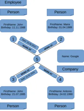
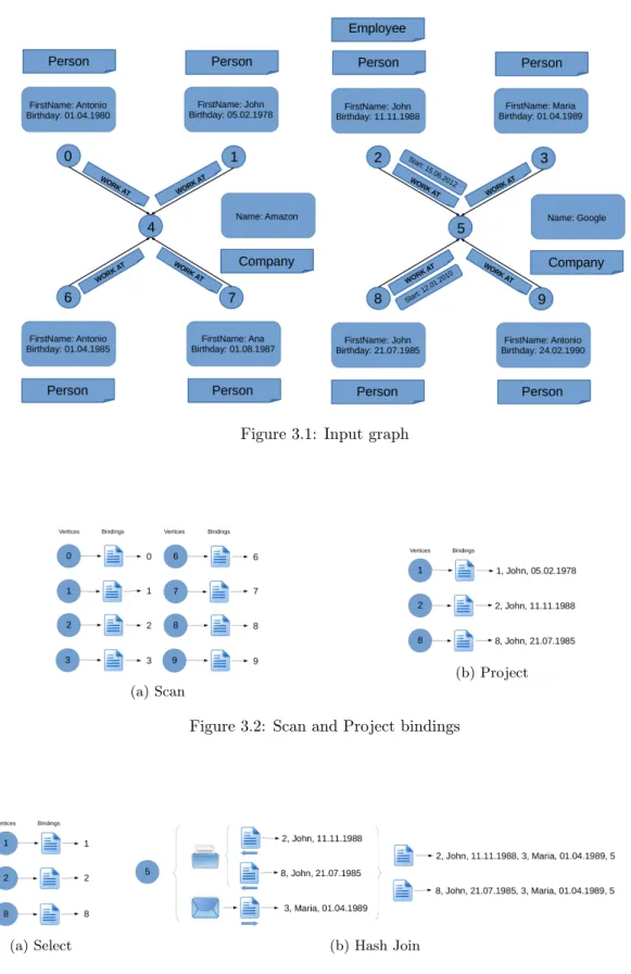
An example can be seen in Figure 2.1. There are 5 vertices and 4 edges. v2, v3 and v4 are labelled withPerson. v1has two labelsPerson andEmployee. v5is labelled with Company. v1,
v2,v3 and v4 have two vertex properties: FirstName and Birthday. All the edges are labelled withWORK_AT and two of them (v1,v5), (v3,v5), have one property: start.
2.2
Query language
Our goal is to express with Lighthouse part of the functionality offered by the Cypher query language [9]. We are currently focusing on the read queries. The structure of the queries that we support can be seen in Table2.1. We currently do not provideORDER BY,LIMIT, SKIP
1In the implementation we convert Strings to numbers in order to increase performance, but they can be
thought of as being Strings.
Figure 2.1: Example of a graph
Cypher Read Query Structure Lighthouse Query Structure [MATCH WHERE]
[ OPTIONAL MATCH WHERE]
[WITH [ORDER BY] [ SKIP ] [ LIMIT ] ] [RETURN [ORDER BY] [ SKIP ] [ LIMIT ] ]
[MATCH WHERE] [WITH]
[RETURN] Table 2.1: Cypher/Lighthouse Query Structure
capabilities. The expressions in theWHERE clause can use the operators shown in Table2.2. Unlike Cypher, we do not offer collection and regular expression operators.
An example of a Cypher query supported by Lighthouse is depicted in Cypher Query2.1. The query looks for people named Antonio that use the browser Chrome and work at a company that is located in the same country as the university he attended.
2.3
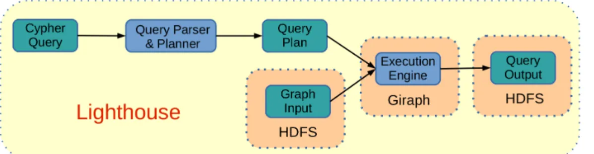
Lighthouse Architecture
Figure 2.2 presents an overview of Lighthouse’s architecture. Our system receives as input a Cypher query [9] and a graph. The cypher query is parsed and transformed into a internal representation of the query. Afterwards, the query optimiser chooses the best query plan. This
Operators Mathematical +,−,∗,∧,%, /
Comparison =, <>, <, >, <=, >=
Boolean AND, OR, XOR, NOT
String +
Figure 2.2: Lighthouse architecture
plan and the graph input are passed to the engine. The engine reads the graph and processes the query. The result is written to HDFS. In the following, I will briefly present each of these components. More details can be found throughout this thesis.
• Cypher Query. As mentioned before, our system accepts as input queries expressed in the Cypher query language. More information about the subset of the Cypher queries supported by Lighthouse can be found in Section2.2.
• Query Parser & Planner. The Cypher query is parsed and a query graph is created out of it. Afterwards, the statistics file, which contains information about the input graph, is read. These statistics are used for approximating the cost of an operation. In order to produce the best physical plan a branch-and-bound approach is used. It first chooses the cheapest solution and then prunes other solutions if the cost is above the minimum found. At each step all possible operations and their costs are checked.
• Execution engine. The execution engine leverages Apache Giraph [24]. An overview of this system can be found in Subsection1.2.2. The algebra used by the engine is presented in Section2.4. More details about the implementation can be found in Chapter3. • Input Graph. The input graphs were generated with the LDBC DATAGEN – A realistic
social network data generator1 which produces data simulating the activity of a social network site during a period of time. The data follows the same distribution as the one from a real social network and it uses information from DBPedia2.
• Query Output. At the end of the computation each worker writes its results of the queries to HDFS.
1http://ldbcouncil.org/blog/datagen-data-generation-social-network-benchmark 2http://dbpedia.org/
Specification 2.1Basic Types used by the Lighthouse Algebra
1: Constant⇒[< T ext, P roperty >]
2: P roperty⇒[key:T ext, value:< T ext, LongW ritable >]
3: P roperties⇒ {p|\p← {property:P roperty}, p.key is unique}
4: Expression⇒+(e1:Expression, e2:Expression)| −(e1:Expression, e2:Expression)| ∗(e1:Expression, e2:Expression)| /(e1:Expression, e2:Expression)| ∧(e1:Expression, e2:Expression)| AN D(e1:Expression, e2:Expression)| OR(e1:Expression, e2:Expression)|
XOR(e1:Expression, e2:Expression)|
N OT(e:Expression)| = (e1:Expression, e2:Expression)| >(e1:Expression, e2:Expression)| <(e1:Expression, e2:Expression)| ≤(e1:Expression, e2:Expression)| ≥(e1:Expression, e2:Expression)| property:P roperty | text:T ext| number:int
5: ColumnList⇒ {||expression:Expression||}
6: QueryP ath⇒ {||< Scan, Select, P roject, M ove, StepJ oin >||} 7: QueryP lan⇒ {QueryP lan}
2.4
Lighthouse Algebra
At the beginning of this section are presented the types used by the algebra and a formalisation of Giraph and Lighthouse computations. Afterwards, I specify the Lighthouse algebra opera-tors. We divide them in local and global operaopera-tors.
Since we wanted to have a clear picture of Giraph capabilities, our approach was to materialize all of the operators from the algebra. Therefore, we were able to see the properties of each operators and test if they potentially could be a bottleneck. Another benefit of this decision is that the system can easily adapt based on the performance of an operator. After a part of the query plan is executed, there are some reliable information about the output, consequently the query plan can be modified accordingly. Further extensions or changes of this algebra can be found in Chapter6.
The types specification follows the comprehension syntax [25]. An overview of the basic types used in the Lighthouse Algebra can be seen in Specification2.1. These types are used as param-eters for the operators or by the main types to express different parts from the data model. The components of the main types: Edge, Vertex, Message are presented in Specification2.2. In the aforementioned section we also define Lighthouse’s central data structure: the MessageBinding. We primarily refer to it throughout the thesis as the binding. It is the main component of the Messages and it stores the partial results computed during the execution of a query. Conceptu-ally, it can be seen as a table row from a tradition database. Specification2.4presents a higher level overview of a giraph computation. The core of the Lighthouse algorithm is described in Specification2.3. This is the computation performed by each vertex in each superstep.
8: HashJ oinM ap⇒ {entry|\entry← {id:int,
hashJ oinBindings:HashJ oinBindings}, entry.id is unique}
9: V ertexV alue⇒[labels:{T ext}, properties:P roperties, hashJ oinM ap:HashJ oinM ap]
10: V ertex⇒[id:V ertexId, value:V ertexV alue, edges:{Edge}, active:Boolean]
11: V ertices⇒ {V ertex}
Specification 2.3Lighthouse Computation
1: Computation ⇒[ context : Context [queryPlan : QueryPlan], 2: procedurecompute(vertex, messages)
3: for allmessageinmessagesdo
4: context.getQueryItem(message.path, message.step).compute(this, vertex, message)
5: end for
6: vertex.voteT oHalt()
7: end procedure]
2.4.1
Local operators
This type of operators perform computations based on the local information of the vertices. They do not increase the number of supersteps. Lighthouse’s algebra has four local operators: Scan, Select, Project, HashJoin. In the following, I will present their specification.
Scan
Scan operator is equivalent to a broadcast. Currently, it is only used as the first operator of a query plan. Its purpose is to reduce the number of starting vertices by applying an initial filter. It can filter based on the label of the vertices or on a property of a vertex. Its specification can be seen in Specification2.5.
Select
The Select operator is used to filter potential solutions that do not meet a criterion, which is expressed as a boolean expression. A description of its outcome is presented in Specification2.6.
Project
The Project operator is used to retrieve information stored by the vertex other than the vertex id. For example, it can retrieve a subset of the columns from the initial binding, add to the binding vertices’s property values or to add to the binding expression values. Its specification can be seen in Specification2.7.
Specification 2.4Giraph Computation
1: GiraphComputation⇒[ context : Context [queryPlan : QueryPlan],
2: procedurecompute(vertices)
3: superstep←0
4: whilecountActiveV ertices()>0 ormessagesInT ransit() ==true do
5: for allvertexin activeV erticesdo
6: messages←getM essagesOf T arget(vertex.id)
7: computation.compute(vertex, messages)
8: end for
9: superstep←superstep+ 1
10: end while
11: end procedure]
Specification 2.5Scan Operator
1: Scan⇒[ constant:Constant,
2: procedurecompute(computation, vertex, message)
3: if constant.eval(null, vertex.value, null) ==true then
4: message.binding.add(vertex.id)
5: message.step←message.step+ 1
6: nextOperator←computation.context.getQueryItem(message.path, message.step)
7: nextOperator.compute(computation, vertex, message)
8: end if
9: end procedure]
Hash Join
At a higher level the HashJoin operator can be seen as the operator that joins two pattern graphs. It merges two branches of the query tree. The combined messages from the left and right paths will follow the left path of the HashJoin node. An overview of its actions can be seen in Specification2.8. It is not recommended to be used in the query plan if many solutions are produced by both sides of the operator, since it will keep in the vertex memory the partial solutions.
2.4.2
Global operators
Global operators increase the number of supersteps because they involve sending messages. Basically, the number of global operators determines the number of supersteps. Our algebra has two global operators: StepJoin and Move.
Move
The Move operator moves the computation from the current vertex to a vertex that was previ-ously visited and its id is in the binding table. This operator was introduced in order to be able to retrieve at a later stage information that is no longer local. We can access the local informa-tion of a previous vertex or its edges. If the query graph is an Eulerian Graph then the Move operator is not necessarily needed, unless we want to access the properties of a vertex after the computation has already passed that vertex. Its specification can be seen in Specification2.9.
Specification 2.7Project Operator
1: Project⇒[ columnList : ColumnList,
2: procedurecompute(computation, vertex, message)
3: for allcolumnin columnListdo
4: message.binding.add(column.compute(message.binding, vertex.value))
5: end for
6: message.step←message.step+ 1
7: nextOperator←computation.context.getQueryItem(message.path, message.step)
8: nextOperator.compute(computation, vertex, message)
9: end procedure]
Step Join
The StepJoin operator filters the solutions based on the validity of an expression applied on the edges of a vertex. If an edge satisfies the StepJoin condition then the computation is moved to the target vertex of that edge. An overview of its actions can be seen in Specification2.10.
2.5
Query Plans
Our system supports two types of query plans: left deep and bushy query plans. The type of the plan is determined by the presence of the HashJoin operator.
2.5.1
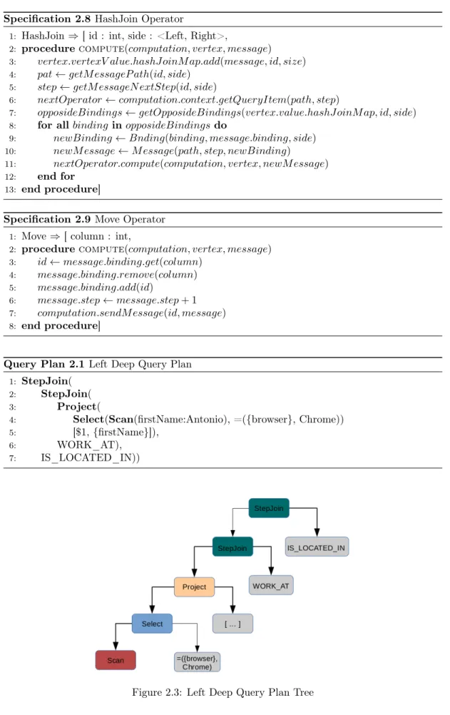
Left Deep Query Plans
In left-deep trees, the right-hand-side input for each operator is their parameter, not another operator. In Query Plan 2.1 is depicted a possible query plan of the Cypher Query2.2. An overview of the query plan tree can be seen in Figure2.3. The query looks for the countries where are located companies that have as employees people named Antonio that use the browser Chrome. The Lighthouse query plan starts by scanning people named Antonio. Then it filters the partial solutions based on whether they use the browser Chrome. Afterwards, a Project operator is used in order to add to the solution the first name of the person. The last two op-erators are two StepJoin opop-erators that make the connection with the corresponding Company and Country vertices.
Specification 2.8HashJoin Operator
1: HashJoin ⇒[ id : int, side : <Left, Right>,
2: procedurecompute(computation, vertex, message)
3: vertex.vertexV alue.hashJ oinM ap.add(message, id, size)
4: pat←getM essageP ath(id, side)
5: step←getM essageN extStep(id, side)
6: nextOperator←computation.context.getQueryItem(path, step)
7: opposideBindings←getOpposideBindings(vertex.value.hashJ oinM ap, id, side)
8: for allbindingin opposideBindingsdo
9: newBinding←Bnding(binding, message.binding, side)
10: newM essage←M essage(path, step, newBinding)
11: nextOperator.compute(computation, vertex, newM essage)
12: end for
13: end procedure]
Specification 2.9Move Operator
1: Move⇒[ column : int,
2: procedurecompute(computation, vertex, message)
3: id←message.binding.get(column)
4: message.binding.remove(column) 5: message.binding.add(id)
6: message.step←message.step+ 1
7: computation.sendM essage(id, message)
8: end procedure]
Query Plan 2.1 Left Deep Query Plan
1: StepJoin(
2: StepJoin(
3: Project(
4: Select(Scan(firstName:Antonio), =({browser}, Chrome))
5: [$1,{firstName}]),
6: WORK_AT),
7: IS_LOCATED_IN))
10: end for
11: end procedure]
Cypher Query 2.2
MATCH(person:Person{firstName:"Antonio"}) - [:WORK_AT] -> (company) - [:IS_LOCATED_IN] -> (country)
WHEREperson.browser ={"Chrome"}
RETURNperson.id, person.firstName, company.id, country.id
2.5.2
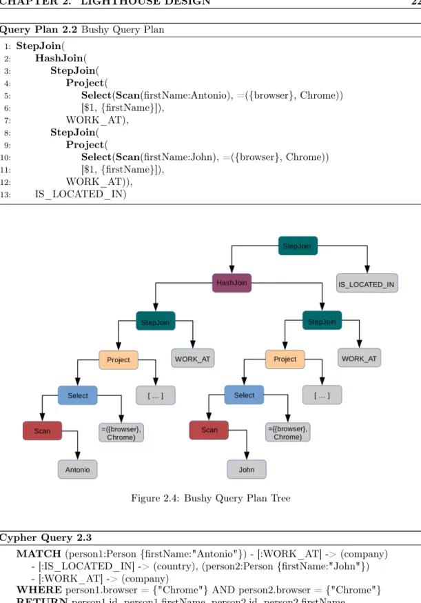
Bushy Query Plans
Bushy trees are generated by the HashJoin operator, whose right hand side is a sequence of operators, not just a parameter. In QueryPlan 2.2 is presented a possible query plan of the Cypher Query2.3. A visualisation of the query plan tree can be seen in Figure2.4. The query looks for people named Antonio and John that use the browser Chrome and work at the same company. The query is also interested in the country where the company is located. It has two main branches. The first one scans people named Antonio. It applies a Select to filter the persons that do not use the browser Chrome. Then it does a StepJoin to go to the Company labelled vertices. The second branch does the same operations, the only difference is that it scans for people named John. These two branches are merged by the HashJoin operator. The last operator is a StepJoin towards Country labelled vertices.
This type of query plan can be efficient if there are a few number of solution coming from both sides of the HashJoin operator. In some cases it can be the only way to unify two pattern graphs. In other situations it can be provide a more cost efficient plan. Lets assume that there are edges connecting companies and employees and there are many companies and all of them have a significant number of employees. In this case a possible plan could scan the companies, perform the computations for one of the branches, then move the computation back to the company and perform the computations for the second branch. It is clear that the busy plan is more efficient as the two branches are computed in parallel, consequently there are fewer number of supersteps. Moreover, if the names of the people are uniformly distributed there are a just few people named Antonio and John.
Query Plan 2.2 Bushy Query Plan
1: StepJoin(
2: HashJoin(
3: StepJoin(
4: Project(
5: Select(Scan(firstName:Antonio), =({browser}, Chrome))
6: [$1,{firstName}]),
7: WORK_AT),
8: StepJoin(
9: Project(
10: Select(Scan(firstName:John), =({browser}, Chrome))
11: [$1,{firstName}]),
12: WORK_AT)),
13: IS_LOCATED_IN)
Figure 2.4: Bushy Query Plan Tree
Cypher Query 2.3
MATCH(person1:Person{firstName:"Antonio"}) - [:WORK_AT] -> (company) - [:IS_LOCATED_IN] -> (country), (person2:Person{firstName:"John"}) - [:WORK_AT] -> (company)
WHEREperson1.browser ={"Chrome"} AND person2.browser ={"Chrome"}
RETURNperson1.id, person1.firstName, person2.id, person2.firstName, company.id, country.id
implementation details of the operators and show illustrations of their actions. In the last section, I shown on an example the computations done by Lighthouse when executing a query plan.
3.1
The Lexer and Parser
The Execution Engine receives the query plan as a string. Each worker parses this input and constructs the query plan tree. This transition is done using CUP1 parser and JFLEX2lexer.
3.2
Query Paths
We split the query plan tree into multiple paths. For left deep plans we only generate one path. For busy query plans the number of paths is determined by the number of HashJoin operators. Each HashJoin operator joins the paths that come from the left and right hand side. The paths are computed in parallel and after the join the messages will follow the left path, as the right path will always finish at the HashJoin operator. For example, from the query plan tree depicted in Figure2.4the system generates two paths:
1. The first path that is generated can be seen in Query Path3.1. It includes all the elements from the left side of the tree, similar to a left deep plan.
2. The second path that is generated from the query tree can be visualised in Query Path3.2. The path is the right hand side of the HashJoin operator. It stops at this operator since after the merge the left path is continued.
Messages keep track of the path they follow and of the step from the path that has to be executed. Therefore, each message follows its path independently.
1http://www2.cs.tum.edu/projects/cup/index.php 2http://jflex.de/
Query Path 3.1Left Side
1: StepJoin(
2: HashJoin(
3: StepJoin(
4: Project(
5: Select(Scan(firstName:Antonio), =({browser}, Chrome))
6: [$1,{firstName}]),
7: WORK_AT),
8: IS_LOCATED_IN)
Query Path 3.2Right Side
1: HashJoin(
2: StepJoin(
3: Project(
4: Select(Scan(firstName:John), =({browser}, Chrome))
5: [$1,{firstName}]),
6: WORK_AT)),
3.3
Binding Table
The bindings are the core data structure of Lighthouse. They store intermediate results and were inspired by traditional databases tables. We started from this concept and adapted it to our distributed, vertex centric environment. Giraph provides two storing units: vertices and edges and a message passing model for communication. Therefore, one option to construct the solution is to embed the binding table into messages. During a superstep vertices receive messages that are further passed to the corresponding operators from the query plan. These operators process the message based on the vertex and binding table information. Hence, in the binding table are added all the information that are needed either to prune the solution at a later stage or in the final result. It is a list of vertex ids, property values and expression results. Bindings are the horizontal partition of a table, that are constructed sequentially based on the local information of the vertices. Conceptually, during a superstep the columns of a row are “updated”.
3.4
Operators
In the following, I will present more details about the implementation of the operators and I will describe their execution on some example applied on the input graph depicted in Figure3.1.
3.4.1
Local operators
Local operators do computation based on the information stored by the vertices. Afterwards, they pass the computation to the next operator from the path or store the solution in case it is the last operator from the path.
Scan
As mentioned before, Scan operator is the first operator from a query plan. For example, if the query plan starts with a Scan(Person), there will be 8 vertices that will create a binding as
Figure 3.1: Input graph
(a) Scan
(b) Project
Figure 3.2: Scan and Project bindings
(a) Select (b) Hash Join
there are 8 vertices labelled with Person. These bindings contain the id of vertex that created them. They can be seen in Figure3.2a.
Select
The Select operator has the purpose to trim down the number of solutions based on some boolean expression. Lets assume that we are not interested in all the Persons. We want to know something about persons whose first name is John. The query plan could have after the previous Scan operator a Select(=({firstName}, John)). All the vertices that have a binding apply this boolean expression on their local information. There are only three verticesv1, v2, v8 that satisfy the condition. The remaining bindings are shown in Figure3.3a.
Project
The previous operators were only adding to the bindings vertices ids or filter the solution. In order to retrieve the information stored by the vertices the project operator has to be used. For example, we would like to have in the solution the first name and the birthday of the people. The query plan could apply a Project([$1,{firstName},{birthday}]) after the Select operator. The first element from the column list denotes that we keep the first element from the binding. The second and third elements add to the binding the value of the properties ,{firstName},{birthday}. The outcome of this operator can be seen in Figure 3.2b.
Hash Join
The implementation of the HashJoin operator follows the ideas of the Pipeling hash-join pre-sented by Wilschut et al. [21]. The join process consists of only one phase, unlike other types of implementation. One advantage of this approach is that it produces output faster. Moreover, it is more appropriate for the pipeline approach presented in the Chapter 6. Other types of implementation would imply adding an additional superstep to the computation.
The HashJoin operator has an important role, to merge paths, but is also the most costly op-erator from a memory point of view. It is the only opop-erator that uses additional memory. The other operators perform computations on the messages that arrive at a vertex in a superstep, without storing any additional information. On the contrary, for each HashJoin operator each vertex stores a table containing the bindings that came from the left and right side of the tree. These tables are kept in memory. In order to increase the scale of the system the out of core capabilities provided by Giraph could be used. To illustrate HashJoin’s actions lets assume that we are interested in people named John and Maria that work at the same company. The query plan could use a HashJoin operator to merge the path that scans for people named Maria that work at a company with the one that scans for people named John. An overview of the process is shown in Figure3.3b. Vertex5has stored in the table associated with this HashJoin operator two bindings that came from the left side. When a message with a binding from the right side arrives at this vertex, it is merged with the bindings from the table. The operator will produce two bindings containing the binding from the left side first and then the binding from the right side. At the end of the binding it is added the id of the current vertex, namely 5.
3.4.2
Global operators
The global operators establish the communication between vertices. They are the only operators that call the sendMessage method provided by the computation class. Consequently, they produce network traffic and increase the number of superstep.
Step Join
StepJoin operator adds to the path a new vertex based on a label or edge expression. For exam-ple, we consider that the query plan from the Project operator contains aStepJoin (WORK_-AT) after the Project operator. Vertices1,2, and 8 will check which of their outgoing edges satisfy this condition. Each of these vertices has one edge that satisfy the condition of the operator: (v1, v4), (v2, v5), (v8, v5). They add in the binding table the id of the target vertex and send the message to this target. A visualisation of the process can be seen in Figure3.4a.
Move
The Move operator can be used to access information that is no longer local. Let’s assume that after the previous StepJoin the query plan has aMove($1). This means that the computation goes back to the vertex whose id is the first in the binding. Vertex5, has two bindings, it moves the ids situated on the first position at the end of the bindings as it can be seen in Figure3.4b. We always keep on the last position of the binding the target id of the future message. The first binding from vertex5will be send to vertex2, while the second binding will be send to vertex
8. The same computations are done by vertex 4 which sends a message to vertex 1. These messages will be available at their destination in the next superstep.
3.5
Lighthouse Example
In the following, I will present the computations done by Lighthouse when executing the Cypher Query3.1with the Query Plan3.1. The query looks for two people named Antonio and John who work at the same company and Antonio is two years younger than John. The computation produces from this query plan two query paths: QueryPath 3.3 and QueryPath 3.4. The solutions will be produced in four supersteps:
• In superstep 0, each path does a Scan and a StepJoin. The bindings produced by each path are presented in Table 3.1. They contain the id of the current vertex and the id of the target vertex. Only the vertices that store the information for a person named Antonio or John created a binding. Each of these vertices has only one edge labelled with “WORK_AT”. These bindings are sent to the target vertex.
• In superstep 1, vertices receive the messages sent in the previous superstep. The bindings present at each vertex are shown in Table 3.2. These bindings are combined by the HashJoin operator. The result can be seen in Table 3.3. Afterwards, the first Move operator is applied, which moves the computation back to the first visited vertex from Path 0. The first column is moved to the last position in the binding as it can be seen
in Table 3.4. The bindings are packed into messages and sent to their target, which is vertex id from the last column.
• In superstep 2, the first Project operator is applied in order to get the birth year of the persons named Antonio. The bindings are presented in Table3.5. Afterwards, the second Move operator computed. It moves back the computation to the first vertex from the second path. The structure of the bindings before the messages are sent can be seen in Table3.6.
• In superstep 3, the second project operator retrieves the birth year of the second person. The bindings are shown in Table 3.7. At the end a Select operator, that checks if the difference between the birth year of two persons is 2, trims down the solutions. As it can be seen in Table3.8 there are only two results for this query.
Query Plan 3.1 Example of query plan
1: Select( 2: Project( 3: Move( 4: Project( 5: Move( 6: HashJoin(
7: StepJoin(Scan(firstName:Antonio), WORK_AT),
8: StepJoin(Scan(firstName:John), WORK_AT)),
9: [$1]),
10: [$1,$2,$3,year({Birthday}])),
11: [$1]),
12: [$1,$2,$3,$4,year({Birthday}),−($3, year({Birthday}))]),
13: = ($6,2))
Query Path 3.3Query Path 0 of QueryPlan 3.1
1: Select( 2: Project( 3: Move( 4: Project( 5: Move( 6: HashJoin(
7: StepJoin(Scan(firstName:Antonio), WORK_AT),
8: [$1]),
9: [$1,$2,$3,year({Birthday}])),
10: [$1]),
11: [$1,$2,$3,$4,year({Birthday}),−($3, year({Birthday}))]),
12: = ($6,2))
Query Path 3.4Query Path 1 of QueryPlan 3.1
1: HashJoin(
Vertex $1 $2 0 0 4 6 6 4 9 9 5 Vertex $1 $2 1 1 4 2 2 5 8 8 5 Table 3.1: Superstep 0 Path 0 Binding Vertex $1 $2 4 0 4 4 6 4 5 9 5 Path 1 Binding Vertex $1 $2 4 1 4 5 2 5 5 8 5
Table 3.2: Superstep 1 before the HashJoin operator is applied
Binding Vertex $1 $2 $3 4 0 1 4 4 6 1 4 5 9 2 5 5 9 8 5
Table 3.3: Superstep 1 after the HashJoin operator is applied Binding Vertex $1 $2 $3 4 1 4 0 4 1 4 6 5 2 5 9 5 8 5 9
Table 3.4: Superstep 1 before the Move op-erator sends the messages
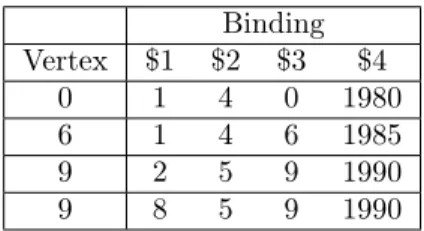
Binding Vertex $1 $2 $3 $4 0 1 4 0 1980 6 1 4 6 1985 9 2 5 9 1990 9 8 5 9 1990
Table 3.5: Superstep 2 after the Project op-erator is applied Binding Vertex $1 $2 $3 $4 0 4 0 1980 1 6 4 6 1985 1 9 5 9 1990 2 9 5 9 1990 8
Table 3.6: Superstep 2 before the Move op-erator sends the messages
Binding Vertex $1 $2 $3 $4 $5 $6 1 4 0 1980 1 1978 2 1 4 6 1985 1 1978 7 2 5 9 1990 2 1988 2 8 5 9 1990 8 1985 5
Table 3.7: Superstep 3 after the Project op-erator is applied
Binding
Vertex $1 $2 $3 $4 $5 $6
1 4 0 1980 1 1978 2
2 5 9 1990 2 1988 2
Table 3.8: Superstep 3 after the Select oper-ator is applied
They showed that our system is network bound. The last section targets this issue by informing of a possible solution.
4.1
Setup
For the experiments we used Giraph 1.1.0. Each worker had assigned 16G of Heap. In the following are presented more information about the data set and cluster.
4.1.1
Data set
For Lighthouse’s evaluation we used three data sets that simulate the activity of a social network. The number of entities from the main types used in our queries are shown in Table 4.1. We consider the central point of our data set the persons. Therefore, I will refer to a data set with the number of the person from that data set. 10K is the data set that has 10000 persons.
4.1.2
Cluster
We ran the experiments on the Surf Sara Hadoop Hathi cluster1. The cluster has 90 data/com-pute nodes with 720 CPU-cores2.
1https://surfsara.nl/systems/hadoop/hathi 2https://surfsara.nl/systems/hadoop/description
DataSet #P erson #Comment #P ost #T ag
10K 10.000 896.995 95.058 12.858
50K 50.000 6.428.749 679.267 64.734
100K 100.000 14.921.364 1.576.380 129.906 Table 4.1: Data set entities
4.2
Scalability
We tested the scalability of our system in three directions: worker, thread and size scalability. The results are presented in the following.
4.2.1
Worker scalability
Our first experiment varied the number of workers in order to see if we can get a time im-provement. For this evaluation we used the Cypher Query 4.1, the query plan presented in Query Plan 4.1 and the 10K data set. The query looks for comments that have as author a male that liked a post for which the browser used was Chrome. The results can be seen in Figure 4.1. In the chart we can see the time for all the supersteps and the total time. There is no time improvement when increasing the number of workers. Consequently, our system is network bound. Increasing the number of workers can actually lead to a time increase because there will be more communication. We verified this hypothesis by running the same experiment with messages that had double size. The running time was almost double compared with the previous case. Thus, most of the time is spent on communication.
Cypher Query 4.1
MATCH(comment:Comment)-[:has_creator]->(person:Person)-[:likes]->(post:Post)
WHEREpost.browserUsed ={"Chrome"}AND person.gender ={"male"}
RETURNcomment.id, person.id, friend.firstName, friend.creationDate, friend.gender, post.content, post.creationDate;
Query Plan 4.1 Plan used for the worker/thread scalability evaluation
1: Project(
2: Select(
3: StepJoin( 4: Project(
5: Select(,
6: StepJoin(Scan(Comment), has_creator),
7: = ({gender}, male))
8: [$1,$2,{f irstN ame},{creationDate},{gender}]),
9: likes),
10: = ({browser}, Chrome)),
Figure 4.1: Worker scalability
4.2.2
Thread scalability
In order to prove that Lighthouse is network bound we also tried varying the number of threads. For the experiment we used Query Plan4.1, 64 workers and the 10K data set. The results are depicted in Figure 4.2. Since the system is not CPU bound and most of the time is spent on communication, we can see that there is no time improvement.
Figure 4.2: Thread scalability
4.2.3
Size scalability
Giraph scales when the size of the dataset is increased. Consequently, one of our expectations was that Lighthouse will scale from the size perspective. For the experiment we varied the number of persons from the dataset and kept the number of workers constant. We used the Cypher Query4.2with the Query Plan 4.2, 64 workers and the data sets from Table4.1. The query looks for persons that have a friend that have a friend named Jacques, hence a two step relation. The results are depicted in Figure4.3. It can be seen that the running time increases
proportional with the size of the data set. Therefore, our system does scale from the size per-spective.
This experiment also proofs that a NP complete problem can benefit from a distributed en-vironment. It is highly unlikely that a single machine could query data sets of more than 16 million items. We have resumed to three datasets, but we are confident that for this query and the same setup the system can scale even more. Queries that scan all the comments and pass their information might need a higher number of machines or heap memory. The scalability of a query is influenced by the resources allocated for the job, the number of messages and their size.
Query Plan 4.2 Plan used in the size scalability evaluation
1: Project(
2: Select(
3: StepJoin(
4: StepJoin(Scan(Person), has_knows),
5: knows),
6: = ({f irstN ame}, J acques)),
7: [$1,$2,{f irstN ame},{creationDate}, {gender},{browserU sed},{locationIP}])
Cypher Query 4.2
MATCH(person1:Person)-[:knows]->(person2:Person)-[:knows]->(friend:Person)
WHEREfriend.firstName ={"Jacques"}
RETURNperson1.id, person2.id, friend.firstName, friend.creationDate, friend.gender, friend.browserUsed, friend.locationIP;
Figure 4.3: Size scalability
4.3
Late/Early projection
Since our system is network bound one way to improve the running time is to minimise the number of bytes sent through the network. One method to reduce the communication is to use late projection instead of an early projection. In order to test this hypothesis we used Cypher