Context dependent random walk graph kernels and tree pattern graph matching kernels with applications to action recognition

BIROn - Birkbeck Institutional Research Online

Hu, W. and Wu, B. and Wang, P. and Yuan, C. and Li, Y. and Maybank,

Stephen (2018) Context-dependent random walk graph kernels and tree

pattern graph matching kernels with applications to action recognition. IEEE

Transactions on Image Processing , ISSN 1057-7149. (In Press)

Downloaded from:

Usage Guidelines:

Please refer to usage guidelines at or alternatively

Context-Dependent Random Walk Graph Kernels and Tree Pattern

Graph Matching Kernels with Applications to Action Recognition

Weiming Hu, Baoxin Wu, Pei Wang, and Chunfeng Yuan

(CAS Center for Excellence in Brain Science and Intelligence Technology, National Laboratory of Pattern Recognition, Institute of Automation, Chinese Academy of Sciences; University of Chinese Academy of Sciences, Beijing 100190)

{wmhu, bxwu, pei.wang, cfyuan }@nlpr.ia.ac.cn

Yangxi Li

(National Computer network Emergency Response technical Team/Coordination Center of China, Beijing 100055) [email protected]

Stephen Maybank

(Department of Computer Science and Information Systems, Birkbeck College, Malet Street, London WC1E 7HX) [email protected]

Abstract: Graphs are effective tools for modeling complex data. Setting out from two basic substructures, random walks and trees, we propose a new family of context-dependent random walk graph kernels and a new family of tree pattern graph matching kernels. In our context-dependent graph kernels, context information is incorporated into primary random walk groups. A multiple kernel learning algorithm with a proposed l1,2-norm regularization is applied to combine context-dependent graph kernels of different orders. This

improves the similarity measurement between graphs. In our tree-pattern graph matching kernel, a quadratic optimization with a sparse constraint is proposed to select the correctly matched tree-pattern groups. This augments the discriminative power of the tree-pattern graph matching. We apply the proposed kernels to human action recognition, where each action is represented by two graphs which record the spatiotemporal relations between local feature vectors. Experimental comparisons with state-of-the-art algorithms on several benchmark datasets demonstrate the effectiveness of the proposed kernels for recognizing human actions. It is shown that our kernel based on tree-pattern groups, which have more complex structures and exploit more local topologies of graphs than random walks, yields more accurate results but requires more runtime than the context-dependent walk graph kernel.

Index terms: Visual action recognition, Graph kernel, Graph matching, Contexts, Tree patterns

1. Introduction

include information about spatiotemporal relations in the BoW or VLAD-based methods. However, the complex structure of the local feature vectors is still not fully exploited.

Graphs are effective tools for structuring and modeling complex data [1, 7]. The vertices represent data themselves and the edges represent their relations. It is interesting to investigate human action recognition using graphs for modeling ensembles of local feature vectors. To this end, there are two nontrivial difficulties to be solved: how to construct graphs to model these local feature vectors and how to measure the similarity between the constructed graphs. In this paper, we focus on these two problems and propose new graph-based methods for human action recognition.

1.1. Related work

We briefly review graph-based action recognition and graph similarity measurement.

1.1.1. Graph similarity measurement

The traditional statistics-based classification methods cannot be directly used to classify actions represented by structured graphs. Graph similarity measurement bridges the gap between structured action representation and statistical classification. Graph kernels and graph matching are the main techniques for measuring similarities between graphs.

Graph kernel-based measures of the similarity between two graphs usually compare all pairs of substructures of the graphs. According to the form of substructures, traditional graph kernels can be categorized as random walks-based [5, 20, 55], trees-based [26, 56], and limited-size sub-graphs- based [57]. Random walk-based graph kernels have received increasing attention recently. Gartner et al. [5] computed the graph kernel of two labeled graphs by counting the number of matched labeled random walks. The method was extended by Borgwardt et al. [1] by replacing the Dirac kernel with more complex kernels for continuous attributes. Vishwanathan et al. [20] proposed several techniques to speed up the computation of random walk graph kernels. Harchaoui and Bach [8] built a set of segmentation graph kernels on images and utilized a multiple kernel learning method to combine these kernels for classifying images. Trees-based graph kernels [26, 56] decompose graphs into trees as substructures. Mahe and Vert [26] measured the similarity between graphs by counting the number of tree substructures with the same labels in the graphs. Shervashidze et al. [56] defined an efficient kernel by comparing sub-tree-like patterns. Limited-size sub-graphs-based kernels [57] decompose the two graphs into a series of substructures with specific sizes. Shervashidze et al. [57] divided each graph into a number of graphlets and compared the numbers of the graphlets with the same structure in order to measure graph similarities. All of the above graph kernels are built by comparing the similarities between all pairs of substructures, such as walks, from the two graphs. The contexts of the substructures are not exploited. Moreover, they can all be viewed as summation kernels on substructures [34] that do not take into consideration the correspondences between substructures.

1.1.2. Graph-based action recognition

Graphs have been applied to model ensembles of local feature vectors or patches for human action recognition. Borzeshi et al. [2] represented each frame as a graph whose vertices correspond to the spatial local feature vectors extracted from the frame. Raja et al. [14] described a person in a frame using a graphical model whose vertices encode the positions of human body parts and the action label. Gaur et al. [6] constructed a string of feature graphs for representing the spatiotemporal layout of local feature vectors, where each graph models the spatial configuration of local feature vectors in a small temporal segment. Ma et al. [40] proposed an excellent method for action recognition by finding a compact set of hierarchical space-time tree structures of human actions from videos. Ta et al. [18] constructed a hypergraph to model the extracted spatiotemporal local feature vectors in a video. A hypergraph matching algorithm was used for action recognition. The above methods construct graphs to model local feature vectors or body parts. They do not explicitly model the spatiotemporal relations between these local features or body parts. A number of researchers represent a video action using a graph, and then recognize human actions using graph comparison. Celiktutan et al. [3] found vertex correspondences between graphs through graph matching. Then, the similarity between two graphs was computed by summing the similarities between all the correctly matched vertices. However, the graph similarity measurement is based on only a quite small number of vertices, and it cannot completely characterize the graphs. Wang et al. [36] and Aoun et al [54] constructed graph kernels for similarity measurements between graphs for action recognition. However, these graph kernels are based on random walks and their contexts are not utilized. Moreover, the correspondences between the substructures were not considered.

1.2. Our work

With the aim of handling the limitations in previous graph-based action recognition methods as well as the limitations in previous graph similarity measurement methods, we propose a context-dependent random walk graph kernel [37] and a tree pattern matching kernel for human action recognition.

We construct two directed attributed graphs, the concurrent graph and the causal graph, to describe the spatiotemporal layouts of the local feature vectors extracted from each action video. The vertex attributes in both graphs are the local feature vectors. The edge attributes in the concurrent and causal graphs describe the relations of the local feature vectors within a frame and between frames respectively.

Setting out from two basic substructures, random walks and trees, we propose a context-dependent random walk graph kernel and a tree pattern matching kernel. While these two new kernels decompose graphs into primary random walk groups and tree-pattern groups respectively, they are constructed by combining the vertex kernels and edge kernels in a similar way. In the context-dependent random walk graph kernel, we propose to use a direct product for computing the context-dependent similarities between primary walk groups. We utilize a generalized multiple kernel learning algorithm with the l1,2-norm regularization to determine the

weights for combining context-dependent graph kernels of different orders. The proposed l1,2-norm

graphs which preserve different relations between vertices are used to estimate the similarity between the videos. In our tree pattern graph matching kernel, the similarity between tree pattern groups is computed recursively in a dynamic programming formulation. We formulate the correspondences between tree pattern groups as a quadratic optimization problem with a sparse constraint. Only the correctly matched tree-pattern groups are incorporated into graph matching. We apply the context-dependent random walk graph kernel and the tree pattern graph matching kernel to measure the similarity between human actions for action recognition. A SVM-based classifier is learnt for action recognition. As trees have more complex structures than random walk, the tree pattern graph matching kernel yields more accurate results, but requires more runtime, than the context-dependent random walk graph kernel.

The main novelties of our work are summarized as follows:

 The proposed two graphs for representing human actions are complementary to each other. Compared

with the popular BoW-based models [4, 22], they not only preserve the individual properties of local feature vectors but also capture the spatiotemporal relations among them, and hence effectively provide a more informative representation for actions.

 Compared with traditional random walk kernels which use the same weight to combine all the pairs of

primary walk groups [1, 5, 20], the proposed context-dependent random walk graph kernel weights the pairs of primary walk groups using their contexts and then improves the similarity measurement between graphs. The generalized multiple kernel learning algorithm effectively selects and combines informative context- dependent graph kernels.

 The proposed tree-pattern groups preserve more local structural information in the graphs. The proposed

tree pattern graph matching kernel suppresses errors caused by falsely matched tree-pattern groups and increases the discriminative power of the kernel.

The rest of the paper is organized as follows: Section 2 proposes our context-dependent random walk graph kernel. Section 3 presents our tree pattern graph matching kernel. Section 4 describes the concurrent and causal graphs-based action recognition methods. Section 5 reports the experimental results. Section 6 concludes the paper.

2. Context-Dependent Random Walk Graph Kernel

We first describe how to define context-dependent random walk graph kernels of different orders, then show how to compute these kernels using the direct product graph, and finally show how to learn the weights of these kernels using the generalized multiple kernel learning.

2.1. Definition

We define context-dependent random walk graph kernels on the basis of primary random walk groups and their contexts in directed attributed graphs.

2.1.1. Primary walk groups on directed attributed graphs

In a directed attributed graph G( , )V E with the set of N vertices { }N₁ i i

v _ and the edge set E, a vertex

i

v is a point with a coordinate vector in a Euclidean space and an attribute vector in the feature space. An

ordered pair of vertices vi and vj defines an edge ( ,v vi j)E. Each edge is associated with an attribute

A random walk w with length n from graph G is defined as a sequence of vertices connected by n edges:

0 1 1

( , , ,..., , )

n n

w w w w w

w v e v e v , where i

w

e (1 i n) is the edge connecting vertices

1

i

w

v _ and i

w

v . A primary

walk group n( , )

G i j

 with length n in graph G is defined as the set of random walks with length n starting at

vertex vi and ending at vj.

Let k v vv( , ) be the basic kernel function measuring the similarity between vertices v and v in graphs G and G respectively. Let k e ee( , ) be the basic kernel function measuring the similarity between edges e and e in graphs G and G respectively. These two basic functions are designed using the coordinate vectors and the attribute vectors of vertices and the attribute vectors of edges according to the task at hand (See Section 4.2). A kernel function kw( ,w w) which measures the similarity between any two walks w and w with the same length n is defined in the following way. If the length n is 0, then walks w and w are vertices

0

w

v and v_w and the kernel kw( ,w w) equals to the vertex kernel k v vv( ,w w). If length n is larger

than 1, then kw( ,w w) is defined as the product of the kernels of the vertices and the kernels of the edges along the two walks w and w respectively:

0 1

( , ) ( , ) ( , )

i i j j

n n

w v w w e w w

i j

k w w k v v  k e e

 

 





We define a kernel k_wg for measuring the similarity between any two primary walk groups Gn( , )i j and ( , )

n G r s

  with the same length nas a summation of kernels of all the pairs of walks from these two primary

walk groups: ( , ) ( , ) ( ( , ), ( , )) ( , ) n n G G n n

wg G G w

w i j w r s

k i j r s k w w

 







 

2.1.2. Contexts of primary walk groups

We define the contexts of a primary walk group, based on the contexts of vertices. The context c i( ) of

vertex vi is defined as the set of a fixed number of vertices which are nearest to vi in the Euclidean

coordinate space. Then, the context Gn( , )i j of a primary walk group ( , )

n G i j

 consists of primary walk

groups starting at the contexts of vi and ending at the context of vj.

We define the kernel for the contexts n( , )

G i j

 and n( , )

G r s

  of primary walk groups Gn( , )i j and

( , )

n G r s

  as the sum of the kernels between the primary walk groups in these two primary walk group

contexts respectively:









( ), ( ), ( ), ( )

( , ), ( ,s) ( , ), ( , )

n n n n

wg G G wg G G

f c i g c j o c r q c s

k  i j   r k  f g   o q

 

 





As similar primary walk groups usually have similar contexts, we weight the kernel for primary walk groups

using the kernel for their contexts. The context-dependent kernel k_cwg for primary walk groups Gn( , )i j and ( , )

n G r s

  is defined as the sum of the kernel between Gn( , )i j and ( , ) n G r s

  and the kernel weighted by

















cwg G G wg G G wg G G

k  i j   r s k  i j   r s k  i j   r s (4)

where the “1” is used to keep the similarity between the primary walk groups themselves and the parameter 0

  controls the degree of the effect of the context information to the context-dependent kernel. The more the context similarity, the more the context-dependent kernel is increased. The parameters κ is determined by

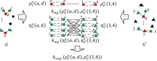
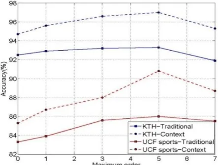
cross-validation. Fig. 1 shows an example of the contexts of primary walk groups, the corresponding kernels, and the context dependent kernel.

Fig. 1. An example of the contexts of primary walk groups and the corresponding kernels: The left and right columns show two graphs G and G, where the green vertices are the contexts of the red ones (The edges are not shown); The middle column shows the kernels on primary walk groups and the kernels on their contexts, both of which are used to define the context-dependent kernel on primary walk groups. A directed dashed curve denotes a random walk.

2.1.3. Context-dependent random walk graph kernel

The nth-order context dependent walk graph kernel is defined as the mean of the sum of the context dependent walk graph kernels with walk length n:







n n n

g n n cwg G G

i j G G

r

k G G k i j r s

N N , (5)

where n G

N is the number of primary walk groups with length n in graph G, and n G

 is the set of all the

walks with length n in graph G. The normalization by n n G G

N N  takes account of the fact that there are different

numbers of local feature vectors in different graphs. We use a positive weight n

to emphasize the importance of the nth-order context dependent random walk graph kernel. Then, the final graph kernel is defined as:

( , ) n n( , )

g g

n

k G G 



Our context-dependent random walk graph kernel is relevant to the traditional random walk graph kernel and the context-dependent kernel for attributed point sets [13]. The description of their relations is included in Appendix A, which is available online.

2.2. Direct product graph-based computation

In practice, a direct product graph [9] is used to efficiently compute the random walk kernel between two graphs. Correspondingly, we propose to utilize direct product graphs to compute context-dependent random walk graph kernels of different orders.

2.2.1. Direct product graph

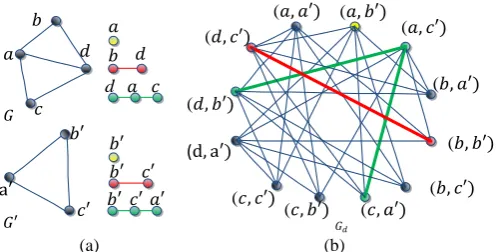
The direct product graph G_d (V E_d, _d) of two graphs G( , )V E and G(V E , ) is a graph whose

vertices are in the set of pairs of the vertices in G and G respectively, as shown in Fig. 2. For a vertex v_i

... a b _c d e f ... 1 4 6

a d 1 4_𝜌

𝐺’ 𝑛 _1,4

b b c c e e f f 2 2 5 5 6 3 3 6

𝜌𝐺𝑛 𝑎, 𝑑

𝜂𝐺𝑛 𝑎, 𝑑 𝜂𝐺’𝑛(1,4)

𝑘𝑤𝑔(𝜌𝐺𝑛 𝑎, 𝑑 , 𝜌𝐺’𝑛(1,4))

𝑘𝑤𝑔(𝜂𝐺𝑛 𝑎, 𝑑 , 𝜂𝐺’𝑛(1,4))

𝑘𝑐𝑤𝑔(𝜌𝐺𝑛 𝑎, 𝑑 , 𝜌𝐺’𝑛(1,4))

𝐺 𝐺′

2

in G and a vertex vr in G, if the vertex kernel k v vv( ,i r) between these two vertices is larger than 0, then

the vertex pair ( ,v vi r) forms a vertex in Gd. For an edge ( ,v vi j) connecting vertices vi and vj in G and

an edge ( ,v v r s) in G, if the edge kernel ke(( ,v vi j), ( ,v vr s)) between these two edges is larger than 0, then

there is an edge connecting vertices ( , )v vi r and ( , )v vj s in Gd. Each vertex ( ,v vi r) in Gd is assigned a

weight w_ir which equals k v vv( ,i r). Each edge (( , ), ( , ))v vi r v vj s in Gd is assigned a weight wir js, which equals k_e(( ,v v_{i j}), ( ,v v_r _s)). For each edge in G_d, there exists a corresponding edge in G and a corresponding edge in G. For each random walk in G_d , there exists a corresponding random walk in G and a corresponding random walk in G, both with the same length.

(a) (b)

Fig. 2. Direct product graph: (a) Two graphs G and G with random walks with different lengths; (b) The corresponding direct product graph and random walks: the yellow, red, and green colors represent, respectively, a 0-order random walk, a 1-order random walk, and a 2-order random walk.

For the direct product graph G_d, we construct a diagonal matrix d d d

V V V





W , in which the ir-th

diagonal element ( , ) d

V

W ir ir is wir, to contain the vertex weights. We construct a matrix

d d d V V E  

W , in

which the element ( , ) d

E

W ir js is wir js, , to contain the edge weights. The nth-order weight matrix

n d W of

d

G is defined as ( )

d d d

n n

d  V E V

W W W W . According to (1),

d d

E V

W W describes the changes in the kernels of

random walks when the walks are extended one edge. Simple derivation yields

( , ) ( ( , ), ( , ))

n n n

d wg G G

W ir js k  i j   r s (For details, see Appendix B, which is available online). Therefore, each

nonzero element in n d

W is the similarity between the corresponding primary walk groups with length n in

graphs G and G, respectively.

2.2.2. Computation of

context-dependent graph kernels of different orders

To represent the context of each vertex in Gd, we define the context matrix

d d

V V d





C whose

elements C ir jsd( , ) are 1 if vj is a context of vi in G and vs is a context of vr in G, otherwise are 0.

Each row in Cd describes the context of one vertex. The nth-order context-dependent weight matrix n cd W of

d

G is computed by n n n ( n T)

cd  d  d d d d

W W W C W C , where is the Hadamard product.

According to (4), each nonzero element in Wcdn corresponds to the context-dependent kernel between

two primary walk groups with length n in graphs G and G respectively, i.e., n( , ) ( n( , ), n( , ))

cd cwg G G

W ir js k  i j   r s ,

where kcwg is defined in (4)(For details, see Appendix B). According to (5), the nth-order context-dependent

𝑎 𝑏 𝑐 𝑑 a′ 𝑏′ 𝑐′

(𝑎, 𝑎′) (𝑎, 𝑏′)

(𝑎, 𝑐′)

(𝑏, 𝑎′)

(𝑏, 𝑏′)

(𝑐, 𝑏′)

(𝑏, 𝑐′)

(𝑐, 𝑎′)

(𝑐, 𝑐′)

(d, a′)

(𝑑, 𝑏′)

(𝑑, 𝑐′)

𝑎

𝑏′

𝑏 𝑑

𝑏′ 𝑐′

𝑎

d 𝑐

𝑎′

𝑏′ 𝑐′

𝐺

walk graph kernel on graphs G and G is rewritten as: , 1 ( , ) ( , )   



g n n cd

ir js G G

k G G W ir js

N N . (7) It is apparent that n n

G G

N N  equals to the number of the nonzero entries in Wcdn. The computational complexity

of the context-dependent walk graph kernel can be found in Appendix C.

2.3. Generalized multiple kernel learning

Substitution of (7) into (6) yields the final graph kernel between two graphs. The weights {n} in (6)

can be estimated using the labeled samples. We apply the generalized multiple kernel learning [19] to this estimation. The multiple kernel learning is an information fusion method. Each type of information corresponds to one kernel. We use the multi-kernel learning to combine the graph kernels of different orders.

In real applications, each sample can be represented by a set of L graphs { }Gl Ll₁ which have the same

vertex set, where different graphs represent different characteristics of these vertices (In our action recognition method, L equals 2, i.e., a concurrent graph and a causal graph are used to represent a sample, as described in Section 4.1). It is apparent that the L graphs share the same 0th order kernel 0

g

k . Let Zl be the maximal order

of the context-dependent walk group kernels on graphs l. The kernel on any two samples S and S is defined as: 0 0 1 1 1 1 ( , ) ( , ) ( , ) l Z L z z

g l g l l

l z

k S S  k G G  k G G

 

   



where the { (z , )}Zl₀

g l l z

k G G _ are computed by (7).

It is assumed that a set of M training samples { }M₁ m m

S _ is available with labels { }M₁ m m

y _ . We define a set

of M×M kernel matrices 0

1 1 { ,{ z} }Zl L

l z l

K K for the training samples, where 0 0

, ,

( , ) ( , )

i j

i j g l S l S

K S S k G G and

, ,

( , ) ( , )

i j

z z

l i j g l S l S

K S S k G G . Corresponding to (8), we define the kernel matrix K for the training samples as

follows: 0 0 1 1 l Z L z z l l l z      



K K K , (9)

where lz0 is the weight for

z l

K . Let Λ be the weight vector whose elements are 0 1,.., 1,...,

{ ,{ z}z Zl}

l l L

  

 . Let Y

be an M×M diagonal matrix with the numbers indicating the sample labels { } 1

M m m

y  on the diagonal. Let 1 be

an M-dimensional vector in which all the entries are 1. The dual problem of generalized multi-kernel learning [19] is represented as minimizing the objective function D( ) which is defined as:





2

1

( ) max

Subject to 0, 0 ,

T T T m D C      

α 1 α α YKYα

1 Yα



(10)

where ( ) 1

M m m

 



α is the Lagrangian multiplier vector, C1 is a constant controlling the importance of the loss,

andthe weights { } are included in K and Λ.

samples. So, we add a sparseness constraint on the weights of those kernels. On the other hand, different graphs preserve different relations between vertices, and contain complementary information. So, we add a smoothness constraint on the weights of the kernels from different graphs (the L graphs for each sample), as well as the weight for the 0-th order context dependent walk graph kernel. Therefore, we propose a l1,2-norm

regularization on the kernel weights Λ. It is defined as:

1

2

0 1 1 1

1 1

1 1 1 12

1

( ) , ( ,..., ) ,.., ( ,..., ) ,..., ( ,..., ) . 2

l L

Z

Z Z

l l L L

rΛ         (11)

We add the l1,2-norm regularization to the generalized multiple kernel learning framework. The objective

function D( )Λ is updated by:





2 2

( ) max T T ( )

D   C r

α

Λ 1 α α YKYα Λ , (12)

where C2 is the constant controlling the regularization on kernel weights.

We utilize the mini-max optimization algorithm [19] to calculate Λ. The details of the algorithm can be found in Appendix D. After the weights in Λ are obtained, the similarities between samples are computed using (8). These similarities are used to train a SVM-based classifier. SVMs are appropriate for graph kernel-based recognition, because SVMs only need to input similarities between samples. The extraction of feature vectors from samples is avoided. Furthermore, SVMs allow for parallel computation of the similarities between samples. Parallel computation is popularly used for action recognition.

3. Tree-Pattern Graph Matching Kernel

Considering that random walks in a graph have simple shapes with chain structures and cannot capture sufficient topological information in a graph, we propose a graph matching kernel based on decomposing graphs into tree patterns which have more complex structure than random walks. The kernel is computed by comparing the incoming and outgoing tree-pattern groups from two graphs. We describe first how to define the tree patterns, then how to recursively measure the kernels for tree-pattern groups, and finally how to construct the tree pattern graph matching kernel.

3.1. Tree patterns

For a directed attributed graph G V E( , ) , each vertex v_iV has a set of incoming neighbors ( )v_i {v_j V| ( , )v v_{j i} E}

 _{  }

and a set of outgoing neighbors ( )v_i {v_jV| ( ,v v_{i j})E}. We define the in-degree of vertex v_i as the number of its in-coming neighbors, and define its out-degree as the number of its out-going neighbors.

A tree is a directed acyclic connected graph. It is denoted as t(U Ft, t) where Ut is its vertex set and

t

F is its edge set. The vertices with in-degree zero are called root vertices. The vertices with out-degree zero are called leaf vertices. Trees are naturally oriented by directed edges from root vertices to leaf vertices. The height ( )h t of a tree t is defined as the maximum number of edges connecting a leaf vertex and a root vertex plus one. The branch ( )b t of a tree is defined as the absolute value of difference between the number of root vertices and the number of leaf vertices. The height and the branch are used to describe the complexity of a tree.

graph is a sub-graph which has a tree structure. In a graph G V E( , ), a tree-pattern which has the same

structure as the tree t(U F_t, _t) is denoted as p_t( ,V E_{t t}) with the vertex set Vt{ ,v vt1 t2,...,vt|Ut|} and the set

t

E of edges linking vertices in V_t, where i

t

v V and |Ut| is the number of vertices in tree t. There is a

one-to-one mapping of vertices and edges between tree pattern p_t and tree t.

Given two tree patterns p_t ( ,V E_{t t}) and p_t( ,V E_t _t) which have the same structure as the tree t, we measure their similarity using the similarities between the vertices and between the edges in the two tree patterns respectively.Let

i

t t

v V and i

t t

vV correspond to the ith vertex of tree t. The tree-pattern kernel

between p_t and p_t is defined as the weighted product of vertex kernels and edge kernels:

| | | |

,

1 1

( , ) _{ }( ) ( , ) ( , )

 

 





t t t v t t e t t

i j

k p p t k v v k e e , (13)

where  1   , ( )

t

h t b

t

 

 _ 

is a weighting function which measures the structure complexity of the tree t. The

complexity of a tree increases when its height h t( ) or its branch b t( ) increases. By adjusting  and γ, the

effect of the complexity of tree patterns on the similarity measurement can be increased or reduced.

(a) Trees (b) Incoming trees (c) Outgoing trees

Fig. 3. Examples of trees with different structures.

We consider incoming trees and outgoing trees. In an incoming tree, the out-degree of all the vertices is one except for the leaf vertex. In an outgoing tree, the in-degree of all the vertices is one except for the root vertex. Fig. 3 shows some examples of incoming and outgoing trees. The tree-patterns extracted from graphs according to incoming trees and outgoing trees are called incoming tree-patterns and outgoing tree-patterns respectively. These two kinds of tree patterns exploit, respectively, the incoming and outgoing neighborhood information on vertices. Let h/ h

in out

T T be the set of incoming/outgoing trees whose heights are less than h. Let

( , )

P t G be the set of tree patterns structured by tree t and extracted from graph G. We define the tree pattern-based h-order graph kernel k G G_gh( , ) between graphs G and G as the summation of the similarities of all the pairs of the incoming and outgoing tree patterns whose heights are less than h:

( , ) ( , )

( , ) ( , )

( , ) ( , ) ( , )

h h

t t

in out

t t

h

g t t t t t t

p P t G p P t G

t T t T

p P t G p P t G

k G G k p p k p p

 

 

   

 

 

 

This new kernel uses incoming and outgoing tree patterns to capture the different local neighborhood relations between vertices. In contrast with random walks, these two types of tree patterns have more complex structures and more effectively describe the local topological structure of graphs for measuring the similarities

h(t)=3, b(t)=0 h(t)=3, b(t)=0 h(t)=2, b(t)=1 h(t)=3, b(t)=2 h(t)=2, b(t)=1 h(t)=3, b(t)=1

between graphs.

3.2. Similarities between tree-pattern groups

By using each vertex as the root of outgoing trees or the leaf of incoming tress, the graph is decomposed into many tree patterns. It is an NP hard problem to extract all the tree patterns from a graph. Instead of extracting all the tree patterns, we recursively compute the similarities between graphs based on tree patterns. This computation depends on the definition of affinal incoming/outgoing tree-pattern groups and incoming/outgoing neighborhood matching sets.

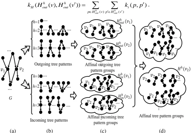
Definition 1: Affinal incoming tree-pattern group: Each vertex v’s h-order affinal incoming tree-pattern group Hinh( )v in a graph G is the set of incoming tree-patterns which have the same leaf vertex v and whose heights are no more than h.

Definition 2: Affinal outgoing tree-pattern group: Each vertex v’s h-order affinal outgoing tree-pattern

group Houth ( )v in a graph G is the set of outgoing tree-patterns which have same root vertex v and whose heights are no more than h.

Fig. 4 shows some examples of affinal incoming/outgoing tree-pattern groups. The similarity between the

affinal incoming tree-pattern groups Hinh( )v for vertex v in graph G and ( )

h in

H v for vertex v in graph G

is defined as the summation of similarities between all the pairs of incoming tree-patterns taken from Hinh( )v and H_inh( )v , respectively. The corresponding kernel is:

( ) ( )

( ( ), ( )) ( , )

h h

in in

h h

H in in t

p H v p H v

k H v H v k p p

 

 

 

 

where k_t() is defined in (13) and the similarity between tree patterns with different tree structures is 0. Similarly, the kernel for affinal outgoing tree-pattern groups is defined as:

( ) ( )

( ( ), ( )) ( , )

h h

out out

h h

H out out t

p H v p H v

k H v H v k p p

 

 

 





(a) (b) (c) (d)

Fig. 4. Examples of affinal tree-patterns: (a) A directed graph G; (b) Incoming tree-patterns and outgoing tree-patterns; (c) Affinal incoming tree-pattern groups and affinal outgoing tree-pattern groups; (d) Affinal tree-pattern groups.

We estimate the h-order affinal tree-pattern group kernel between two vertices using the h-1 order affinal tree-pattern group kernels of the neighbors of the two vertices. We introduce two definitions to exploit the incoming and outgoing neighborhood information in graphs.

𝑣1 𝑣2

... ... ... ... ... ... ... ... ... ... ... ... ... _...

Incoming tree patterns Outgoing tree patterns

𝑣1𝑣1 𝑣1 _...

𝑣2𝑣2 𝑣2 𝑣2 _...

...

Affinal outgoing tree pattern groups

𝑣1

𝑣1

...

𝑣2 𝑣2...

...

𝑣2

𝑣1

Affinal incoming tree pattern groups ... ... h=1 h=2 h=3 h=1 h=2 h=3 G 𝑣1 𝑣2

𝑣1 𝑣1

𝑣1

𝑣1 _𝑣1

𝑣1 𝑣1

...

𝑣1

𝑣1

...

𝑣2 𝑣2 𝑣2 𝑣...2

𝑣2 𝑣2...

𝑣2

𝑣2

...

Affinal tree pattern groups 𝐻𝑜𝑢𝑡ℎ (𝑣1)

𝐻𝑖𝑛ℎ(𝑣1)

𝐻𝑖𝑛ℎ(𝑣2) 𝐻𝑜𝑢𝑡ℎ (𝑣2)

Definition 3: Incoming neighborhood matching set: The incoming neighborhood matching set

( , )

M v v of two vertices v and v in graphs G and G respectively is a set of one-to-one matching pairs of

the incoming neighbors of v and the incoming neighbors of v. An element R of M( , )v v consists of one or

several pair(s) of vertices from incoming neighborhoods ( )v and ( )v of v and v respectively. For pairs (a, b) and (c, d) in R, a is c if and only if b is d, i.e., there is the one-to-one matching between the incoming neighbors of v and v in R. For each vertex pair (a, b) belonging to R, both the vertex kernel on the

pair and the edge kernel on the pair of edges (a,v) and ( , )b v have positive values, i.e., k a bv( , )0 and (( , ),( , )) 0

e

k a v b v  .

Definition 4: Outgoing neighborhood matching set: The outgoing neighborhood matching set

( , )

M v v of two vertices v and v in graphs G and G respectively is defined by replacing the incoming neighborhood in M( , )v v with the outgoing neighborhood, i.e., M( , )v v is a set of one-to-one matching pairs of the outgoing neighbors of v and v.

According to the definition of M( , )v v , by substituting (13) into (15), the affinal incoming tree-pattern group kernel kH(Hinn( ),v Hinn( ))v is rewritten equivalently in a dynamic programming formulation [26] as:













( , ) ( , )

1

( h( ), h( )) , ' 1 ( , ), ( , h ( ), h ( ) ,

H in in v e H in in

u u R R M v v

k H v H v k v v  k u v u v k H u H u

            _     _







where  and  are the two parameters defined in (13) (See [26] for the details of the mathematical

derivation of (17)). Then, the affinal incoming tree-pattern group kernel can be computed recursively. The

initialization for the iteration is 1 1

( ( ), ( )) ( , )

H in in v

k H v H v k v v . Correspondingly, the affinal outgoing tree-pattern group kernel ( n ( ), n ( ))

H out out

k H v H v in (16) is rewritten as:













( , ) ( , )

1

( h ( ), h ( )) , ' 1 ( , ), ( , h ( ), h ( ) ,

H out out v e H out out

u u R R M v v

k H v H v k v v  k v u v u k H u H u

            _     _ 





where 1 1

( ( ), ( )) ( , )

H out out v

k H v H v k v v . In this way, the kernels for affinal tree-pattern groups can be computed efficiently, avoiding the exaction of all the tree patterns in graphs. Verifying whether the tree patterns of two graphs are from the same tree is carried out in the dynamic programming process.

For a vertex v in graph G, the affinal incoming tree-pattern groups Hinh( )v and the affinal outgoing tree-pattern groups h ( )

out

H v are collectively referred to as affinal tree-pattern groups

( ) ( ) ( )

h h h

in out

H v H v H v , as shown in Fig. 4. The kernel ( h( ), h( ))

H

k H v H v between two affinal tree-pattern

groups h( )

H v and h( )

H v is defined as:

( h( ), h( )) ( h( ), h( )) ( h ( ), h ( ))

H H in in H out out

'

( , ) ( ( ), ( ))

h h h

g H

v V v V

k G G k H v H v



 

 

 

This kernel is called the tree-pattern graph kernel. Its computational complexity depends on populating

( , )

M v v and M( , )v v in (17) and (18). Theoretically, its computational complexity is 2 (| || | B) O V V hB , where B is an upper bound on the incoming degree and the outgoing degree. For applications to action recognition, the graphs are very sparse, resulting in a very small value of B. We design the vertex kernel kv() and the edge kernel ke() such that the sizes of the incoming and outgoing neighborhood matching sets are kept small. These designs ensure that the tree-pattern graph kernel is computed efficiently.

The limitation of the tree-pattern graph kernel is that all the similarities between affinal tree-pattern groups are summed up with the same weight. The more discriminative tree patterns are not emphasized.

3.3. Tree-pattern graph matching

To solve the above limitation in the tree pattern graph kernel, we construct a tree-pattern graph matching kernel by finding correctly matched affinal tree-pattern groups using labeled samples.

We assign a weight _{v v,} to each pair of affinal tree-pattern groups Hh( )v and H vh( ) from two

graphs G and G. Then, we define the tree-pattern graph matching kernel h ( , )

mg

k G G for graphs G and G

as follows:

,

( , ) ( h( ), h( ))

mg v v H v V v V

k G G  k H v H v

 

 

 

 

where v v, indicates importance of the matching between ( )

h

H v and H vh( ) .

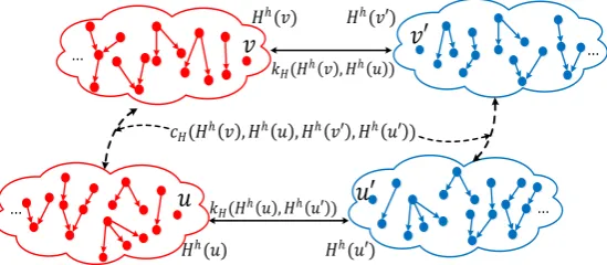
Besides the measurement kH(H v H vh( ), h( )) of the matching quality of a pair of affinal tree-pattern groups Hh( )v and H vh( ) , we define a function cH(H v H u H vh( ), h( ), h( ), H uh( )) to measure the pair-wise agreement between pairs (H v H vh( ), h( )) and (H u H uh( ), h( )) of affinal tree-pattern groups for vertices v and u in G and vertices v and u in G:

( h( ), h( ), h( ), h( )) ( h( ), h( )) ( h( ), h( )) ( , , , ),

H H H

c H v H u H v H u k H v H v k H u H u f v u v u  (22)

where f v u v u( , , , )  measures the geometric relations between pairs of affinal tree-pattern groups and is defined according to applications (see Section 4.2). Fig. 5 shows the relations between pairs of affinal tree-pattern groups.

Fig. 5. The relation between two pairs of affinal tree pattern groups: The quality of a matching pair of affinal tree pattern groups

( )

h

H v and h( )

H v is measured using kH(H v H vh( ), h( )) , and ( ( ), ( ), ( ), ( ))

h h h

H

c H v H u H v H u measures the pairwise

agreement between pairs h( ), h( )

H v H v and h( ), ( )

H u H u .

𝑣

...

𝑢

...

𝑣′

...

𝑢′

... 𝐻ℎ_(𝑣)

𝐻ℎ_(𝑢)

𝐻ℎ_(𝑣′)

𝐻ℎ_(𝑢′) 𝑘𝐻(𝐻ℎ 𝑣 , 𝐻ℎ 𝑢 )

𝑘𝐻(𝐻ℎ 𝑢 , 𝐻ℎ 𝑢′ )

The correctly matched affinal tree-pattern groups have not only high matching degree, but also high pair-wise agreement. The matched affinal tree-pattern groups should be emphasized and the mismatched affinal tree-pattern groups should be suppressed. Given a pair of samples S and S, graph sets

1

{Gl( ,V El l)}lL , and { ( , )} 1

L l l l l

G V E   are extracted respectively. We design a quadratic objective function

for S and S as follows:









, , , ,

{ }

, , , ,

,

max ( ), ( ) ( ), ( ), ( ), ( ) ( )

. . , , 0 1,

h h h h h h

v v H l l v v u u H l l l l v v

l v v l v v u v u v l v v

l l v v

k H v H v c H v H u H v H u C

s t v V v V

    



   

    



    

 

    



 

 

(23)

where C is a constant for the l1,2-norm sparse constraint for selecting matched affinal tree-pattern groups from

the same graphs (the lth graphs) and smoothing the weights of the affinal tree-pattern groups from different graphs (the L graphs for each sample). We determine the weights {_{v v,}} by solving the quadratic objective function in (23) for two samples efficiently using the trust region reflective algorithm [25]. The obtained weights { } are substituted into (21) to compute the tree-pattern graph matching kernel between samples S

and S. The sparse regularization ensures that only the correctly matched affinal tree-pattern groups with high weights are dominant in the kernel construction. This augments the discriminative ability of the tree-pattern graph matching kernel. The kernel similarities between the training samples are used to train a SVM classifier. Given a test sample, we compute its kernels to the support vectors which are a small subset of

the training samples that lie on the maximum margin hyper-planes in the feature space. These kernels are

input to the classifier to determine the label of the test sample. The trust region reflective algorithm requires only a few iterations to obtain an effective local solution and a good classification result, even though the algorithm is halted before convergence.

3.4. Relevance to existing kernels

The proposed tree-pattern graph matching kernel has properties from graph kernels and from graph matching kernels. The corresponding analysis is as follows:

The tree-pattern graph matching kernel extends several previous kernels. When all the weights {v v,} are set to 1, the tree-pattern graph matching kernel reduces to the tree-pattern graph kernel in (20). If we only consider outgoing tree-patterns and set k_v and k_e equal to Dirac kernel functions, then the tree-pattern graph matching kernel reduces to the tree graph kernel in [26]. If parameter  in (13) is very small, then

tree-patterns with a high complexity are penalized, with the result that only tree-patterns consisting of linear chains of vertices have significant weights, i.e., the tree-pattern graph kernel approximates to a traditional random walk graph kernel [20]. If μ in (13) is set to 0, then tree-patterns degenerate into vertices and the tree-pattern graph matching kernel reduces to the summation kernel of vertices [27].

The objective function for determining the weights _{v v,} in (23) is related to the graph matching kernel

in [28, 29, 30, 31]. In both cases, a unary term and a pair-wise term exploit the local compatibilities and pair-wise geometric relations between substructures of graphs. In contrast with traditional graph matching kernels, our tree-pattern group matching kernel has the following properties:

 The tree-pattern graph matching kernel uses affinal incoming and outgoing tree-pattern groups as

 We add a sparse constraint in (23) to keep well matched affinal tree-pattern sets, and remove noisy ones.

3.5. Comparison with context-dependent random walk graph kernel

We summarize the similarities and differences between the context-dependent random walk graph kernel and the tree-pattern graph matching kernel as follows.

1) Similarities: Both these kernels are constructed by decomposing each graph into sub-graphs and then combining the kernels between the sub-graphs. The sub-graphs into which these two kernels decompose a graph are random walks and tree patterns respectively. These two kernels construct the sub-graph kernels in a similar way: The kernels between sub-graphs are products of the kernels for the vertices and the edges included in the sub-graphs and the graph kernels are sum of the kernels of the sub-graphs into which the graphs are decomposed. They both can be reduced to the traditional random walk graph kernel, as stated in Appendix A and Section 3.4.

2) Differences: Random walks in a graph have simple shapes with chain structures. This limits the ability of random walk kernels to capture sufficient topological information in a graph. Tree patterns have more complex structure and obtain more information about the local topologies of graphs than random walks. A primary walk group is a set of random walks starting at a vertex and ending at another vertex. It describes the local structure as a function of depth, as measured by the edges over which the walk passes. The contexts of a primary walk group supplement the normalized local breadth structure information in the random walk graph kernel. An affinal tree-pattern group is a set of tree-patterns that have the same leaf vertex or the same root vertex. It describes the local structure as a function of both the depth and breadth without normalization. Affinal tree-pattern groups consisting of incoming and outgoing tree-pattern groups describe the local structure both along and against the directions of the edges. Therefore, the tree-pattern graph kernel captures more of the local topological properties of the graphs and more accurately measures similarities of graphs than the context-dependent walk graph kernel. As random walks are more regular, the context-dependent random walk graph kernel can be computed directly and conveniently using the direct product graph. The equation for computing the context-dependent random walk kernel is concise. However, tree-pattern graph matching kernel cannot be computed using the direct product graph. It is recursively computed in a dynamic programming formulation. The recursive solution is elegant. But it requires more runtime than the computation of the context-dependent random walk graph kernel. In addition, the context-dependent random walk graph kernel measures the similarity between two graphs by comparing the pairs of sub-graphs of the graphs, while the tree-pattern graph matching kernel keeps well matched sub-graphs.

4. Action Recognition

We follow the traditional action recognition framework based on points of interest. Given a video containing actions, Dollar’s separable linear filters [4] are utilized to detect the spatiotemporal interest points. The 3D SIFT descriptor [17] is used as the local spatiotemporal feature vector to describe each detected interest point. We construct a concurrent graph and a causal graph to model the relations between local feature vectors. Based on the constructed graphs, the similarities between actions are computed for action recognition.

4.1. Graphs for representing actions

frame. Its vertex set Vc consists of the interest points. We employ the ε-graph method to construct the edge

set E_c. A sparse affinity matrix A_c is defined for G_c. Let ( ,x y t_{i i}, )_i be the image and frame coordinates of the ith interest point. For two interest points i and j in the same frame (t_it_j), if point j is up to point i in the image and their image distance is close enough, then the element A i jc( , ) in Ac is 1. In any other case,

( , )

c

A i j is 0. If A i jc( , )1, ( ,v vi j)Ec. As shown in Fig. 6, Gc is a graph directed from bottom upwards

and without loops1. The 3D SIFT descriptor of a vertex is used as its attributed feature vector for capturing local appearance information. Attributes are attached to edges according to the relative spatial positions of vertices. The relative spatial position of v_j with regard to v_i can be represented by r i j( , )(xjx yi, jyi). Then, we describe the attribute associated with an edge ( ,v v_{i j}) using r i j( , ).

Fig. 6. Graphs for representing actions: (a) A video; (b) Local feature vectors; (c) Concurrent graph; (d) Causal graph.

The causal graph G_s ( ,V E_{s s}) is constructed to model the spatial relations of local feature vectors between frames. Its vertices V_s as well as the associated attributed vectors are the same as in the concurrent graph. We define an affinity matrix As for Gs. For two interest points i and j in neighboring frames, if they

are close in the image coordinate space, then element A i js( , ) in As is 1. In any other case, A i js( , ) is 0.

When A i js( , )1, ( ,v vi j)Es. As shown in Fig. 6, Gs is a graph directed from left to right. The attribute

associated with edge e_ij is also described by r i j( , ). While the directed edge e_ij describes a temporal causal relation between v_i and v_j, the assigned edge attribute r i j( , ) describes their relative spatial position.

The concurrent graph and the causal graph describe different relations between local feature vectors. These two graphs are complementary to preserve the spatiotemporal features of actions.

4.2. Action similarity measurement

We apply the proposed context-dependent random walk graph kernel and tree pattern graph matching kernel to measure the similarity between human actions represented by the concurrent graph and the causal graph. This similarity measurement is based on two basic kernels: the vertex kernel and the edge kernel.

In a concurrent graph, let d and d be the 3D SIFT descriptors for vertices v and v, respectively. If the

1

Any one of the following ways can be used to construct a directed concurrent graph: directed from bottom up, directed from top down, directed from left to right, or directed from right to left. If any two of the four ways are combined, then loops may exist in the graph, and loops may produce traceback in random walks.

...

1 t

1 t

2 t

2 t

2 t 1 t

3

t

3

t

3

t 4

t

4

t

4 t

t

t

...

(a)

(b)

(c)

distance between d and d is close in the feature space, then the vertex kernel between them is:

2 2 2

( , ) exp

2

v

d d

k v v



   

 

  

 

 

(24)

where σ is a scale parameter for the Gaussian function. Otherwise, k v v_v( , ) is 0. Given the attributes r i j( , ) of an edge e_ij in a concurrent graph, the edge kernel depends on the spatial distance between vertices v_i and vj and the direction of r i j( , ). The edge kernel k e ee( ,ij oq ) between edge eij in graph G and edge eoq

in graph G is 1, if vectors r i j( , ) and r o q( , ) have similar lengths and directions where the direction similarity is evaluated by the cosine of the angle between r i j( , ) and r o q( , ):

2 2

( , ) ( , ) ( , ) ( , ) r i j r o q r i j r o q



. (25)

Otherwise, k e ee( ,ij oq ) is 0.

The vertex kernel for the causal graph is defined in the same way as in the concurrent graph. The edge kernel k e e_e( ,_{ij oq} ) between edge e_ij in causal graph G and edge e_oq in causal graph G is 1, if vectors

( , )

r i j and r o q( , ) have similar directions, otherwise the edge kernel is 0.

The above definitions of vertex kernels and edge kernels make the two graphs quite sparse. This speeds up the computation process. There are no cycles in either graph. This suppresses the tottering, halting, and backtracking associated with computing the kernels based on random walks or trees.

For the context-dependent random walk graph kernel, based on the defined vertex kernel and edge kernel, the kernels of different orders between the two videos are computed using (7). The l1,2-norm regularized

generalized multiple kernel learning is used to estimate the weights for the kernels of different orders. Then the similarity between the two videos is computed using (8).

For the tree pattern graph matching kernel, we substitute the defined vertex kernel and edge kernel into (17) and (18) to compute the kernels for the affinal incoming and outgoing tree-pattern groups. Subsequently, we define two variables d_{ij oq,} and _{ij oq,} to describe the relative spatial geometric relations between two vertex pairs v vi, jV and v vo , qV:

, 2

,

2 2

( , ) ( , ) ,

( , ) ( , )

arccos .

( , ) ( , )

ij oq ij oq

d r i j r o q

r i j r o q r i j r o q 

  

 _

 _

 

(26)

If v_i and v_j are in the same frame in a video and v_o and v_q are in the same frame in another video, the geometrical coherence function f in (22) is defined as:

2 2

, ,

2 2

( , , , ) exp

2 2

ij oq ij oq i j o q

d

d f v v v v





 

 

   _  _

 , (27)

where _d and _ are scale parameters. Otherwise, f is 0. This definition of f ensures that the affinal tree-pattern group pairs ( h( ), h( ))

i o

H v H v and ( h( ), h( ))

j q

H v H v are used in measuring the pair-wise