1
Variables and their measurement
This book aims to help people analyze quantitative information. Before detailing the ‘hands-on’ analysis we will explore in later chapters, this introductory chapter will discuss some of the background conceptual issues that are precursors to statistical analysis. The chapter begins where most research in fact begins; with research questions.
A research question states the aim of a research project in terms of cases of interest and the
variables upon which these cases are thought to differ. A few examples of research questions are:
‘What is the age distribution of the students in my statistics class?’
‘Is there a relationship between the health status of my statistics students and their sex?’ ‘Is any relationship between the health status and the sex of students in my statistics class affected by the age of the students?’
We begin with very clear, precisely stated research questions such as these that will guide the way we conduct research and ensure that we do not end up with a jumble of information that does not create any real knowledge. We need a clear research question (or questions) in mind before undertaking statistical analysis to avoid the situation where huge amounts of data are gathered unnecessarily, and which do not lead to any meaningful results. I suspect that a great deal of the confusion associated with statistical analysis actually arises from imprecision in the research questions that are meant to guide it. It is very difficult to select the relevant type of analysis to undertake, given the many possible analyses we could employ on a given set of data, if we are uncertain of our objectives. If we don’t know why we are undertaking research in the first place, then it follows we will not know what to do with research data once we have gathered them. Conversely, if we are clear about the research question(s) we are addressing the statistical techniques to apply follow almost as a matter of course.
We can see that each of the research questions above identifies the entities that I wish to investigate. In each question these entities are students in my statistics class, who are thus the
units of analysis – the cases of interest – to my study.
A case is an entity that displays or possesses the traits of a variable.
In this example, as in many others, the cases are individual people. It is important to bear in mind, however, that this is not always so. For example, if I am interested in retention rates for high schools in a particular area, the cases will be high schools. It is individual high schools that are ‘stamped’ with a label indicating their respective retention rate.
In the research questions listed above, all the students in my statistics class constitute my target population (sometimes called a universe).
A population is the set of all possible cases of interest.
In determining our population of interest, we usually specify the point in time that defines the population – am I interested in my currently enrolled statistics students, or those who completed my course last year as well? We also specify, where relevant, the geographic region over which the population spreads.
For reasons we will investigate later, we may not be able to, or not want to, investigate the entire population of interest. Instead we may select only a sub-set of the population, and this sub-set is called a sample.
A sample is a set of cases that does not include every member of the population.
For example, it may be too costly or time consuming to include every student in my study. I may instead choose only those students in my statistics class whose last name begins with ‘A’, and thus be only working with a sample.
Suppose that I do take this sample of students from my statistics class. I will observe that these students differ from each other in many ways: they may differ in terms of sex, height, age, attitude towards statistics, religious affiliation, health status, etc. In fact, there are many ways in which the cases in my study may differ from each other, and each of these possible expressions of difference is a variable.
A variable is a condition or quality that can differ from one case to another.
The opposite notion to a variable is a constant, which is simply a condition or quality that does not vary between cases. The number of cents in a United States dollar is a constant: every dollar note will always exchange for 100 cents. Most research, however, is devoted to understanding variables – whether (and why) a variable takes on certain traits for some cases and different traits for other cases.
The conceptualization and operationalization of variables
Where do variables come from? Why do we choose to study particular variables and not others? The choice of variables to investigate is affected by a number of complex factors, three of which I will emphasize here.
1.Theoretical framework. Theories are ways of interpreting the world and reconciling ourselves to it, and even though we may take for granted that a variable is worthy of research, it is in fact often a highly charged selection process that directs one’s attention to it. We may be working within an established theoretical tradition that considers certain variables to be central to its world-view. For example, Marxists consider ‘economic class’ to be a variable worthy of research, whereas another theoretical perspective might consider this variable to be uninteresting. Analyzing the world in terms of economic class means not analyzing it in other ways, such as social groups. This is neither good nor bad: without a theory to order our perception of the world, research will often become a jumble of observations that do not tie together in a meaningful way. We should, though, acknowledge the theoretical preconceptions upon which our choice of variables is based. 2.Pre-specified research agenda. Sometimes the research question and the variables to be
investigated are not determined by the researchers themselves. For example, a consultant may contract to undertake research that has terms of reference set in advance by the contracting body. In such a situation the person or people actually doing the research might have little scope to choose the variables to be investigated and how they are to be defined, since they are doing work for someone else.
3.Curiosity-driven research. Sometimes we might not have a clearly defined theoretical framework to operate in, nor clear directives from another person or body as to the key concepts to be investigated. Instead we want to investigate a variable purely on the basis of a hunch, a loosely conceived feeling that something useful or important might be revealed if we study a particular variable. This can be as important a reason for undertaking research as theoretical imperatives. Indeed, when moving into a whole new area of research, into which existing theories have not ventured, simple hunches can be fruitful motivations.
These three motivations are obviously not mutually exclusive. For example, even if the research agenda is specified by another person, that person will almost certainly be operating within some theoretical framework. Whatever the motivation, though, social inquiry will initially direct us to particular variables to be investigated. At this initial stage a variable is given a conceptual definition.
The conceptual definition (or nominal definition) of a variable uses literal terms to specify the qualities of a variable.
A conceptual definition is much like a dictionary definition; it provides a working definition of the variable so that we have a general sense of what it ‘means’. For example, I might define ‘health’ conceptually as ‘an individual’s state of well-being’.
It is clear, though, that if I now instruct researchers to go out and measure people’s ‘state of well-being’, they would leave scratching their heads. The conceptual definition of a variable is only the beginning; we also need a set of rules and procedures – operations – that will allow us to actually ‘observe’ a variable for individual cases. What will we look for to identify someone’s health status? How will the researchers record how states of well-being vary from one person to the next? This is the problem of operationalization.
The operational definition of a variable specifies the procedures and criteria for taking a measurement of that variable for individual cases.
A statement such as ‘a student’s health status is measured by how far in meters they can walk without assistance in 15 minutes’ provides one operational definition of health status. With this definition in hand I can start measuring the health status of students in my statistics class by observing distance covered in the set time limit.
The determination of an operational definition for a variable is a major, if not the major, source of disagreement in research. Any variable can usually be operationalized in many different ways, and no one of these definitions may be perfect. For example, operationalizing health status by observing a student’s ability to complete a walking task leaves out an individual’s own subjective perception of how healthy they feel.
What criteria should be used in deciding whether a particular operational definition is adequate? In the technical literature this is known as the problem of construct validity. Ideally, we look for an operationalization that will vary when the underlying variable we think it ‘shadows’ varies. A mercury thermometer is a good instrument for measuring changes in daily temperature because when the underlying variable (temperature) changes the means of measuring it (the height of the bar of mercury) also changes. If the thermometer is instead full of water rather than mercury, variations in daily temperature will not be matched by changes in the thermometer reading. Two days might actually be different in temperature, without this variation being ‘picked up’ by the instrument. Coming back to our example of health status, and relying on an operational definition that just measures walking distance covered in a certain time, we might record two people as being equally healthy, when in fact they differ. Imagine two people who each walk 2200 meters in 15 minutes, but one of these people cannot bend over to tie their shoelace because of a bad back. Clearly there is variation between the two people in terms of their health – their state of well-being. But this variation will not be recorded if we rely solely on a measure of walking ability.
To illustrate further the ‘slippage’ that can occur in moving from a conceptual to an operational definition, consider the following example. A study is interested in people’s ‘criminality’. We may define criminality conceptually as ‘non-sanctioned acts of violence against other members of society or their property’. How can a researcher identify the pattern of variation in this variable? A number of operational definitions could be employed:
• counting a person’s number of criminal arrests from official records; • calculating the amount of time a person has spent in jail;
• asking people whether they have committed crimes; • recording a person’s hair color.
Clearly, it would be very hard to justify the last operationalization as a valid one: it is not possible to say that if someone’s level of criminality changed so too will their hair color! The other operational definitions seem closer to the general concept of criminality, but each has its own problems: asking people if they have committed a crime may not be a perfect measure because people might not be truthful about such a touchy subject. Counting the number of times a person has been arrested is not perfect – two people may actually have the same level of criminality, yet one might have more recorded arrests because they are a member of a minority group that the police target for arrest. This operationalization may thereby actually be measuring a different variable from the one intended: the biases of police rather than ‘criminality’. Using any of these operational definitions to measure a person’s criminality may not perfectly mirror the result we would get if we could ‘know’ their criminality.
A number of factors affect the extent to which we can arrive at an operational definition of a variable that has high construct validity.
1.The complexity of the concept. Some variables are not very complex: a person’s sex, for example, is determined by generally accepted physical attributes. However, most variables are rarely so straightforward. Health status, for example, has a number of dimensions. At a broad level we can differentiate between physical, mental, and emotional health; two people might be physically well, but one is an emotional wreck while the other is happy and contented. If we operationalize health status by looking solely at the physical dimension of its expression, important differences in this variable may not be observed. Indeed each of these broad dimensions of health status – physical, mental, and emotional – are conceptual variables in themselves, and raise problems of operationalization of their own. If we take physical health as our focus, we still need to think about all of its particular forms of expression, such as the ability to walk, carry weight, percentage of body fat, etc.
2.Availability of data. We might have an operationalization that seems to capture perfectly the underlying variable of interest. For example, we might think that number of arrests is a flawless way of ‘observing’ criminality. The researchers, though, may not be allowed, for privacy reasons, to review police records to compile the information. Clearly, a less than perfect operationalization will have to be employed, simply because we cannot get our hands on the ‘ideal’ data.
3.Cost and difficulty of obtaining data.Say we were able to review police records and tally up the number of arrests. The cost in doing so, though, might be prohibitive, in terms of both time and money. Similarly, we might feel that a certain measure of water pollution is ideal for assessing river degradation, but the need to employ an expert with sophisticated measuring equipment might bar this as an option, and instead a subjective judgment of water ‘murkiness’ might be preferred as a quick and easy measure.
4.Ethics. Is it right to go looking at the details of an individual’s arrest record, simply to satisfy one’s own research objectives? The police might permit it, and there might be plenty of time and money available, but does this justify looking at a document that was not intended to be part of a research project? The problem of ethics – knowing right from wrong – is extremely thorny, and I could not even begin to address it seriously here. It is simply raised as an issue affecting the operationalization of variables that regularly occurs in research dealing with the lives of people. (For those wishing to follow up on this important issue, a good starting point is R.S. Broadhead, 1984, Human rights and human subjects: Ethics and strategies in social science research, Sociological Inquiry, 54, pp. 107–23.)
For these (and other) reasons a great deal of debate about the validity of research centers around this problem of operationalization. In fact, many debates surrounding quantitative research are not actually about the methods of analysis or results of the research, but rather whether the variables have been ‘correctly’ defined and measured in the first place. Unless the operational criteria used to measure a variable are sensitive to the way the variable actually changes, they will generate misleading results.
Scales of measurement
We have, in the course of discussing the operationalization of variables, used the word ‘measurement’, since the purpose of deriving an operational definition is to allow us to take measurements of a variable.
Measurement (or observation) is the process of determining and recording which of the possible traits of a variable an individual case exhibits or possesses.
The variable ‘sex’ has two possible traits, female and male, and measurement involves deciding into which of these two categories a given person falls. This set of categories that can possibly be assigned to individual cases makes up a scale of measurement.
A scale of measurement specifies a range of scores (also called points on the scale) that can be assigned to cases during the process of measurement.
When we construct a scale of measurement we need to follow two particular rules. First, the scale must capture sufficient variation to allow us to answer our research question(s). Take the research questions that I posed at the start of this chapter regarding my statistics students. I may use ‘number of whole years elapsed since birth’ as the operational definition for measuring the ages of students in my statistics class. This produces a scale with whole years as the points on the scale, and will yield a variety of scores for age, given the fact that my students were born in different years. Imagine, though, that I was teaching a class of primary school students; measuring age with this scale will be inadequate since most or all of the students will have been born in the same year. Using a measurement scale for age that only registers whole years will not pick up enough variation to help me meet my objectives; every student in the class will appear to be the same age. I might consider, instead, using ‘number of whole months elapsed since birth’ as the scale of measurement. Age in months will capture variation among students in a primary class that age in years will miss.
This example of the age for a group of students highlights an intrinsic problem when we try to set up a scale to measure sufficient variation for a continuous variable that does not arise when we try to measure a discrete variable.
A discrete variable has a finite number of values.
A continuous variable can vary in quantity by infinitesimally small degrees.
For example, the sex of students is a discrete variable with only two possible categories (male or female). Discrete variables often have a unit of measurement that cannot be subdivided, such as the number of children per household. Other examples of discrete variables are the number of prisoners per jail cell, the number of welfare agencies in a district, and the number of industrial accidents in a given year.
The age of students, on the other hand, is a continuous variable. Age can conceivably change in a gradual way from person to person or for the same person over time. Because of this, continuous variables are measured by units that can be infinitely subdivided. Age, for example, does not have a basic unit with which it is measured. We may begin by measuring age in terms of years. But a year can be divided into months, and months into weeks, weeks
into days, and so on. The only limit is exactly how precise we want to be: years capture less variation than months, and months less than weeks. Theoretically, with a continuous variable we can move gradually and smoothly from one value of the variable to the next without having to jump. Practically, though, we will always have to ‘round off’ the measurement and treat a continuous variable as if it is discrete, and this causes the scale of measurement to ‘jump’ from one point on the scale to the next. The scale is by necessity discrete, even though the underlying variable is continuous.
The use of a discrete measurement scale to measure age, whether we do it in years or months, causes us to cluster cases together into groups. The points on the scale act like centers of gravity pulling in all the slight variations around them that we do not want to worry about. We may say that two people are each 18 years old, but they will in fact be different in terms of age, unless they are born precisely at the same moment. But the slight difference that exists between someone whose age is 18 years, 2 months, 5 days, 2 hours, 12 seconds... and someone whose age is 18 years, 3 months, 14 days, 7 hours, 1 second... might be irrelevant for the research problem we are investigating and we treat them the same in terms of the variable, even though they are truly different. No measurement scale can ever hope to capture the full variation expressed by a continuous variable. The practical problem we face is whether the scale captures enough variation to help us answer our research question.
The second rule of measurement is that a scale must allow us to assign each case into one, and only one, of the points on the scale. This statement actually embodies two separate principles of measurement. The first is the principle of exclusiveness, which states that no case should have more than one value for the same variable. For example, someone cannot be both 18 years of age and 64 years of age. Measurement must also follow the principle of exhaustiveness, which states that every case can be classified into a category. A scale for health status that only had ‘healthy’ and ‘very healthy’ as the points on the scale is obviously insufficient; anyone who is less than healthy cannot be measured on this scale.
Levels of measurement
A scale of measurement allows us to collect data that give us information about the variable we are trying to measure.
Data are the measurements taken for a given variable for each case in a study.
Scales of measurement, however, do not provide the same amount of information about the variables they try to measure. In fact, we generally talk about measurement scales having one of four distinct levels of measurement: nominal, ordinal, interval, and ratio.
We speak of levels of measurement because the higher the level of measurement the more information we have about a variable. These levels of measurement are a fundamental distinction in statistics, since they determine much of what we can do with the data we gather. In fact, when considering which of the myriad of statistical techniques we can use to analyze data, usually the first question to ask is the level at which a variable has been measured. As we shall see there are things we can do with data collected at the interval level of measurement that we cannot do with data collected at the nominal level.
Nominal scales
The lowest level of measurement is a nominal scale.
A nominal scale of measurement classifies cases into categories that have no quantitative ordering.
For example, assume I am interested in people’s religion. Operationally I define a person’s religion as the established church to which they belong, providing the following range of categories: Muslim, Hindu, Jewish, Christian, Other.
Notice that to ensure the scale is exhaustive this nominal scale, like most nominal scales, has a catch-all category of ‘Other’. Such a catch-all category, sometimes labelled ‘miscellaneous’ or ‘not elsewhere counted’, at the end of the scale often provides a quick way of identifying a nominal scale of measurement.
Another easy way to detect a nominal scale is to rearrange the order in which the categories are listed and see if the scale still ‘makes sense’. For example, either of the following orders for listing religious denomination is valid:
Christian Muslim Jewish Hindu Other or
Muslim Jewish Hindu Christian Other
Obviously, the order in which the categories appear does not matter, provided the rules of exclusivity and exhaustiveness are followed. This is because there is no sense of rank or order of magnitude: one cannot say that a person in the ‘Christian’ category has more or less religion than someone in the ‘Hindu’ category. In other words, a variable measured at the nominal level varies qualitatively but not quantitatively: someone in the Christian category is qualitatively different to someone in the Hindu category, with respect to the variable ‘Religion’, but they do not have more or less Religion.
It is important to keep this in mind, because for convenience we can assign numbers to each category as a form of shorthand (a process that will be very useful when we later have to enter data into SPSS). Thus I may code – assign numbers to – the categories of religion in the following way:
1 2 3 4 5
Muslim Jewish Hindu Christian Other
These numbers, however, are simply category labels that have no quantitative meaning. The numbers simply identify different categories, but do not express a mathematical relationship between those categories. They are used for convenience to enter and analyze data. I could just as easily have used the following coding scheme to assign numerical values to each category:
1 5 6 8 9
Muslim Jewish Hindu Christian Other
Ordinal scales
An ordinal scale of measurement also categorizes cases. Thus nominal and ordinal scales are sometimes collectively called categorical scales. However, an ordinal scale provides additional information.
An ordinal scale of measurement, in addition to the function of classification, allows cases to be ordered by degree according to measurements of the variable.
Ordinal scales, that is, enable us to rank cases. Ranking involves ordering cases in a quantitative sense, such as from ‘lowest’ to ‘highest’, from ‘less’ to ‘more’, or from ‘weakest’ to ‘strongest’, and are particularly common when measuring attitude or satisfaction in opinion surveys. For example, assume that in trying to measure age I settle on the following scale:
18 years or less 19 to 65 years Over 65 years
This scale clearly does the task of a nominal scale, which is to assign cases into categories. In addition to this it also allows me to say that someone who is in the ‘19 to 65 years’ category is older than someone in the ‘18 years or less’ category. Put another way, the ‘19 to 65
year-old’ is ranked above someone who is ‘18 years or less’. Unlike nominal data, a case in one category is not only different to a case in another, it is ‘higher’, or ‘stronger’, or ‘bigger’, or more ‘intense’: there is directional change.
Unlike nominal scales, we cannot rearrange the categories without the ordinal scale becoming senseless. If I construct the scale in the following way, the orderly increase in age as we move across the page from left to right is lost:
19 to 65 years Over 65 years 18 years or less
As with nominal data, numerical values can be assigned to the points on the scale as a form of shorthand, but with ordinal scales these numbers also need to preserve the sense of ranking. Thus either of the following sets of numbers can be used:
1 =18 years or less 23 =18 years or less
2 =19 to 65 years or 88 =19 to 65 years
3 =Over 65 years 99 =Over 65 years
Either coding system allows the categories to be identified and ordered with respect to each other, but the numbers themselves do not have any quantitative significance beyond this function of ranking.
One common mistake in statistical analysis is to treat scales that allow either a ‘No’ or ‘Yes’ response as only nominal, when they are almost invariably ordinal. Consider a question that asks participants in a study ‘Do you feel healthy?’ We can say that someone who responds ‘Yes’ is not only different in their (perceived) health level, but they also have a higher health level than someone who responds ‘No’. Practically any question that offers a Yes/No response option can be interpreted in this way as being an ordinal scale.
Interval/ratio scales
Ordinal scales permit us to rank cases in terms of a variable; we can, for example, say that one case is ‘better’ or ‘stronger’ than another. But an ordinal scale does not allow us to say by how much a case is better or stronger when compared with another. If I use the above age scale, I cannot say how much older or younger someone in one category is relative to someone in another category. It would be misleading for me to use the second of the coding schemes above and say that someone in the oldest group has 76 more units of age than someone in the youngest group (i.e. 99 – 23 = 76). The distances – intervals – between the categories are unknown.
Consider, however, if we measure age in an alternative way, by asking each person how many whole years have elapsed between birth and their last birthday. Clearly, I can perform the task of assigning people into groups based on the number of years. I can also perform the task of rank ordering cases according to these measurements by indicating who is older or younger. Unlike nominal and ordinal scales, however, I can also measure theamount difference in age between cases. In this measurement scale the numbers we get do really signify a quantitative value: number of years. It is this ability to measure the distances between points on the scale that makes this method of observing age an interval/ratio scale. An interval scale has units measuring intervals of equal distance between values on the scale. A ratio scale has a value of zero indicating cases where no quantity of the variable is present.
In other words, not only can we say that one case has more (or less) of the variable in question than another, but we can also say how much more (or less). Thus someone who is 25 years old has 7 years more age than someone who is 18 years old; we can measure the interval between them. Moreover, the intervals between points on the scale are of equal value over its whole range, so that the difference in age between 18 and 25 years is the same as the difference in age between 65 and 72 years.
Clearly the numbers on an interval scale do have quantitative significance. Hence these numbers are termed the values for the variable. (In the following chapters we will also refer to the numbers used to represent the categories of nominal and ordinal data as ‘values’ or ‘scores’, so that the terms ‘values’, ‘scores’ and ‘categories’ are used interchangeably. For the reasons we have just outlined this is, strictly speaking, incorrect. However, if we take note that for nominal and ordinal data such values are simply category labels without real quantitative significance, such terminology is not too misleading.)
Notice that an observation of 0 years represents a case which possesses no quantity of the variable ‘age’. Such a condition is known as a true zero point and is the defining characteristic of a ratio scale, as opposed to an interval scale. For example, heat measured in degrees Celsius does not have a ‘true’ zero. There is a zero point, but 0°C does not indicate a case where no heat is present – it is cold but not that cold! Instead, 0°C indicates something else: the point at which water freezes. However, this fine distinction between interval and ratio scales of measurement is not important for what is to follow. We can generally perform the same statistical analyses on data collected on an interval scale that we can on data collected on a ratio scale, and thus we speak of one interval/ratio level of measurement.
The importance of the distinction between nominal, ordinal, and interval/ratio scales is the amount of information about a variable that each level provides (Table 1.1).
Table 1.1 Levels of measurement
Level of measurement Examples Measurement procedure Operations permitted Nominal (lowest level) Sex Race Religion Marital status
Classification into categories Counting number of cases in each category; comparing number of cases in each category Ordinal Social class
Attitude and opinion scales
Classification plus ranking of categories with respect to each other
All above plus judgments of ‘greater than’ or ‘less than’ Interval/ratio
(highest level) Age in yearsPulse rate Classification plus ranking plusdescription of distances between scores in terms of equal units
All above plus other mathematical operations such as addition, subtraction, multiplication, etc.
Source:J.F. Healey, 1993, Statistics:A Tool for Social Research, Belmont, CA: Wadsworth, p. 14.
Table 1.1 summarizes the amount of information provided by each level of measurement and the tasks we are thereby allowed to perform with data collected at each level. Nominal data have the least information, ordinal data give more information because we can rank cases, and interval/ratio data capture the most information since they allow us to measure difference.
Before concluding this discussion of levels of measurement there are two important points to bear in mind. The first is that any given variable can be measured at different levels, depending on its operational definition. We have seen, for example, that we can measure age in whole years (interval/ratio), but we can also measure age in broad groupings (ordinal). Conversely, a specific scale can provide different levels of measurement depending on the particular variable we believe it is measuring; it can be, to some degree, a matter of interpretation. For example, we may have a scale of job types broken down into clerical, supervisory, and management. If we interpret this scale as simply signifying different jobs, then it is measuring job classification and is nominal. If we see this scale as measuring job status, however, then we can hierarchically order these categories into an ordinal scale.
Univariate, bivariate, and multivariate analysis
We have just spent some time discussing the notion of levels of measurement, since the nature of the scales we use to measure a variable affects the kinds of statistical analysis we can perform (as we will see in later chapters). The other major factor involved in determining the analysis we perform is the number of variables we want to analyze. Take, for example, the first research question listed at the start of this chapter, which asks ‘What is the age
distribution of the students in my statistics class?’ This questions is only interested in the way that my students may differ in terms of age; age is the only variable of interest to this question. Since it analyzes differences among cases for only one variable, such a question leads to univariate statistical analysis.
The next two questions are more complex; they are not interested in the way in which students vary in terms of age alone. The second links differences in age with health status, and the third throws the sex of students into the mix. A question that addresses the possible relationship between two variables leads to bivariate statistical analysis, while a question looking at the interaction among more than two variables requires multivariate statistical analysis.
This distinction between univariate, bivariate, and multivariate analyses replicates the way in which statistical analysis is often undertaken. In the process of doing research we usually collect data on many variables. We may collect data on people’s weekly income, their age, health levels, how much TV they watch, and a myriad number of other variables that may be of interest. We then analyze each of these variables individually. Once we have described the distribution of each variable, we usually then build up a more complex picture by linking variables together to see if there is a relationship among them. Everyone probably has a common-sense notion of what it means for two variables to be ‘related to’, or ‘dependent on’, each other. We know that as children grow older they also get taller: age and height are related. We also know that as our income increases the amount we spend also increases: income and consumption are related. These examples express a general concept for which we have an intuitive feel: as the value of one variable changes the value of the other variable also changes.
To further illustrate the concept of related variables, assume, for example, that we believe a person’s income is somehow related to where they live. To investigate this we collect data from a sample of people and find that people living in one town tend to have a low income, people in a different town have a higher level of income, and people in a third town tend to have an even higher income. These results suggest that ‘place of residence’ and ‘income level’ are somehow related. If these two variables are indeed related, then when we compare two people and find that they live in different towns, they are also likely to have different income levels. As a result we do not treat income as a wholly distinct variable, but as somehow ‘connected’ to a person’s place of residence. To draw out such a relationship in the data we collect, we use bivariate descriptive statistics that do not just summarize the distribution of each variable separately, but rather describe the way in which changes in the value of one variable are related to changes in the value of the other variable.
If we do believe two variables are related we need to express this relationship in the form of a theoreticalmodel.
A theoretical model is an abstract depiction of the possible relationships among variables.
For example, the second research question with which I began this chapter is interested in the relationship between the sex and health status of my students. Before analyzing any data I may collect for these variables, I need to specify the causal structure – the model – that I believe binds these two variables together. For this example the model is easy to depict: if there is a relationship it is because a student’s sex somehow affects the student’s health level. It is not possible for the relationship to ‘run in the other direction’; a student’s sex will not change as a result of a change in their health level. In this instance we say that sex is the
independent variable and health status is the dependent variable.
The variation of an independent variable affects the variation of the dependent variables
in a study. The factors that affect the distribution of the independent variable lie outside the scope of the study.
Determining the model that characterizes any possible relationship between the variables specified by our research question is not always so easy. Consider again the example of income and place of residence. We can model the possible relationship between these two variables in many different ways. The simplest way in which two variables can be causally related is through a direct relationship, which has three possible forms.
1. One-way direct relationship with income as dependent. This models the relationship as a one-way street running from place of residence to income (Figure 1.1). We may have a theory that argues job and career opportunities vary across towns and this affects the income levels of people living in those towns. In this case we argue that there is a pattern of dependence with income as the dependent variable and place of residence as the independent variable.
Place of residence
independent
dependentIncomeFigure 1.1 One-way direct relationship with income as dependent
2. One-way direct relationship with place of residence as dependent.Another group of social researchers may disagree with the previous model; they come from another theoretical perspective that agrees there is a pattern of dependence between the two variables, but it runs in the other direction. People with high incomes can choose where they live and will move to the town with the most desirable environment. Thus place of residence is the dependent variable and income is the independent variable (Figure 1.2).
Place of residence
dependent
independentIncomeFigure 1.2 One-way direct relationship with place of residence as dependent
3. Two-way direct relationship with place of residence and income mutually dependent. A third group of researchers may agree that the two variables are related, but believe that both types of causality are operating so that the two variables affect each other. In this model, it is not appropriate to characterize one variable as the independent and the other as the dependent. Instead they are mutually dependent (Figure 1.3).
Place of residence
dependent
dependentIncomeFigure 1.3 Two-way direct relationship with place of residence and income mutually dependent
The important point to remember is that we choose a model based on particular theoretical views about the nature of the world and people’s behavior. These models may or may not be correct. Statistical analysis cannot prove any of the types of causality illustrated above. All it can show is some statistical relationship between observed variables based on the data collected. The way we organize data and the interpretation we place on the results are contingent upon these theoretical presuppositions. The same data can tell many different stories depending on the theoretical preconceptions of the story-teller. For instance, we have presented the three simplest models for characterizing a relationship between two variables.
There are more complex models that involve the relationship between three or more variables. To explore more complex relationships would take us into the realm of
multivariate analysis – the investigation of relationships between more than two variables, which we explore in later chapters. However, it is important to keep in mind when interpreting bivariate results the fact that any observed relationship between two variables may be more complicated than the simple cause-and-effect models described above.
Descriptive statistics
We have discussed some conceptual issues that arise when we plan to gather information about variables. The rest of this book, however, is concerned with data analysis; what do we do with measurements of variables once we have taken them? Usually the first task of data analysis is the calculation of descriptive statistics.
Tolstoy’s War and Peace is a very long book. It would not be possible to do such a book justice in any way other than to read it from cover to cover. However, this takes a lot of time and concentration, each of which may not be readily available. If we want simply to get a gist of the story, a shorter summary is adequate. A summary reduces the thousands of words that make up the original book down to a few hundred, while (hopefully) retaining some of the essence of the story. Of course, the summary will leave out a great deal of detail, and the way the book is summarized for one purpose will be different from the way it is summarized for another. Nevertheless, although much is lost, something is also gained when a book so large is summarized effectively.
The same holds true with research. Most research projects will generate a wealth of information. Presenting the results of such research in their complete form may be too overwhelming for the reader so that an ‘abridged version’ is needed; descriptive statistics
provide this abridged version.
Descriptive statistics are the numerical, graphical, and tabular techniques for organizing, analyzing, and presenting data.
The great advantage of descriptive statistics is that they make a mass of research material easier to ‘read’. By reducing a large set of data into a few statistics, or into some picture such as a graph or table, the results of research can be clearly and concisely presented.
Assume we conduct a survey that gathers the data for the age of 20 students in my statistics class, and obtain the following results:
18, 21, 20, 18, 19, 18, 22, 19, 20, 18, 19, 22, 19, 20, 18, 21, 19, 18, 20, 21
This arrangement of the measurements of a variable is called a distribution. I could present this distribution of the raw data as the results of the research, which, strictly speaking, they are. It is not difficult to see, however, that very little information is effectively communicated this way. It is evident that the raw data, when presented in this ‘naked form’, do not allow us to make any meaningful sense of the variable we are investigating. It is not easy to make any sense about the way age is distributed among this group of students.
We can, alternatively, take this set of 20 numbers and put them through a statistical ‘grinder’, which produces fewer numbers – statistics – that capture the relevant information contained in the raw data. Descriptive statistics tease out some important feature of the distribution that is not evident if we just present the raw scores. One such feature we will focus on in later chapters is the notion of average. For example, we might calculate a single figure for the ‘average’ age and present this single number as part of the results of the research. The measure of ‘average’ chosen will certainly not capture all the information contained in the primary data – no description ever does that – but hopefully it will give a general notion of what the 20 cases ‘look like’ and allow some meaningful interpretation.
We have just introduced the notion of ‘average’ as an important feature of a distribution of scores in which we might be interested. In more technical terms this is one of many
numerical techniques for describing data since it involves the use of mathematical formulas for making calculations from the raw data. There are also a variety of graphs and tables in which data can be represented visually to make the information easier to read. The chapters following Chapter 2 will explore these various methods for describing data.
In all of these chapters we will see that regardless of whether we are using graphs, tables, or numerical techniques as the descriptive statistics we are using to summarize our data, the specific choice among these broad classes of statistics is largely determined by the level of measurement for each variable and whether we are undertaking univariate, bivariate, or
multivariate analysis of the variables. This is why we spent some time in the previous sections discussing these concepts. All of these various ways of describing data are summarized in Table 1.2.
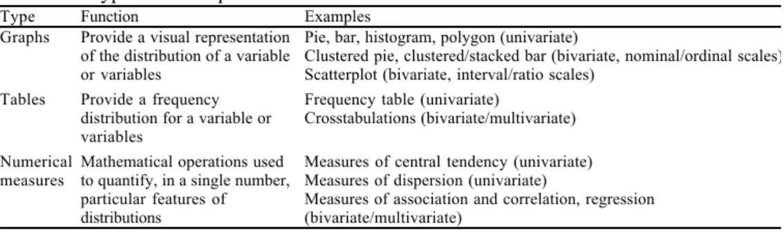
Table 1.2 Types of descriptive statistics
Type Function Examples Graphs Provide a visual representation
of the distribution of a variable or variables
Pie, bar, histogram, polygon (univariate)
Clustered pie, clustered/stacked bar (bivariate, nominal/ordinal scales) Scatterplot (bivariate, interval/ratio scales)
Tables Provide a frequency distribution for a variable or variables
Frequency table (univariate)
Crosstabulations (bivariate/multivariate) Numerical
measures Mathematical operations usedto quantify, in a single number, particular features of distributions
Measures of central tendency (univariate) Measures of dispersion (univariate)
Measures of association and correlation, regression (bivariate/multivariate)
Given the array of descriptive statistics available, how do we decide which to use in a specific research context? The considerations involved in choosing the appropriate descriptive statistics are like those involved in drawing a map. Obviously, a map on the scale of 1 to 1 is of no use (and difficult to fold). A good map will be on a different scale, and identify only those landmarks that the person wanting to cover that piece of terrain needs to know. When driving we do not want a roadmap that describes every pothole and change of grade on the road. We instead desire something that will indicate only the major curves, turn-offs, and distances that will affect our driving. Alternatively a map designed for walkers will concentrate on summarizing different terrain than one designed for automobile drivers, since certain ways of describing information may be ideal for one task but useless for another.
Similarly, the amount of detail to capture through the generation of descriptive statistics cannot be decided independently of the purpose and audience for the research. Descriptive statistics are meant to simplify – to capture the essential features of the terrain – but in so doing they also leave out information contained in the original data. In this respect, descriptive statistics might hide as much as they reveal. Reducing a set of 20 numbers that represent the age for each of 20 students down to one number that reflects the average obviously misrepresents cases that are very different from the average (as we shall see).
In other words, just as a map loses some information when summarizing a piece of geography, some information is lost in describing data using a small set of descriptive statistics: it is a question of whether the information lost would help to address the research problem at hand. In other words, the choice of descriptive statistics used to summarize research data depends on the research question we are investigating.
Exercises
1.1 Consider the following ways of classifying respondents to a questionnaire. (a) Voting eligibility:
• Registered voter
• Unregistered but eligible to vote • Did not vote at the last election (b) Course of enrolment: • Physics • Economics • English • Sociology • Social sciences
(c) Reason for joining the military: • Parental pressure
• Career training • Conscripted
• Seemed like a good idea at the time • No reason given
Do any of these scales violate the principles of measurement? If so, which ones and how?
1.2 What is the level of measurement for each of the following variables? (a) The age in years of the youngest member of each household (b) The color of a person’s hair
(c) The color of a karate belt (d) The price of a suburban bus fare
(e) The years in which national elections were held (f) The postcode of households
(g) People’s attitude to smoking
(h) Academic performance measured by number of marks (i) Academic performance measured as fail or pass (j) Place of birth, listed by country
(k) Infant mortality rate (deaths per thousand)
(l) Political party of the current Member of Parliament or Congress for your area (m)Proximity to the sea (coastal or non-coastal)
(n) Proximity to the sea (kilometers from the nearest coastline) (o) Relative wealth (listed as ‘Poor’ through to ‘Wealthy’) (p) The number on the back of a football player
1.3 Find an article in a journal that involves statistical analysis. What are the conceptual variables used? How are they operationalized? Why are these variables chosen for analysis? Can you come up with alternative operationalizations for these same variables? Justify your alternative.
1.4 For each of the following variables construct a scale of measurement:
(a) Racial prejudice (e) Voting preference
(b) Household size (f) Economic status
(c) Height (g) Aggressiveness
(d) Drug use
For each operationalization state the level of measurement. Suggest alternative operationalizations that involve different levels of measurement.
1.5 Which of the following are discrete variables and which are continuous variables? (a) The numbers on the faces of a die (d) The number of cars in a carpark (b) The weight of a new-born baby (e) Household water use per day (c) The time at sunset (f) Attitude to the use of nuclear power