Qualitative Simulation of Human Resources Subsystem in Software Development Projects

Qualitative Simulation of Human Resources Subsystem in Software

Development Projects

Antonio J. Suarez, Pedro J. Abad

Department of Electronic Engineering, Computer System and Automatic. University of Huelva E-mail: [email protected], [email protected]

Rafael M. Gasca, Juan A. Ortega

Department of Computer Languages and System. University of Sevilla E-mail: [email protected], [email protected]

Abstract

In this paper we presents the inclusion of qualitative arithmetic about planning problem in Software Development projects. Our goal is to simulate subsystem of human resource belonging to the dynamic system of Abdel-Hamid to evaluate its behaviour. We model this subsystem like a CSP(constrains satisfaction problem). Next, we implement this under the constraint programming paradigm as we did in a previous work. This qualitative arithmetic is based on other works [Agell 1998] [Travé-Massuyés 1989] however it is adapted to this particular problem.

All this will serve us to study the possible behaviours of subsystem of human resource along the time, in order to obtain a clear idea of its evolution.

1.- Introduction.

1.1 Qualitative Simulation.

Qualitative simulation is especially useful when we don't have excess or lack of quantitative information in order to simulate a dynamic system.

Qualitative reasoning is considered as one of the discipline of the artificial intelligence. It aims to provide a technique to carry out designs, diagnosis, analysis and simulation where knowledge that we have of the system is little. Qualitative reasoning tries to incorporate the observations coming from the common sense or the intuition. Furthermore, it incorporates the expert’s knowledge, and it gives qualitative explanations of the behaviour of a system based on qualitative descriptions of the possible situations of the real world.

The word dynamic implies that time dependent processes will be the main interesting subjects. Dynamic system

implies that we will study the time behaviour of the system under investigation.

Qualitative simulation predicts the set of possible behaviours of the world. Its value comes from the ability to express natural types of incomplete knowledge of the world, and the ability to derive a probably complete set of possible behaviours in spite of incompleteness of the model.[Kuipers 1994]

Qualitative simulation starts with a qualitative description of real world, and a qualitative description of an initial state. Given a qualitative description of a state, it predicts the qualitative state descriptions that can possibly be next successors of de current state description. Repeating this process produces a graph of qualitative state description, in which the paths starting from the root are the possible qualitative behaviours.[Kuipers 2001]

1.2 Constraint satisfaction problem. (CSP).

Constrains satisfaction problems are those in which you have a set of variables; each of them to be instantiated in an associated domain and a set of Boolean constrains, which limit the set of allowed values for these variables. A constrains satisfaction problem (CSP) is characterized as follow: a set V of n variables {v₁,v₂,....,v_n}, and a domain D_i of possible values associated with each variable v_i, and a set of constraints relations R_i among the variables in the values that these variables can take on. One may be required to find the entire set of solutions or one member of the set or simply to report if the set of solutions has any member. If the set of solutions is empty, the CSP is unsatisfiable. A review about principles of constraint satisfaction can be found in [Miguel & Shen 01]

The use of CSP and qualitative simulation for dynamic systems can be found in [Clancy 98].

1.3 Constraint programming.

Constraint Programming is a problem-solving paradigm that establishes a clear distinction between two pivotal aspects of a problem: a precise definition of the constraints that define the problem to be solved and the algorithms and heuristics enabling the selection of decisions to solve the problem.

A constraint may affect many variables of the system, and these variables may affect another ones. A good form for representing these interactions can be: causal diagrams or Forrester diagrams. ThingLab is an example of such a language where a set of constraints (rules) describes the invariant properties and relationships of all objects in a problem space. The solutions are the set of values that satisfy all the constraints simultaneously.

2. Description of the Problem

For a long time the development software has been an art in hands of the improvisation of the project managers. These projects were carried out taking in account the technical considerations, leaving on a second plane the considerations that had to do with the administration. These administration activities (estimation and planning), were sometimes considered, at the beginning of the project, as a protocol act, with few hopes that they were fulfilled. For project development, the estimation, planning, follow-up and control were carried out without a minimum rigor; most of it was blindly left to the full trust on the intuition and the project manager’s experience. Through the techniques that we expose in the present work, these activities will now have a technological support, since we will apply the above-mentioned techniques.

When the projects were of medium complexity and you could take advantage of the market fever, the enormous deviations in cost and time with regard to initial estimates were considered as something worthless to avoid in a software project.

All software development projects assumed the fact that final cost and timing of delivering the final product were something difficult to compromise.

Projects were more and more complex when the power of the hardware increased and it lowered its cost. This caused that the price of the software began to be important in the total cost for these reasons they need more reliable estimates and planning.

For this reason the project management is one of the focus areas to which process simulation techniques have been applied in the domain of software engineering during the last decade, starting with the pioneering work of Kellner et al. [Kelln 89][Humph 89] and Abdel-Hamid and Madnick [Abdel 91].

Putnam [Putnan 96] defined the estimate of software development like the activity that responds to the questions: how much will it cost? and how long will it be?. Therefore the estimate in software projects consists on predicting the time of the project and the cost that the project will have when it finish.

3. Solution. Appling Constraints

programming to the Dynamic System of

Abdel-Hammid.

3.1 Abdel-Hamid and Manick Dynamic System

The concept of using models to represent engineering systems doesn' t have anything essentially new. In fact, engineering software project managers use mental models in an intuitive way when they make decisions. They select among different alternatives according to the different effect they produce. The relationship that connects the possible actions with its effects, is the system model. On the other hand dynamic systems offer us a way to solve problems where the time is an important factor [Aracil 86]. We will use model of Abdel-Hamid [Abdel 91], which is composed by four subsystems: Software production, Control, Planning and human resources. The relationships among them are shown in the figure 1.

Figure 1: System of Abdel-Hamid and Manick

The software production subsystem takes charge of the basic activities. These activities consist on the assignment of effort, development, quality and tests. On the other hand, the control subsystem takes charge of measuring the progress of the project and making the comparisons with the planning subsystem. The planning subsystem carries out the function of revising and modifying the

initial estimation of the project and this is done according to the information that the system gets from control subsystem. The human resources subsystem, object of our study, is responsible for recruiting, training of selected staff and transfer of human resources among projects.

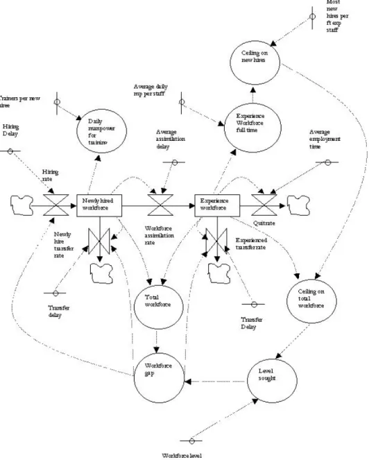
This subsystem is shown in the figure 2. Technicians are divided in two groups: callow technicians and experienced

Figure 2: Subsystem of human resources. .

technicians. This division is necessary for several reasons: Training, productivity, needed effort, rotation.

Training. New members in the project require a period to adapt. Along the period, productivity shows to be low. At the same time, senior staff gives training and company

knowledge to recent comers. This show to be expensive for the company as seniors are not hundred per cent producing

Productivity. Main issue is that the fact mentioned above affects the whole team. The decision to measure the need of effort is taken on an intuitive base.

Necessary effort. To determine the necessary total effort, or what is the same thing, the number of necessary technicians, the project management should consider many factors. Factors to be considered are: effort level needed to complete the project inside the planned limits, remaining tasks and production stability. It is always necessary to keep in mind the phase of the project in which we are. At the end of the project it is more difficult to incorporate personal, although the time and the perceived effort imply this incorporation, this fact would mean longer training time for the organization and the work environment than the project live itself

Rotation. More than a project at a time is normally carried out in software development companies. The rotation of senior from a project to another, plus the need of training for junior by seniors, reduces the ratio of technical full time equivalence senior force.

Remaining time, human resource stability and training requirements will affect the quantity of new human resources that we are looking for.

3.2 Subsystem of Human Resources. Qualitative

Model in Orders of Absolute Magnitude.

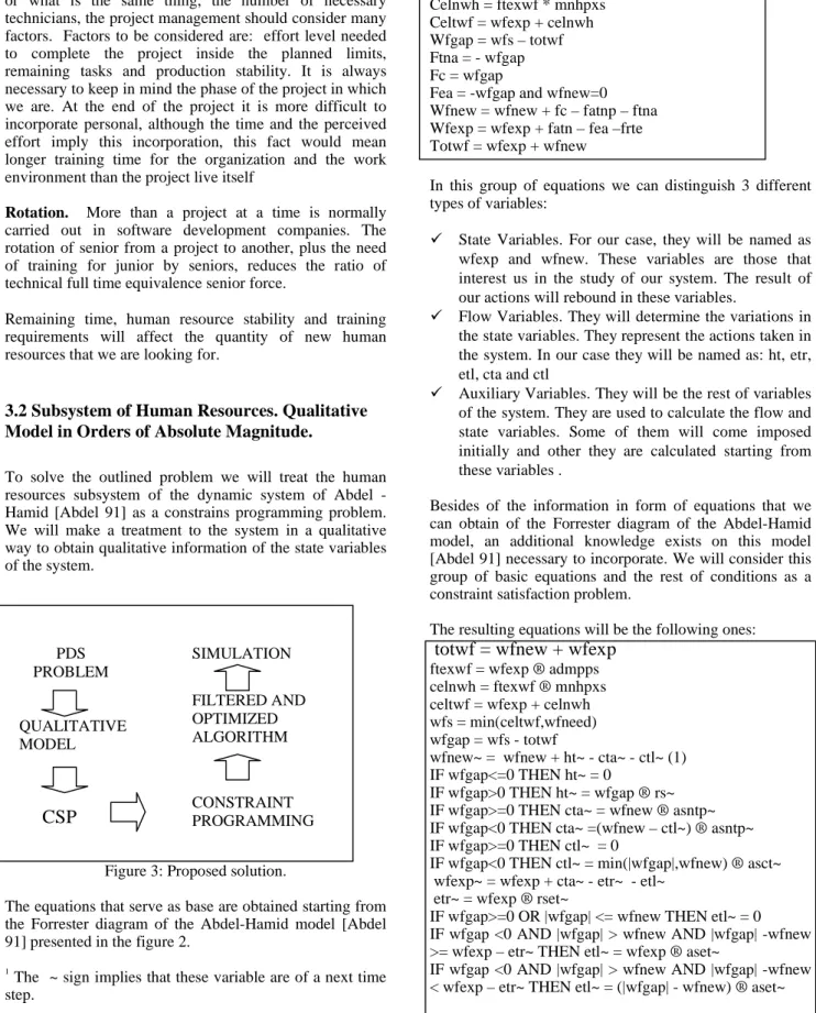
To solve the outlined problem we will treat the human resources subsystem of the dynamic system of Abdel - Hamid [Abdel 91] as a constrains programming problem. We will make a treatment to the system in a qualitative way to obtain qualitative information of the state variables of the system.

Figure 3: Proposed solution.

The equations that serve as base are obtained starting from the Forrester diagram of the Abdel-Hamid model [Abdel 91] presented in the figure 2.

1

The ~ sign implies that these variable are of a next time step.

Celnwh = ftexwf * mnhpxs Celtwf = wfexp + celnwh Wfgap = wfs – totwf Ftna = - wfgap Fc = wfgap

Fea = -wfgap and wfnew=0 Wfnew = wfnew + fc – fatnp – ftna Wfexp = wfexp + fatn – fea –frte Totwf = wfexp + wfnew

In this group of equations we can distinguish 3 different types of variables:

State Variables. For our case, they will be named as wfexp and wfnew. These variables are those that interest us in the study of our system. The result of our actions will rebound in these variables.

Flow Variables. They will determine the variations in the state variables. They represent the actions taken in the system. In our case they will be named as: ht, etr, etl, cta and ctl

Auxiliary Variables. They will be the rest of variables of the system. They are used to calculate the flow and state variables. Some of them will come imposed initially and other they are calculated starting from these variables .

Besides of the information in form of equations that we can obtain of the Forrester diagram of the Abdel-Hamid model, an additional knowledge exists on this model [Abdel 91] necessary to incorporate. We will consider this group of basic equations and the rest of conditions as a constraint satisfaction problem.

The resulting equations will be the following ones:

totwf = wfnew + wfexp

ftexwf = wfexp ® admpps celnwh = ftexwf ® mnhpxs celtwf = wfexp + celnwh wfs = min(celtwf,wfneed) wfgap = wfs - totwf

wfnew~ = wfnew + ht~ - cta~ - ctl~ (1) IF wfgap<=0 THEN ht~ = 0

IF wfgap>0 THEN ht~ = wfgap ® rs~ IF wfgap>=0 THEN cta~ = wfnew ® asntp~ IF wfgap<0 THEN cta~ =(wfnew – ctl~) ® asntp~ IF wfgap>=0 THEN ctl~ = 0

IF wfgap<0 THEN ctl~ = min(|wfgap|,wfnew) ® asct~ wfexp~ = wfexp + cta~ - etr~ - etl~

etr~ = wfexp ® rset~

IF wfgap>=0 OR |wfgap| <= wfnew THEN etl~ = 0 IF wfgap <0 AND |wfgap| > wfnew AND |wfgap| -wfnew >= wfexp – etr~ THEN etl~ = wfexp ® aset~

IF wfgap <0 AND |wfgap| > wfnew AND |wfgap| -wfnew < wfexp – etr~ THEN etl~ = (|wfgap| - wfnew) ® aset~ PDS PROBLEM QUALITATIVE MODEL

CSP

CON

RESTRICCIONE

S

As we can see now, the flow variables, that are those that modify the state variables, don't belong together with the defined ones in the original equations. This has been made this way to be able to introduce the conditions required for the calculation of these variables. The new flow variables will be here named as: ht, cta, ctl, etr and etl. These variables will contain the number of technicians that modify the state variable values wfexp and wfnew.

The flow new variables depend of others that indicate the speed of change of flow variables.

The speed of change indicates the speed with which the technicians are incorporate to the project or they abandon the project. These variables of speed of change will be called here: rset, asntp, rs, asct and aset. When we calculate the flow variables to modify the state variables we will keep in mind that speed.

We have implemented a new operator, here called regulate (represented for ®), with it we can to be able to generate concrete values starting from speed change values. Regulate takes two operands. The first one will be the variable on which it is necessary to act and the second will be the change speed for this variable. This way regulate generates a new flow value for the following time step depending of the change speed of the second operand.

Next we will shortly describe the meaning of each one of the variables of the model.

State Variables

wfexp Experienced WorkForce. It indicates the number of experienced technicians, which there are in the project for each time step. In the initial instant this variable should have a value, because we need to know the number of experienced technicians assigned to the project in a first moment. At the beginning the project we will consider experienced technicians to those that don't need a social training, that is to say, which know the organization

wfnew Newly Hired Workforce. It indicates the number of callow technicians involved in the project. In the initial instant this variable should have a value, because we need to know the number of callow technicians assigned to the project at the beginning. In this instant, since the project is new, we will consider callow technicians those technicians that need a social training and that they do not know the organization.

Flow variables

ht Hired technicians. They will be the number of new technicians that are hired when we need workforce.

etr Experienced technicians that rotate. They are the technicians that are assigned to other projects.

etl Experienced technicians that abandon the project. It will be the number of experienced technicians that should abandon the project. It is not eliminated of the project any experienced technician if there are callow technicians that can be eliminated.

cta Callow technicians those are adapted. They will be the callow technicians that after a time in the project will be considered experienced technicians.

ctl Callow technicians that abandon the project. They will be the number of callow technicians that abandon the project when in the project there are a number of technicians greater than we need.

Auxiliary variables

wfneed Workforce level needed. It comes of another subsystem. It is incorporate to the model in each time step. It provides information of the technicians that we need in that moment for diverse reasons.

mnhpxs Most new hires per full time expert staff. It depends of the number of callow technicians that the experienced technicians can train It will stay stable along of the project lifetime

admpps Average Daily MP per staff. In all organization the norm is that the technicians don't have exclusive dedication to a project. They will have to dedicate part of his time to training, to another projects or to other tasks not related with the project.

rset Rotation Speed of experienced technicians. It indicates the speed to which the experienced technicians change of project.

asntp Adaptation Speed of new technicians to the project. It indicates the speed with which the callow technicians become experienced technicians

rs Recruiting speed. It indicates the velocity with which the technicians are hired. Bureaucratic problems cause that the incorporation of new technicians is never immediate. It will depend on each organization

asct Abandon Speed of the callow technicians. It will indicate the speed with which the callow technicians will abandon the project.

aset Abandon Speed of the experienced technicians. This parameter will indicate us the speed with which the experienced technicians will abandon the project If all the callow technicians have abandoned the project or if none exists is necessary to reduce experienced technicians.

ftexwf Full Time Equivalent Experienced Workforce. Technicians don't usually have total dedication for

different causes. This variable contains the equivalent full time technicians with the current technicians dedication.

celnwh Ceiling on new hires. It will be the maximum number of callow technicians that we can incorporate to the project. It will depend on the maximum limit that the experienced technicians can train.

celtwf Ceiling on Total Workforce. This variable indicates us the maximum number of technicians in the project. It is calculated as the addition of the experienced technicians and the maximum number of technicians to hire.

wfs Workforce level sowght. It is calculated as the minimum of the maximum number of technicians in the project and the number of necessary technicians. Although we need more technicians, we cannot have more technicians than the possible ones.

wfgap Workforce gap. If it is positive we will incorporate technicians to the project, otherwise we should fire to them

totwf Total Workforce. It contains the addition of the state variables wfexp and wfnew

3.3 Qualitative Values Election.

The information that we have of the system is insufficient and quite ambiguous most of the times. In those cases a quantitative treatment of the system is not possible. With the same information, we can achieve a qualitative treatment in most of the cases.

We need a correspondence of integer values with qualitative values to treat the system in a qualitative way. This causes a necessary division of the integer numbers. To carry out this division we won't select a fixed value in the integer numbers. We will simply choose qualitative values and to impose them an order relation. This way any expert will have an idea of what is each one of the qualitative labels for him, without necessity of providing a concrete value for each one of them. A complete study on the treatment in absolute magnitude order can be found in [Agel 98].

It is necessary to assign a correspondence of magnitude among the qualitative labels if we don't want to associate quantitative values to the qualitative labels. The qualitative operators need to know those magnitudes for generating the possible operation results.

Decisions taken when selecting the order and magnitudes of the qualitative labels are the following ones:

As we can see in this situation, we have chosen a symmetrical partition of the integer numbers. Labels PL, PM, NL, NM take values inside the intervals corresponding to the same magnitude. The labels PH and NH take values in open intervals at right and left respectively.

On the other hand, it is necessary to define a correspondence among magnitude and qualitative labels into the interval [0..1].This is caused because in the Abdel-Hammid System there are operations involving integer numbers and numbers into interval [0..1]. This variables are called flow variables.

This treatment is a new approach of the work presented in [Suarez and Abad 2001]

We have resolved correspondence between the qualitative labels and quantitative magnitudes are the following ones:

As we can see in this situation, we have chosen a similar partition of the closed interval [0..1]. Labels FF, FM and FS take values inside the intervals corresponding to the same magnitude.

3.4 Qualitative Operators.

We need to define the operators of the restrictions in a qualitative way because the values of the operands are qualitative also.

The result of the qualitative operations depends of the intervals that we have defined and of the proportions of these intervals in connection with the other ones.

For the qualitative values that have been chosen the definition of qualitative operators will be:

-

∞

-b= -2a -a 0 a b=2a

∞

NH NM NL PL PM PH

FF FM FS

Sum NH NM NL 0 PL PM PH NH NH NH NH NH NM NH - ? NM NH NH NM NH NM NL NM 0 PL NL + NL NH NMN H NLN M NL NL 0 PL PL PM PH PM 0 NH NM NL 0 PL M PH PL NM NH NL NM NL 0 PL PL PL PM PM PH PH PM - NL 0 PL PL PM PM PM PH PH PH PH ? PL PM PH PM PH PH PH PH PH Subtraction NH NM NL 0 PL PM PH NH ? - NM NH NH NH NH NH NM + NL 0 PL NL NM NM NM NH NH NH NL PM PH PL PM NL 0 PL NL NL NM NM NH NH 0 PH PM PL 0 NL NM NH PL PH PM PH PL PM PL NL 0 PL NM NL NM NH PM PH PH PM PH PM PL PM NL 0 PL - PH PH PH PH PH PM PH + ? Regulate 0 PL PM PH 0 0 0 0 0 FS 0 PL PL + FM 0 PL PL,PM + FF 0 PL PL,PM PM,PH

In the operator regulate the columns characterize the variables for regulate and the rows characterize the speed of change of these variables. The result of operation is into interval [0..∞].

4. Model Operating.

We consider a new time step when the values of the state variables change.

For each time step, we need provide the value of the workforce level needed (wfneed) because this variable is generated in another subsystem that is not treat here.

We begin with a series of well-known values of certain variables. We consider these variables as initial parameters of the system. The values of initial parameters will stay constant for all remaining time. Values of the rest of variables, in the initial moment, are calculated for satisfying the defined constraint for that time step.

The values of the variable totwf, for each time step, are the addition of the two state variables values in that time step.

The difference among the variable workforce level sought (wfs) and the variable total workforce (totwf) indicates us the necessity of incorporating technicians or firing technicians for the project. If the variable wfs is greater than the variable totwf we will need to incorporate technicians to the project. If the variable totwf is greater than the variable wfs we will need to fire technicians from the project. Thus, we can know the difference in the number of technicians.

This will cause a modification in the values of the state variables, what takes us to the following time step. For generating the new value of state variables we need to calculate the values of de flow variables previously. The values of the flow variables depends of the numbers of technicians that we need hire or that we need fire and of the value of the speed of change variables for these. Operator regulate returns the values of the flow variables according these two operands. With the new values of the state variables we calculate the values of rest variables. These new variables take the values that complete the imposed restrictions. This way we will have the values of all the variables of the model for that time step. We repeat this process to calculate the following time steps again.

5. Example

To see like the model runs we will give an example.

The initial parameters for the example will be: Variable Value Variable Value

Wfnew PM Wfexp PM

Asntp PH Rset PCERO

mnhpxs PL Wfgap PM

aset PH Asct PH

admpps PH Rs PH

Values of the variable wfneed are in this example:

For time step 0: wfneed = PM For time step 1: wfneed = PL

Predicted behaviour is reduced to around fifty per cent of the possibilities in the worst case and in most cases predicted behaviour is reduced to lest than 33% of the possibilities.

Pos 1 Pos 2 Pos 3 To t1 to t1 to t1 Wfexp PM PM PM PM PM PM Wfnew 0 PL 0 PM 0 PH

6.- Conclusion and Future Works.

We have presented a method for qualitative simulation of subsystem of human resources belonging to system Abdel-Hamid and Madnick system.

We will model this subsystem like a CSP (Constrains satisfaction problem), that is, it will be modelled as a set of restrictions that should be full satisfied. Next, the associated program will be generated under the constraint-programming paradigm.

This simulation of dynamic system provides us all possible behaviours of the subsystem, that is to say, we obtain all valid behaviours but we obtain many non valid behaviours too, this non valid behaviours will be analysed in future works and will try to eliminate them.

In this paper, we have introduced a new operand called regulate. It transforms system variables by using flow variables. Flow variables are into interval [0..1], for this reasons is necessary to define a correspondence among magnitude and qualitative labels into the interval [0..1] and to define the operand regulate.

7. Acknowledgments

This work have been partiality financed by the Comisión Interministerial de Ciencia y Tecnología

(DPI2000-0666-C02-02) y and the Modelización Matemática Redes y Multimedia investigation group of the University of Huelva.

8. References

[Abdel 91] Abdel-Hamid T., Madnick Software Project Dynamics: an integrated approach. 1991, ISBN: 0138220409, Prentice-Hall

[Agel 1998] Agell Jané, N. Estructures matematiques per al model cualitatiu D’ordres de magnitud absoluts. 1998. [Aracil 86] Aracil, J., 1986 Introducción a la Dinámica de Sistemas 1986, ISBN: 84-206-8058-3, Alianza Universidad Textos.

[Clancy 98] Clancy D., Kuipers B. Qualitative simulation as a temporally extended constraint satisfaction problem, In Proc. AAAI 1998

[Humph 89] Humphrey WS, Kellner 1989 MI: Software Process Modeling: Principles of Entity Process Models, Proc.11 th Int’l Conf. Software Engineering (ICSE), IEEE

Computer Soc., pp. 331-342, .

[Kelln 89] Kellner MI, Hansen GA: Software Process Modeling: A Case Study, Proc. 22 nd Annual Hawaii Int’l

[Kuipers 1994]. Benjamin Kuipers. 1989. Qualitative Reasoning . Modeling and Simulation with Incomplete Knowledge. The MIT press.

[Kuippers 2001] Benjamin Kuipers. Qualitative simulation. 2001. Robert A. Meyers, Editor-in-Chief, Encyclopedia of Physical Science and Technology, Third Edition, 2001, NY: Academic Press, pages 287-300..

[Miguel&Shen 01] Miguel, I. and Shen, Q. Solution techniques for constraintsatisfaction problems: Foundations. Artificial Intelligence Review,

15(4):243-267,2001.

[Putnan 96] Putnan L. H., Myers W,; Executive Briefing. Controlling Software Development. IEEE Computer Society Press 1996.

[Suarez&Abad’01] Suárez A., Abad P. Qualitative reasoning for software development project by constraint programming. Third International Conference on Enterprise Information Systems. Setubal 2001.

[Travé-Massuyés 1989] Travé-Massuyés, L. I Piera, N. (1989). The order of Magnitude Models as Qualitative Algebras. A:11th