Open Research Online
The Open University’s repository of research publications
and other research outputs
Contribution of individual variables to the regression
sum of squares
Journal Item
How to cite:
Shabuz, Zillur R. and Garthwaite, Paul H. (2019). Contribution of individual variables to the regression sum of squares. Model Assisted Statistics and Applications, 14(4) pp. 281–296.
For guidance on citations see FAQs.
c
[not recorded]
Version: Accepted Manuscript
Link(s) to article on publisher’s website: http://dx.doi.org/doi:10.3233/mas-190468
Copyright and Moral Rights for the articles on this site are retained by the individual authors and/or other copyright owners. For more information on Open Research Online’s data policy on reuse of materials please consult the policies page.
Contribution of Individual Variables to the Regression Sum
of Squares
Zillur R Shabuza,b and Paul H Garthwaitea∗
a The Open University, Milton Keynes, MK7 6AA,UK b University of Dhaka, Dhaka, Bangladesh
Abstract
In applications of multiple regression, one of the most common goals is to measure the relative importance of each predictor variable. If the predictors are uncorrelated, quantification of relative importance is simple and unique. However, in practice, predictor variables are typically correlated and there is no unique measure of a predictor variable’s relative importance. Using a transformation to orthogonality, new measures are constructed for evaluating the contribution of individual variables to a regression sum of squares. The transformation yields an orthogonal approximation of the columns of the pre-dictor scores matrix and it maximizes the sum of the covariances between the product of individual regressors and the response variable and the cross-product of the transformed orthogonal regressors and the response variable. The new measures are compared with three previously proposed measures through examples and the properties of the measures are examined.
Keywords: Dominance analysis; Orthogonal counterparts; Relative importance; Rel-ative weights; Rotation invariance; Transformation to orthogonality
∗Corresponding author. e-mail: [email protected];
Address: School of Mathematics and Statistics, Open University, Milton Keynes, MK7 6AA,UK Tel: +44 1908 655974
1. Introduction
An important question that statistical consultants and researches commonly face after conducting a multiple regression analysis is which variable contributes most to predict or explain the criterion variable. For example, a chemist may raise the question of the relative importance of temperature and concentration in determining the rate of reaction. The term importance is recognized in the literature as having various possible meanings. A predictor may be considered important if the corre-sponding regression parameter is statistically significant. A second definition judges a predictor as more or less important on the basis of its practical impact on the response. It has been argued that the question of relative importance is even more common than the question of statistical significance (e.g. Healy (1990)).
Numerous methods have been proposed for evaluating the relative importance of regressors. The two most obvious methods are the beta weight method, which simply looks at the beta coefficients of variables that have been standardized to have variances of one, and the zero-order correlation method, which looks at the corre-lation between individual variables and the response. General statistical packages automatically include these statistics in their output from a regression or correlation analysis, making them convenient to use. However, as noted by Lipovetsky and Con-klin (2015), multicollinearity can make these measures practically meaningless since, for example, high collinearity can change signs and inflate the values of regression co-efficients in comparison with pair correlations between the regressors and response. Other evaluation methods include product measures (Pratt, 1987), usefulness (Dar-lington, 1968), structure coefficients (Courville and Thompson, 2001), dominance analysis (Budescu, 1993), orthogonal counterparts (Gibson, 1962; Johnson, 1966), relative weight analysis (Johnson, 2000), Shapley value regression (Lipovetsky and Conklin, 2001) and random forests (Liakhovitski et al., 2010). When predictors are uncorrelated, these measures lead to the same result and have the desirable property that their measures of the individual contributions of the predictor variables sum to R2, the proportion of the variation in the response that the regressors explain.
However, the measures can give quite different results for correlated regressors. Reviews of work on relative importance are given in Johnson and LeBreton (2004), Nathans et al. (2012), Gr¨omping (2007), Lipovetsky and Conklin (2010) and Stadler et al. (2017), and a good older overview is given by Darlington (1968). As
noted by Johnson and LeBreton (2004), there is no unique solution to the problem of evaluating relative importance, so identifying good measures must be based on the logic behind their development, their properties and shortcomings, and the apparent sensibility of the results they yield.
In this paper we develop new measures of relative importance and compare them with well-regarded alternatives. The new measures are based on transformations that yield orthogonal variables that are closely related to the original regressors. In consequence they have much in common with the orthogonal counterparts measure proposed by Gibson (1962) and the relative weights measure of Johnson (2000). The main difference is that the new measures use the values of both the regressors and
the response in determining the transformation, while the measures of Gibson (1962) and Johnson (2000) ignore the response when determining the transformation and use only the values of the regressors. Intuitively, there should be benefits in letting the response influence the transformation, as the purpose of the transformation is to help evaluate the relationship between regressors and the response.
The new measures proposed here are compared with the orthogonal counterparts measure (Gibson, 1962), and the relative weights measure (Johnson, 2000) and also with the dominance analysis measure proposed by Budescu (1993). The relative weights measure and dominance analysis are widely recommended procedures for estimating the relative importance of predictor variables (Tonidandel and LeBre-ton, 2010; Nathans et al., 2012). Comparison is made through examples and by examining theoretical properties.
In Section 2 we describe the measures of Gibson (1962), Johnson (2000) and Budescu (1993) and add insights into these measures. In Section 3 we describe the new measures and in Section 4 they are compared with other measures. Some of the measures have a rotation invariance property, whereby an orthogonal rotation can be applied to some variables without affecting the relative weights assigned to un-rotated variables. The rotation invariance property is described in Appendix A. Concluding comments are given in Section 5.
2. Three Measures of Relative Importance
In this section we describe the orthogonal counterparts measure, the relative weights measure and the dominance analysis measure. The orthogonal counterparts measure
and the relative weights measure each form the basis of new measures that we propose in Section 3.
We assume that the response, Y, and regressors X1, . . . , Xk are related through the regression equation
Y|X =β0+β1X1+. . .+βkXk+ϵ, (1) where X = (X1, . . . , Xk)T and ϵ is random error and has variance σ2. We suppose there are n data, so that the model can be written in matrix form as:
y|X=β01+Xβ+ϵ (2) where1is ann×1 vector of 1’s,y is ann×1 vector of responses,X = (x1, . . . ,xk) is an n×k matrix of known values of X1, . . . , Xk, β is a k×1 vector of regression coefficients (whose values are unknown) and ϵ is an n×1 vector of independent random errors. The coefficient β0 is irrelevant for regressors’ relative importance,
so, to simplify notation, throughout this article we assume that Y and X1, . . . , Xk have been centered to have sample means of 0. Then the least squares estimate of
β is βb = (XTX)−1XTy and var(βb) = σ2(XTX)−1. 2.1 Orthogonal Counterparts (OC) measure
Gibson (1962) and R. M. Johnson (1966) suggested a method for obtaining a set of orthonormal predictors that are closely related on a one-to-one basis with the original set of predictors. The new predictors can be considered as ‘orthogonal counterparts’ to the original regressors. To approximate the relative importance of the original predictors, the response variable is regressed on the new orthonormal variables. The proportion of the predictable variance in the response that is accounted for by each orthogonal counterpart can be taken as the importance measure of the original regressors. Details are as follows.
Suppose a set of orthonormaln×1 vectors z1, . . . ,zk must be chosen to maximise
k
∑
i=1
xTi zi (3)
and let A is the symmetric square-root of XTX. (That is, A is a symmetric matrix whose diagonal elements are positive and AA = XTX.) Then, putting
Z= (z1, . . . ,zk), it can be shown [see, for example, Garthwaite et al. (2012)] that
Z=XA−1. (4)
Each column of Z has a mean of 0 since each column ofX has a mean of 0.
Gibson (1962) and Johnson (1966) assume that the Xi have been standardised to each have the same sample variance, when the maximisation in (3) is equivalent to maximise k ∑ i=1 cor(Xi, Zi), (5) where ‘cor’ denotes sample correlation, and so it is also equivalent to
minimise k ∑ i=1 ˜ ϵTi˜ϵi, (6) where ˜ϵi is the residual when Xi is regressed on a single predictor with sample valueszi. Based on (5), Gibson (1962) describesz1, . . . ,zkas“the set of orthogonal
factors . . . having the highest degree of one-to-one correspondence with the correlated predictors.” Based on (6), z1, . . . ,zk are the best-fitting orthogonal representation of X (Johnson, 2000) and are termed the ‘orthogonal counterparts’ of x1, . . . ,xk. . In the remainder of this paper we will assume that Y and eachX variable have been standardised to have unit length. That is, yTy = xTi xi = 1 for i = 1, . . . , k. LetβbZ = (βbz1, . . . ,βbzk)T denote the vector of regression coefficients from regressing
Y on Z, so βbZ = (ZTZ)−1ZTy = ZTy. Then βbzi is called the beta weight of
Zi (i = 1, . . . , k) and the squared beta weight, βbzi2, is the variation in Y that is explained by Zi. Hence the squared beta weights are a natural measure of the relative importance of theZ variables. EachZ variable is paired with anXvariable, and the Orthogonal Components (OC) measure takes these squared beta weights as a measure of the importance of theX variables, defining the relative importance of Xi as βbzi2. The sum of these importance weights equals the variation in Y that is explained by a multiple linear regression with X1, . . . , Xk as the independent variables (or, equivalently, withZ1, . . . , Zk as the independent variables).
J. W. Johnson (2000) argues that the OC measure can assign relative weights that are inappropriate when the originalXvariables are highly correlated, and gives examples where some variables are assigned weights that seem too low. However, the OC measure appears to give sensible weights to theXvariables when the correlations
between variables are not high. Also, recent work by Garthwaite and Koch (2016) implies that the OC measure has an attractive ‘rotation invariance’ property. When some variables have strong collinearities, they can be transformed into non-collinear variables via orthogonal rotation of coordinate axes. Only axes corresponding to variables involved in the collinearities need to be rotated, and Garthwaite and Koch (2016) show that the rotation has no effect on the Z-variables that correspond to un-rotated axes. The predictable variation inY is also unaffected by the rotation, so the OC measure has the property that the relative importance is unchanged for those X variables associated with un-rotated axes. (Further detail is given in Appendix A.) This has the following implications for the OC measure.
• Sometimes collinear variables can be transformed into meaningful variables that are not collinear through a rotation of the axes associated with them. This can lead to relative weights that are a transparently reasonable representation of the importance of the different variates. Moreover, the relative weights are unchanged for those variables that are not involved in the rotation.
• Since axes could be rotated to remove collinearities without affecting the rela-tive weights of the other variables, multicollinearities do not affect the relative weights that the OC measure gives to variables not involved in the collineari-ties.
Garthwaite et al. (2012) suggest a criterion for choosingz1, . . . ,zkthat is similar, but not identical, to the criterion in (3): Choose ˜z1, . . . ,z˜k to
maximise k
∑
i=1
(xTi z˜i)2 (7)
under the constraint that they are orthonormal vectors and xT
i z˜i > 0 for i = 1, . . . , k. They refer to the transformation fromx1, . . . ,xkto the resulting ˜z1, . . . ,z˜k as the cos-square transformation. It has an attractiveduplicate invariance property.
Suppose the set of vectors {x1, . . . ,xi} is increased by adding the set of vectors {xi+1, . . . ,xk} where each of the vectors xi+1, . . . ,xk is identical to xi. With the cos-square transformation, this duplication of xi has no effect on the transformed values of x1, . . . ,xi−1 (i.e ˜z1, . . . ,z˜i−1 are unchanged.)
Thus, for example, if X1 and X2 are measurements of, say, a patients blood
The duplicate invariance property means that whether one or both blood pressure measurements are included in the regression model has little impact on those Z
variables that are paired with the otherX variables. As the orthogonal Z variables that maximize (3) will generally be very similar to those that maximize (7), we might expect the OC measure to usually be fairly insensitive to variable duplication.
2.2 Relative Weights (RW) measure
The Relative Weights (RW) measure of J. W. Johnson (2000) is based on the same
Z variables that are calculated for the OC measure. That is, z1, . . . ,zk are the orthonormal variables that maximize ∑ki=1xTi zi and, as they are orthogonal, the relative importance of Zi in predicting Y is clearly βbzi2. However, while the OC measure simply takes βbzi2 as the relative importance of Xi, the measure of Johnson (2000) takes into account all the correlations between theX and Z variables. From the criterion that determines the Z variables, the correlation between Xi and Zi should be high, but this correlation could still be well below 1 if the X variables display collinearities or high intercorrelations. Also, Xi might not be the only X variable that has a marked correlation with Zi.
Letλij denote the correlation betweenXi andZj. The transformation fromX to
Z has the unexpected property thatλij =λji for all i, j (see, for example, Johnson (1966)). This leads to the useful consequence that ∑ki=1λ2
ij =
∑k j=1λ
2
ij = 1. The RW measure divides the relative importance ofZjamongst theXvariables according to the square of their correlations with Zj, so the relative importance weight that
Xi derives from Zj is λij2βbzj2 . (This indeed partitions the relative importance of Zj, as ∑ki=1λ2ijβbzj2 = βbzj2.) The full relative importance weight of Xi is obtained by summing the relative importance weights that it derives from all the Z variables. Thus, under the RW measure, the relative importance of Xi is given by
RW of Xi = k ∑ j=1 λ2ijβbzj2 . (8) The λ2
ij in equation (8) may be regarded as the squares of regression coefficients rather than the squares of correlation coefficients, as
1
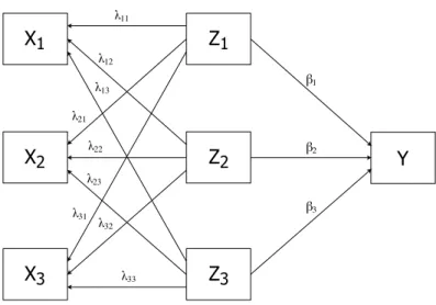
Figure 1 Relationships between theX,Z andY variables for three regressors when
Y is regressed on theZ variables and eachX variable is regressed on theZ variables whenXi is regressed onZ1, . . . , Zk. When Johnson (2000) proposed the RW measure he used the regression model in equation (9) to motivate its construction. However, we prefer to view the λ2
ij as squared correlations because correlation is a symmetric relationship while the regression in equation (9) is a one-directional relationship and shows how the Z variables determine Xi. When viewed as a regression, the rela-tionships between theX, Z and Y variables is illustrated in Figure 1 and shows no direct link between theX andY variables. When the λ2ij are viewed as squared cor-relations, the links between theX and Z variables are two-directional associations, thus giving links from the X variables to Y.
Applications in which the RW measure has been used are reported in Johnson and LeBreton (2004) and Krasikova et al. (2011). Part of the attraction of the RW measure is that it typically gives similar results to the dominance analysis measure of Budescu (1993), even though Budescu’s measure and the RW measure are calculated in very different ways. As Johnson (2000, p.15) suggests, “it is encouraging that two measures that have very different definitions and calculations produce very similar solutions”, and Johnson and LeBreton (2004, p.251) argue that the closeness of results indicates that the two measures are measuring the same construct. We next describe the dominance analysis measure.
2.3 Dominance Analysis (DA) measure
The Dominance Analysis (DA) measure evaluates the importance of a regressor
Xi by considering the increase in R2 that results from adding Xi to regression submodels, whereR2 is the proportion of the variation inY that is explained by the
regression. For correlated regressors, the increase inR2 will generally depend upon
which regressors are in the submodel beforeXi is added. The DA measure considers all the different submodels that could be formed from every possible subset of X
variables that excludes Xi. It defines the weight (relative importance) of Xi as the average increase inR2 from adding Xi to each of these submodels.
The DA measure was proposed by Budescu (1993) and is sometimes referred to as the ‘general dominance measure’. It is equivalent to a measure developed by Lindeman et al. (1980). The measure is well-regarded. For example, Johnson (2000, p.4) writes that “The average increase in R2 associated with the presence of
a variable across all possible models is a meaningful measure that fits the definition of relative weight”. At the same time, it could be argued that the importance of a regressor in a particular regression model should not be determined by its importance in smaller submodels, but by its importance in the full model. As noted earlier, the DA measure and the RW measure are generally very similar in the weights they assign to variables, although an example in Section 4 illustrates that this is not always the case.
The most commonly stated criticism of the DA measure is that it is computa-tionally demanding. This is because there are (2k−1) regression models that should be fitted in order to evaluate the relative importance of each variable. When Linde-man et al. proposed his relative importance measure in 1980, fitting models with all combinations of variables was only practical when the number of variables was fewer than 5 or 6. Since then, advances in computer power has substantially increased that number, so currently it takes only 0.28 seconds to fit all submodels of 12 re-gressors using software developed by Gr¨omping et al. (2006). However, it was not possible to use Gromping’s software with models containing 25 regressors and with 20 regressors the general dominance measure could not be calculated. Moreover, the number of variables that are included in regression models has increased substan-tially, especially with interest in ‘big data’. One possibility is to examine a sample of submodels rather than examining all possible submodels. This approach has proved
effective when using Shapley value regression to measure relative importance (Con-klin et al., 2004), another measure where, in principle, all possible submodels should be examined. Simulations we have conducted suggest that the DA measure can be well-approximated by examining 500 random sequences for entering variables into the regression model.
3 New Measures of Relative Importance
Three new measures are proposed here. All are based on transformations that yield orthogonal variables – the first and third are very similar to the OC measure of Gibson (1962) and R. M. Johnson (1966); the second is very similar to the RW measure of J. W. Johnson (2000). The main difference is that the new measures use transformations that are determined by cross-products of the X and Y variables, rather than ignoringY in choosing the transformation. The third new measure uses weights to alter the balance of the different cross-products when forming orthogonal variables.
The estimated regression coefficientβˆfor regressingY onX = (X1, . . . , Xk)T is
ˆ
β = (XTX)−1XTy (10)
and the regression sum of squares (RegSS) is
yTX(XTX)−1XTy. (11) Let (y1, . . . , yn)T =y and letY be ann×n diagonal matrix with diagonal elements
y1, . . . , yn. The RegSS can also be rewritten as:
1TYXT(XTX)−1XTY1 (12)
where1 is a vector of ones.
Both the OC and RW measures construct orthogonal vectors z1, . . . ,zk that corresponds closely to the original predictorsx1, . . . ,xk on a one-to-one basis. The way the z1, . . . ,zk are chosen ignores the values of Y, even though the reason for constructing z1, . . . ,zk is to partition the RegSS. With our new measures, a set of orthogonal vectors w1, . . . ,wk is chosen so that Ywi is closely related to Yxi. Suppose Y is regressed on w1, . . . ,wk and that wij is the jth component of wi. Then wi’s contribution to the RegSS from the jth sample is (yjwij)2. Our new
measures take (yjwij)2 as a first estimate of the contribution of Xi to the RegSS from thejth sample. (The OC and RW measures equivalently take (yjzij)2 as a first estimate ofXi’s contribution to the RegSS from thejth sample, wherezij is the jth component of zi.) Hence, as yjwij is the jth component of Ywi, it is appropriate to focus on Yw1, . . . ,Ywk in the criterion for choosing w1, . . . ,wk. It is for this reason that we wantYwi and Yxi to be closely related.
We also wantW = (w1, . . . ,wk) to be a linear transformation ofX= (x1, . . . ,xk), so that regression models withw1, . . . ,wkas explanatory variables and withx1, . . . ,xk as explanatory variables give identical predictions, residuals and regression sums of squares. Hence, analogous to equation (3), we chooseWso that∑ki=1(Ywi)T(Yxi) is maximized subject to the constraints that WTW = Ik and W = XC for some
k×k non-singular matrixC. The following result is proved in Appendix B. Theorem 1. Under the constraints that W = XC and WTW = I
k, the value of W= (w1, . . . ,wk) that maximizes ∑k i=1(Ywi) T(Yx i) is W=X(XTX)−1/2G, (13) where G=Ψ(ΨTΨ)−1/2 (14) and Ψ= (XTX)−1/2XTYYX. (15) We should note that theX variables are standardised but||Yxi||typically varies withi. Hence theX variables are given equal importance in maximising ∑ki=1xT
i zi (as with the OC and RW measures) but here, in maximising ∑ki=1(Ywi)T(Yxi),
Xi is given greater importance when ||Yxi|| is large than when it is small. This has the benefit that those X variables that are most highly correlated with Y are given greater weight when choosing thewi. (We could scale theX variables so that ||Yxi|| is the same for each Xi, but that would lose this benefit.)
3.1 First new measure (NM1)
In the same way that the OC measure viewszias the counterpart ofxi(i= 1, . . . , k), our first New Measure (NM1) viewsYwi as the counterpart ofYxi (i = 1, . . . , k). The RegSS when Y is regressed on wi is {1TYwi}2 = (yTwi)2. As {w1, . . . ,wk}
are a set of orthonormal vectors, (yTw
i)2 is the RegSS both when Y is regressed on w1, . . . ,wk and when Y is regressed on x1, . . . ,xk. NM1 defines the relative importance of Xi as
NM1: Relative importance of Xi = (yTwi)2. (16) Like the OC measure, NM1 has a rotation invariance property. Specifically, if an orthogonal rotation is applied to some of theX variables, the relative importance of the other X variables is unchanged if relative importance is measured using NM1. This result is proved in Appendix A, where further detail of rotation invariance is given. As with the OC measure, it means that collinearities do not affect the relative importances that NM1 gives to variables not involved in the collinearities.
3.2 Second new measure (NM2)
While NM1 allocates all the RegSS of Wj to Xj, our second new method, NM2, divides the RegSS of Wj between the X variables according to their association with Wj. As Z =X(XTX)−1/2, from equation (13) we have that W= ZG. (This is an attractive representation ofW because Z is a set of orthonormal vectors and G= (g1, . . . ,gk) is an orthogonal matrix.) Thus,
wj =Zgj, (17) As noted in Section 3, z1, . . . ,zk correspond closely to x1, . . . ,xk on a one-to-one basis, sowj should generally be highly correlated with Xgj. Also, as gi and gj are orthogonal fori̸=j, typicallywj will not be closely associated with Xgi for i̸=j. NM2 divides the RegSS of Wj between X1, . . . Xk to reflect the squares of the sample correlations between Xgi and wj (i = 1, . . . , k). Let rij denote the sample correlation betweenXgi and wj. It is readily shown that
rij = gT i (XTX)1/2gj [gT i XTXgi]1/2 . (18)
The proportion ofWj’s RegSS that NM2 attributes toXi is r2ij/
∑k
ℓ=1rℓj2, so NM2 defines the relative importance ofXi as:
NM2: Relative importance ofXi = k ∑ j=1 r2 ij(yTwj)2 ∑k ℓ=1r2ℓj . (19)
IfXihas low correlations with the otherXvariables, the NM1 and NM2 measures will give similar relative importance to Xi. However the relative importances that they assign to Xi can differ markedly if Xi is highly correlated with some of the X variables. This will be seen in Section 4.
3.3 Third new measure (NM3)
If an X variable has a small regression coefficient in the multiple regression of y
on all the X variables, then dropping that variable from the regression model can be attractive. With the NM1 and NM2 measures (and also the OC and RW mea-sures), the orthogonal counterparts of all variables can change markedly if any X
variables are discarded, which might be undesirable in some situations. Our third new measure, NM3, takes account of the size of regression coefficients when form-ing orthogonal counterparts, so that the inclusion or exclusion of variables with small regression coefficients has little effect on the orthogonal counterparts of other variables.
As in equation (10), let βˆdenote the estimated regression coefficient for regress-ing Y on X = (X1, . . . , Xk)T and put ˆβ = ( ˆβ1, . . . ,βˆk)T. While NM1 and NM2 choose W = (w1, . . . ,wk) to maximize ∑k i=1(Ywi) T(Yx i), with NM3 we choose W# = (w# 1, . . . ,w # k) to maximize ∑k
i=1|βˆi|(Yw#i )T(Yxi). Thus, with NM3, the importance of the correlation between (Yw#i ) and (Yxi) depends upon the size of
ˆ βi. If we letx#i =|βˆi|xi, then ∑k i=1|βˆi|(Yw#i )T(Yxi) = ∑k i=1(Yw # i )T(Yx # i ), and the maximization problem is analogous to the maximisation problem addressed in Theorem 1. PutX# = (x#1, . . . ,xk#). Then replacing Wwith W# and X with X# in equations (13)-(15) yields the value ofW#that maximizes∑k
i=1|βˆi|(Yw#i )T(Yxi). NM3 views (Yw#i ) as the counterpart of (Yx#i ) (i= 1, . . . , k) and evaluates the relative importance ofXi as the value of R2 when Y is regressed on w#i . Thus,
NM3: Relative importance of Xi = (yTw
#
i )
2. (20)
The NM3 and the DA measures are the only measures we examine that explicitly use the multiple regression ofY onX = (X1, . . . , Xk)T. Using this regression model seems sensible, since the purpose of the measures is to evaluate the contribution of each variable to this regression.
4 Examples
In this section we apply the measures of relative importance to several datasets. In Section 4.1 we examine straightforward application of the measures, using three datasets that have clear structures. In Section 4.2 we examine how relative im-portance changes under orthogonal rotation of some variables and under variable selection.
4.1 Fixed models
Each dataset consists of 1000 data drawn from a multivariate normal distribution with a mean vector of zeros and variance-covariance matrix Σ, where Σ varies with the dataset. The first component of a datum is the response, y, and the other components are the explanatory variables, x1, . . . , xk. We first describe each dataset by giving the sample correlation matrix R, the multiple regression modelb that relatesY to the explanatory variables, the value of R2 for that regression, and
the regression coefficients for univariate regressions when Y is regressed separately on one x-variable at a time. We also note salient features of the dataset. After this brief description of the datasets, we tabulate the relative importance that the different measure allocate to each variable. The results are then discussed.
Example 1.
In this first dataset,Y correlates highly withX1 and its correlations withX2 andX3
are much lower. Also, X1 has much the biggest regression coefficient in a multiple
regression of Y onX1,X2. There is marked correlation between the X variables.
The sample correlation matrix is
b R= Y X1 X2 X3 1.000 0.847 0.419 0.382 0.847 1.000 0.701 0.697 0.419 0.701 1.000 0.483 0.382 0.697 0.483 1.000 Y X1 X2 X3
The fitted standardized multiple regression model is: ˆ
and the univariate regression models are ˆ
Y = 0.847X1, Yˆ = 0.419X2, and ˆY = 0.382X3.
Example 2.
There are just two explanatory variables in this dataset. The Y variable is highly correlated with X1 but uncorrelated with Z1. Together, X1 and X2 give a multiple
regression equation that predicts Y perfectly. The sample correlation matrix is
b R= Y X1 X2 1.000 0.893 0.450 0.893 1.000 0.803 0.450 0.803 1.000 Y X1 X2
The fitted standardized multiple regression model is: ˆ
Y = 1.499X1−0.755X2 (R2 = 1.00)
and the univariate regression models are ˆ
Y = 0.893X1, and ˆY = 0.450X2.
Example 3.
In this example, Y is almost a perfect linear function of the last five X variables (X2, . . . , X6) while Y is more highly correlated with X1 than the other X variables.
Also, the largest correlations between theX variables are the correlations involving
X1.
The sample correlation matrix is
b R= Y X1 X2 X3 X4 X5 X6 1.000 0.805 0.681 0.669 0.702 0.702 0.698 0.805 1.000 0.581 0.572 0.601 0.605 0.598 0.681 0.581 1.000 0.352 0.361 0.392 0.386 0.669 0.572 0.352 1.000 0.372 0.384 0.365 0.702 0.601 0.361 0.372 1.000 0.428 0.422 0.702 0.605 0.392 0.384 0.428 1.000 0.400 0.698 0.598 0.386 0.365 0.422 0.400 1.000 Y X1 X2 X3 X4 X5 X6
The fitted standardized multiple regression model is: ˆ
Y = 0.010X1+ 0.277X2+ 0.266X3+ 0.272X4+ 0.261X5+ 0.269X6 (R2 = 0.936)
and the univariate regression models are ˆ
Y = 0.805X1, Yˆ = 0.681X2, Yˆ = 0.669X3
ˆ
Y = 0.702X4, Yˆ = 0.702X5, and ˆY = 0.698X6.
Results from the three examples.
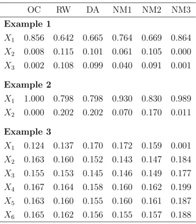
The relative importance given to each variable by the six different measures are given for each example in Table 1. Advocates of the RW measure argue that one of its strengths is that it generally gives similar results to the DA measure. Table 1 shows that this was also the case for our examples, but the table shows that the NM2 measure also gave similar results to DA. Indeed, for Examples 1 and 3 the relative importances assigned by DA are a little closer to those of NM2 than to those of RW. The results of the other measures (OC, NM1 and NM3) are often fairly similar to each other, especially those of OC and NM3, as in Examples 1 and 2. At the same time, NM1 is notably similar to DA in example 3, while NM3 gives radically different results to all other measures in that example.
In each of the examples, at least one variable’s contribution to predictingY was small but it was correlated with variables that were better predictors. Then the variable’s relative importance was generally higher when measured by RW, DA or NM2 than when measured by OC, NM1 or NM3. This can be seen in Example 1, where X2 and X3 are poor predictors, and in Example 2, where X2 is a poor
predictor. The NM1 and NM3 measures, though conceptually quite similar to the OC measure, can give evaluations that are clearly more sensible than those of the OC measure. This is illustrated in Example 2, where the OC measure evaluates the relative importance of X1 as 100% and the relative importance of X2 as 0%. This
is inappropriate, since X1 on its own cannot explain all the variation in Y, while
the combination of X1 and X2 can explain all the variation in Y, clearly showing
that X2 contributes usefully to the multiple regression model. The NM1 and NM3
Table 1: Relative importances given by the orthogonal counterparts (OC), relative weights (RW) and dominance analysis (DA) measures and by three new measures (NM1, NM2 and NM3) in Examples 1–3 OC RW DA NM1 NM2 NM3 Example 1 X1 0.856 0.642 0.665 0.764 0.669 0.864 X2 0.008 0.115 0.101 0.061 0.105 0.000 X3 0.002 0.108 0.099 0.040 0.091 0.001 Example 2 X1 1.000 0.798 0.798 0.930 0.830 0.989 X2 0.000 0.202 0.202 0.070 0.170 0.011 Example 3 X1 0.124 0.137 0.170 0.172 0.159 0.001 X2 0.163 0.160 0.152 0.143 0.147 0.184 X3 0.155 0.153 0.145 0.146 0.149 0.177 X4 0.167 0.164 0.158 0.160 0.162 0.199 X5 0.163 0.160 0.155 0.160 0.161 0.187 X6 0.165 0.162 0.156 0.155 0.157 0.188
given to X2 by the RW, DA and NM2 measures are perhaps a better reflection of
X2’s contribution, since on its own X2 explains 20.3% of the variation in Y.
In Example 3, it is arguable whether X1 is useful for predicting Y. On the
one hand, X1 makes little contribution to the multiple regression model while, on
the other hand, it is the best univariate predictor of Y. NM3 gives X1 a relative
importance that is close to 0, which might be considered appropriate in view of the multiple regression model. Other measures give it a much higher relative importance; indeed, DA and NM1 evaluate it as the most important predictor which, to the writers, seems inappropriate. Example 3 also shows that the RW and DA measures are not always in close agrement: while DA evaluates X1 as the most important
variable in the regression model, RW evaluates it as the least important.
4.2 Orthogonal rotation and variable selection
variables are highly correlated and we consider both the model with the original variables and the model that results from rotating the correlated variables. Measures of relative importance are applied to both models and their differences are examined. In the second example, one variable has a regression coefficient that does not differ significantly from 0 (at the 5% level of significance). We examine how dropping this variable from the model effects the relative importances of the other variables. Example 4. Orthogonal rotation
The Longley dataset (Longley, 1967) is well-used as an example of highly collinear re-gression. The dataset contains annual values of various US macroeconomic variables for the years 1947-1962. Here we use five of its variables: npe (number of thousands of people employed), GN P1 (GNP price deflator), GN P2 (GNP in millions of
dol-lars),npue(number of thousands of unemployed people) andnpa(number of people in the armed forces). We take npe as the response variable and initially take the other four variables as the explanatory variables.
The following is the sample correlation matrix for these variables:
b
R=
npe GN P1 GN P2 npue npa
1.000 0.971 0.984 0.502 0.457 0.971 1.000 0.992 0.621 0.465 0.984 0.992 1.000 0.604 0.446 0.502 0.621 0.604 1.000 −0.177 0.457 0.465 0.446 −0.177 1.000 npe GN P1 GN P2 npue npa
The fitted standardized multiple regression model is:
d
npe= 0.173GN P1+ 0.998GN P2−0.227npue−0.109npa, (21)
for which R2 = 0.986.
The correlation matrix shows that there is a strong collinearity between two of the explanatory variables,GN P1 andGN P2. Collinearity can radically affect the values
of parameter estimates and will inflate their variances. Transforming variables to remove collinearity is consequently attractive and here we replaceGN P1 andGN P2
by the variables X1 = (GN P1+GN P2)/ √ 2 and X1 = (GN P1−GN P2)/ √ 2.
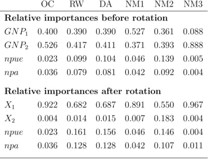
Table 2: Relative importances of variables before and after rotation OC RW DA NM1 NM2 NM3
Relative importances before rotation
GN P1 0.400 0.390 0.390 0.527 0.361 0.088
GN P2 0.526 0.417 0.411 0.371 0.393 0.888
npue 0.023 0.099 0.104 0.046 0.139 0.005
npa 0.036 0.079 0.081 0.042 0.092 0.004 Relative importances after rotation
X1 0.922 0.682 0.687 0.891 0.550 0.967
X2 0.004 0.014 0.015 0.007 0.183 0.004
npue 0.023 0.161 0.156 0.046 0.146 0.004
npa 0.036 0.128 0.128 0.042 0.107 0.011
This is equivalent to multiplying the original variables by the orthogonal rotation matrix, Γ= 1 √ 2 1 √ 2 0 0 1 √ 2 − 1 √ 2 0 0 0 0 1 0 0 0 0 1 .
The new variables X1 and X2 are uncorrelated.
Regressing npe on the transformed set of variables gives the equation
d
npe= 1.681X1−0.054X2−0.227npue−0.109npa. (22)
Theory implies that the regression coefficients of the unrotated components (npue
and npa) should be unchanged – comparison of equations (21) and (22) shows that this is indeed the case. Also, the R2 value is again 0.986. However, with some measures of relative importance, the importances ofnpueandnpain the pre-rotation model (equation (21)) will differ from their importances in the post-rotation model (equation (22)). This can be seen in Table 2, where the relative importances given by our six measures of importance are presented.
In line with theory, the table shows that the relative importances given by the OC and NM1 measures to npue and npa are unchanged by the rotation of GN P1
and GN P2. With the other measures, the relative importances given to npue and
npa do change, though the degree of change varies with the measure. With NM3 the importance values change by a large proportion (e.g. from 0.004 to 0.011), though the changes are small in absolute terms. With the RW and DA measures the changes are quite large - noticeably larger (at least three times larger) than with the NM2 measure. Interestingly, values given by the NM2 measure are straddled by the before/after values given by the RW and DA measures, and are quite close to the averages of the before/after values given by both the RW measure and the DA measure. For example, the RW measure gives before/after values of 0.079 and 0.128 tonpa, and their average is relatively close to the values 0.092 and 0.107 that NM2 gives tonpa.
Example 5. Variable selection
Wood (1973) presents data from a process variable study of a petroleum refinery unit. The dependent variable (Y) is the octane value of the petroleum produced and there are four independent variables: three relate to feed composition (X1, X2, X3)
and the fourth relates to process conditions (X4). Eighty-two observations were
taken, giving the following sample correlation matrix:
b R= Y X1 X2 X3 X4 1.000 −0.870 0.392 −0.638 0.629 −0.870 1.000 −0.589 0.449 −0.337 0.392 −0.589 1.000 −0.298 0.161 −0.638 0.449 −0.298 1.000 −0.722 0.629 −0.337 0.161 −0.722 1.000 Y X1 X2 X3 X4
After centring the variables, regression ofY on the four independent variables gave
b
Y =−0.824X1−0.172X2−0.097X3+ 0.309X4, (R2 = 0.905) (23)
as the regression model. There is clear evidence that X1, X2 and X4 should be
included in the regression model (p < 0.0002 for each of these three variables) but whetherX3 should be included is debatable. The null hypothesis that the regression
coefficient forX3 is zero is rejected only at significance level 0.07. OmittingX3 from
the model gives the regression equation
b
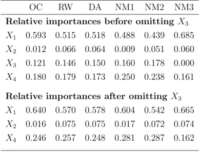
Table 3: Relative importances of variables before and after omittingX3
OC RW DA NM1 NM2 NM3 Relative importances before omitting X3
X1 0.593 0.515 0.518 0.488 0.439 0.685
X2 0.012 0.066 0.064 0.009 0.051 0.060
X3 0.121 0.146 0.150 0.160 0.178 0.000
X4 0.180 0.179 0.173 0.250 0.238 0.161
Relative importances after omitting X3
X1 0.640 0.570 0.578 0.604 0.542 0.665
X2 0.016 0.075 0.075 0.017 0.072 0.074
X4 0.246 0.257 0.248 0.281 0.287 0.162
The top half of Table 3 displays the real importance assigned to the different
X-variables by the different measures when all fourX-variables are included in the regression model. Surprisingly, all but one of the measures givesX3 a higher relative
importance than X2, even though X3 is the variable whose inclusion in the model
is tenuous. The NM3 measure is the exception. It gives X3 a relative importance
of 0.0, which concords fully with the inference that X3 can reasonably be omitted
from the regression model.
The lower half of Table 3 shows the relative importances assigned toX1,X2 and
X4 afterX3 has been omitted from the model. In the whole of the table, the RW and
DA measures are strikingly similar in all their evaluations. It is also the case that all measures evaluateX1 as the most important variable andX2 as the second most
important (both before and after omitting X3). In other respects though, there is
limited agreement across measures. For example, NM1 and NM2 agree quite closely in their evaluations ofX1 andX4, but NM1 is similar to OC in its evaluation ofX2,
while NM2’s evaluations ofX2 are similar to those of RW, DA and NM3.
With most measures, the relative importance ofX3 is far greater than the
differ-ence between the R2 values of the models in equations (23) and (24). Hence, with
those measures the omission of X3 must substantially increase the relative
impor-tance of at least one X-variable. As X3 has higher absolute correlation with X4
relative importance ofX4 more than that of X1 or X2. This is indeed the case for
the OC, RW and DA measures, but not for NM1, NM2 or NM3. It seems then, that the effects on relative importance of omitting a variable are somewhat unpredictable and can vary markedly with the choice of measure.
5 Conclusion
Six measures for evaluating the relative importance of predictor variables in a re-gression have been examined. From the examples presented in Section 4, it is clear that usually there is some consensus between them – variables given a high relative importance by one measure are usually given a high relative importance by other measures, and similarly for low relative importance. At the same time, in each ex-ample there were differences between the measures in their evaluations, and some differences were substantial.
The following correlation matrix combines results from Tables 1–3 to give an overview of the similarity between the different measures. It gives the correlation between each pair of measures for the contributions recorded in Table 1 and the top halves of Tables 2 and 3. (The lower halves of Tables 2 and 3 are ignored to avoid double-counting of data.) OC RW DA N M1 N M2 N M3 OC RW DA N M1 N M2 N M3 1.000 0.981 0.982 0.978 0.981 0.932 0.981 1.000 0.999 0.976 0.988 0.903 0.982 0.999 1.000 0.977 0.990 0.897 0.978 0.976 0.977 1.000 0.984 0.845 0.981 0.988 0.990 0.984 1.000 0.889 0.932 0.903 0.897 0.845 0.889 1.000
The correlations between methods are very high in general, and the correlation between the RW and DA methods is especially high (0.999), showing the high concordance between these two methods that has been found in previous studies (Krasikova et al., 2011; Johnson, 2000). The other striking feature of the corre-lations is the comparatively low correlation between NM3 and each of the other
methods (never exceeding 0.94), indicating that NM3 gives a distinctive perspective on the contributions of variables.
Occasionally, common sense shows that an evaluation is unreasonable. For in-stance, in Example 2 the OC measure evaluated the relative importance of X1 as
100% and that of X2 as 0%. This is clearly inappropriate, as all the variation in Y
could not be explained by X1 on its own, but could be explained by the
combina-tion ofX1 and X2. Often though, the evaluations of the different measures all seem
reasonable and how to choose between them is not clear-cut, because there are no known ‘correct’ evaluations with which to make comparison. As noted by Johnson and LeBreton (2004, page 240), “Because there is no unique mathematical solution to the problem [of evaluating relative importances], these indices [measures] must be evaluated on the basis of the logic behind their development, the apparent sen-sibility of the results they provide, and whatever shortcomings can be identified.” Properties of the different measures and features of the data set should also be taken into account.
The following arguments favour different measures.
1. The DA and RW measures have been the most widely recommended mea-sures in recent years, partly because they typically give similar evaluations, suggesting that there is an underlying construct that they both appraise. The examples presented here support that rationale, as they give further evidence that the two measures generally give similar results – there is only one case (variable X1 in Example 3) where the DA and RW evaluations differ
appre-ciably. The RW measure is simpler and easier to implement than the DA measure.
2. The OC and NM1 measures have the rotation invariance property so, with either measure, multicollinearities have little affect on the relative weights given to variables not involved in the collinearities.
3. In constructing the new measures (NM1–3), the aim was to improve upon the OC and RW measures by letting Y influence the transformation to orthogo-nality, rather than determining the transformation from just the values of the regressors. This was motivated by the observation that the transformation’s purpose is to help evaluate the relationship between Y and the regressors, so
both should be taken into account in forming the transformation. On that basis, NM1 is to be preferred over OC, since in other respects the construction of the two measures are very similar. Similarly for NM2 and RW.
4. In the examples, a feature of NM3 is that it gave low relative importance to variables that might reasonably be omitted from the regression, which could be considered an attractive characteristic. In Example 5, for instance, it gaveX3 a
relative importance of 0.000 while other measures gave it a relative importance of 0.121 or more. Similarly, in Example 3, predictions ofY are not improved by including X1 in the regression model, but only NM3 gaveX1 a low evaluation.
Taking account of the above points, the NM3 measure is recommended when there are some independent variables whose inclusion or exclusion from the regres-sion model is debateable. When it is clear which independent variables should feature in the regression, but there is high multicollinearity among a subset of them, then the NM1 measure is recommended because it has the rotation invariance prop-erty, though its choice in preference to the OC measure (which also has the rotation invariance property) is close. In other circumstances, one of the RW, DA and NM2 measures should be used and we recommend the RW measure – the three measures are likely to give very similar evaluations of relative importance and the RW measure is widely recommended for its simplicity and ease of use (Tonidandel and LeBreton, 2010).
The new measures presented here and ideas behind them could be adapted to give other measures of potential value. In particular, any of the OC, RW and NM2 measures could be modified to use regression coefficients as weights when forming orthogonal counterparts, in the same way that NM3 is derived from NM1. The weighting scheme could also be generalised to use the (|βˆi|)α as weights (where the
βi are the multiple regression coefficients). Setting α equal to 0 would correspond to ‘no weighting’, and increasingα would increase the importance of the weighting. Acknowledgments
We are grateful to a referee whose constructive comments led to clear improvements in the paper.
X1 X1∗ X2
X2∗
Figure 2(a) Points before rotation with
X1,X2 as axes.
X1∗ X2∗
Figure 2(b) Points after rotation with
X1∗,X2∗ as axes.
Appendix A: Rotation invariance property
An orthogonal rotation of axesX1,X2 to axesX1∗, X2∗ is illustrated in Figures 2(a)
and 2(b). In Figure 2(a), the positions of 10 points (x1, x2) are plotted and new
axes X1∗ and X2∗ are shown. The new axes are obtained by rotating the original axes X1 and X2 (by 45o in this case). Figure 2(b) shows the same 10 points, but
drawn with X1∗ and X2∗ as the horizontal and vertical axes. It can be seen that rotation of axes changes the correlation between variables: Figure 2(a) shows that the points are highly correlated when expressed in terms ofX1 andX2, while Figure
2(b) shows that the correlation is low when the points are expressed in terms of
X1∗ and X2∗. Consequently, orthogonal rotation can be used to remove or reduce collinearity between variables.
We only need to rotate those variables that are involved in collinearities. For example, suppose there is just one collinearity and it involves only the first dof the
k explanatory variables. Then axes are rotated using a rotation matrix, Γ say, that has the following block-diagonal form:
Γ= Γd 0 0 Ik−d , (25)
where Γd is an orthogonal matrix of order d and Ik−d is a (k −d) order identity matrix.
predictors. The rotation matrix should be chosen in such a way that the variables that are created have meaningful interpretation. For example, if only the first two predictors X1 and X2 are responsible for one collinearity thenΓd can be set as:
Γd = √12 1 √ 2 −√1 2 1 √ 2 (26)
This rotation creates two meaningful variables, the first one is proportional toX1+
X2 and the second one is proportional to X2−X1.
In terms of the original variables, X1 and X2, the ten points in Figure 2 form
the data matrix:
−0.48 −0.42 −0.24 −0.18 −0.12 0.18 0.18 0.24 0.36 0.48
−0.48 −0.41 −0.41 −0.07 0.07 0.14 0.21 0.14 0.41 0.41
. (27) Post-multiplying this data matrix by Γd in equation (26) gives the points in terms of the new variables X1∗ and X2∗:
−0.68 −0.59 −0.46 −0.18 −0.04 0.22 0.27 0.27 0.55 0.63
0.00 0.01 −0.12 0.08 0.13 −0.03 0.02 −0.07 0.04 −0.05
.
The sample correlation between X1 and X2 is 0.951, while the sample correlation
between X1∗ and X2∗ is 0. (The correlation between the sum and difference of two variables that have been standardised to have equal variances is always 0.)
With the majority of measures of importance, rotating some explanatory vari-ables will change the relative importance of every variable. However, results in Garthwaite and Koch (2016) show that with the OC measure only the relative im-portances of variables involved in the rotation are changed – the relative imim-portances are unchanged for those variables that are not involved in the rotation. Theorem 2 (below) shows that NM1 also has this rotation invariance property.
Lemma 1. If His a positive-definite matrix and Γ is an orthogonal matrix of the same dimension as H, then (ΓTHΓ)−1/2 =ΓTH−1/2Γ.
Proof. (ΓTH1/2Γ).(ΓTH1/2Γ) = ΓTH1/2(ΓΓT)H1/2Γ = ΓTHΓ, so (ΓTHΓ)1/2 = ΓTH1/2Γ. Hence, (ΓTHΓ)−1/2 = (ΓTH1/2Γ)−1 =Γ−1H−1/2(ΓT)−1 =ΓTH−1/2Γ.
Lemma 2. Suppose X∗ = XΓ. Under the constraints that W∗ is a linear trans-formation of X∗ and that (W∗)TW∗ = Ik, the value of W∗ = (w∗1, . . . ,w∗k) that
maximises ∑ki=1(Yw∗i)T(Yx∗ i) is
W∗ =WΓ, (28)
where W is defined by equations (13), (14) and (15).
Proof. Let Ψ∗ = [(X∗)TX∗]−1/2(X∗)TYYX∗ and put G∗ = Ψ∗[(Ψ∗)TΨ∗]−1/2. Now, [(X∗)TX∗]−1/2(X∗)T = [ΓTXTXΓ]−1/2ΓTXT =ΓT[XTX]−1/2ΓΓTXT (from Lemma 1), so
[(X∗)TX∗]−1/2(X∗)T =ΓT[XTX]−1/2XT. (29) Hence, Ψ∗ = ΓT[XTX]−1/2XTYYXΓ = ΓTΨΓ, where Ψ is defined in equa-tion (15). Thus G∗ = ΓTΨΓ[(ΓTΨΓ)(ΓTΨΓ)]−1/2 = ΓTΨΓΓT[ΨΓΓTΨ]−1/2Γ (from Lemma 1), so G∗ =ΓTΨ[ΨΨ]−1/2Γ= ΓT
GΓ, where G is defined by equa-tion (15). Now the proof of Theorem 1 does not require the fact that the X vari-ables have been standardised to have unit variance. Hence the result of the the-orem also applies to W∗ and X∗. It follows that W∗ = (X∗)T[(X∗)TX∗]−1/2G∗ so, from equation (29), W∗ = X[XTX]−1/2ΓG∗. As G∗ = ΓTGΓ, this gives W∗ =X[XTX]−1/2ΓΓTGΓ, so W∗ = WΓ, where W is defined by equation (13).
2
If say, just the first d of k explanatory variables are rotated, then the rotation matrix Γ has the block-diagonal structure in equation (25). Then, from Lemma 2, (w∗d+1, . . . ,w∗k) = (wd+1, . . . ,wk). When Y is regressed on (w∗1, . . . ,w∗k), the con-tribution ofw∗i to the RegSS is the same as the RegSS from a univariate regression ofY on w∗i, because w∗1, . . . ,w∗k are an orthogonal set of vectors. Under NM1, this RegSS is taken as the relative importance ofXi∗ in a regression ofY on (X1∗, . . . , Xk∗). Similarly, when Y is regressed on (X1, . . . , Xk), NM1 evaluates the relative impor-tance of Xi as the RSS from a univariate regression of Y on wi. As w∗i = wi for
i = d+ 1, . . . , k, NM1 has the rotation invariance property given in the following theorem.
Theorem 2. If an orthogonal rotation is applied to some of the X variables, the relative importance of the other X variables is unchanged if relative importance is measured using NM1.
Appendix B: Proof of Theorem 1 Preliminary lemma:
Lemma 3. If W =XC and WTW=Ik, then W=X(XTX)−1/2G where G is a
k×k orthogonal matrix. The converse also holds: if W =X(XTX)−1/2G and G
is an orthogonal matrix, then WTW=I k.
Proof of Lemma 3. For the first part of the lemma, letG= (XTX)1/2C. ThenC= (XTX)−1/2GandW=X(XTX)−1/2G. AlsoI
k=WTW=GT(XTX)−1/2XTX(XTX)−1/2G= GTG. This implies that G is orthogonal, as required. The converse is
imme-diate: if W = X(XTX)−1/2G and G is an orthogonal matrix, then WTW = GT(XTX)−1/2XTX(XTX)−1/2G=GTG=I
k. 2
Proof of Theorem 1. From Lemma 3, W = X(XTX)−1/2G where G is an or-thogonal matrix. Put G = (g1, . . . ,gk), so wi = X(XTX)−1/2gi. Also, de-fine ψi = (XTX)−1/2XTYYx i for i = 1, . . . , k. Then ∑k i=1(Ywi)T(Yxi) = ∑k i=1(g T i (XTX)−1/2XTYT)(Yxi) = ∑k i=1 g T i ψi. As G is an orthogonal matrix, it is immediate from Theorem 1 in Garthwaite et al. (2012) that∑ki=1 gTi ψi is max-imised when G = Ψ(ΨTΨ)−1/2, where Ψ = (ψ
1, . . . ,ψk). Thus equation (15)
definesΨ. 2
References
Budescu, D. V. (1993). Dominance analysis: A new aproach to the problem of relative importance of predictors in multiple regression. Psychological Bulletin, 114:542–551.
Conklin, M., Powaga, K., and Lipovetsky, S. (2004). Customer satisfaction analysis: Identification of key drivers. European Journal of Operational Research, 154:819– 827.
Courville, T. and Thompson, B. (2001). Use of structure coefficients in published multiple regression articles: β is not enough. Educational and Psychological Mea-surement, 61:229–248.