8-19-2014 12:00 AM A Phase-Angle Tracking Method for Synchronization of Single- and Three-Phase Grid-Connected Converters

(1)

Western University Western University

Scholarship@Western

Electronic Thesis and Dissertation Repository

8-19-2014 12:00 AM

A Phase-Angle Tracking Method for Synchronization of Single-

and Three-Phase Grid-Connected Converters

Farzam Baradarani

The University of Western Ontario

Supervisor Dr. M.R.D. Zadeh

The University of Western Ontario

Graduate Program in Electrical and Computer Engineering

A thesis submitted in partial fulfillment of the requirements for the degree in Master of Engineering Science

Follow this and additional works at: https://ir.lib.uwo.ca/etd

Part of the Power and Energy Commons, and the Signal Processing Commons

Recommended Citation Recommended Citation

Baradarani, Farzam, "A Phase-Angle Tracking Method for Synchronization of Single- and Three-Phase Grid-Connected Converters" (2014). Electronic Thesis and Dissertation Repository. 2415.

https://ir.lib.uwo.ca/etd/2415

This Dissertation/Thesis is brought to you for free and open access by Scholarship@Western. It has been accepted for inclusion in Electronic Thesis and Dissertation Repository by an authorized administrator of

(2)

A PHASE-ANGLE TRACKING METHOD FOR SYNCHRONIZATION OF

SINGLE- AND THREE-PHASE GRID-CONNECTED CONVERTERS

(Thesis format: Monograph)

by

Farzam Baradarani

Graduate Program in Electrical and Computer Engineering

A thesis submitted in partial fulfillment

of the requirements for the degree of

Masters in Engineering Sciences

The School of Graduate and Postdoctoral Studies

The University of Western Ontario

London, Ontario, Canada

c

(3)

Abstract

This thesis proposes a phase-angle tracking method, i.e., based on discrete Fourier transform for synchronization of three-phase and single-phase power-electronic converters under dis-torted and variable-frequency conditions. The proposed methods are designed based on fixed sampling rate and, thus, they can simply be employed for control applications. For three-phase applications, first, analytical analysis are presented to determine the errors associated with the phasor estimation using standard full-cycle discrete Fourier transform in a variable-frequency environment. Then, a robust phase-angle estimation technique is proposed, which is based on a combination of estimated positive and negative sequences, tracked frequency, and two

pro-posed compensation coefficients. The proposed method has one cycle transient response and

is immune to harmonics, noises, voltage imbalances, and grid frequency variations. An ef-fective approximation technique is proposed to simplify the computation of the compensation

coefficients. The effectiveness of the proposed method is verified through a comprehensive

set of simulations in Matlab software. Simulation results show the robust and accurate per-formance of the proposed method in various abnormal operating conditions. For single-phase applications, an accurate phasor-estimation method is proposed to track the phase-angle of fundamental frequency component of voltage or current signals. This method can be used in three-phase applications as well. The proposed method is based on a fixed sampling frequency and, thus, it can simply be integrated in control applications of the grid-connected converters. Full-cycle discrete Fourier transform (DFT) is adopted as a base for phasor estimation. Two

procedures are taken to effectively reduce the phasor estimation error using DFT during off

-nominal frequency operation. First, adaptive window length (AWL) is applied to match the window-length of the DFT with respect to the input signal frequency. As AWL can partially reduce the error if sampling rate is not high, phasor compensation is employed to compensate the remaining error in the estimated phasor. Both procedures require system frequency, thus, an

effective frequency-estimation technique is proposed to obtain fast and accurate performance.

The proposed method has one cycle transient response and is immune to harmonics, noises,

and grid frequency variations. The effectiveness of the proposed method is verified through a

comprehensive set of simulations in Matlab and hardware implementation test using real-time digital signal processor data acquisition system.

Keywords: Digital synchronization of power-electronic converters, Discrete Fourier trans-form (DFT), phasor-estimation, phase-locked loop (PLL).

(4)

Acknowledgement

I would like to express my sincere thanks and gratitude to my supervisor Dr. Mohammad Reza Dadash Zadeh for his constant presence and valuable guidance throughout this research work.

I would also like to thank ECE faculty members Dr. Gerry Moschopoulos and Dr. Rajiv Varma for the great learning experience that they had provided through the graduate courses. Also the administrative help and guidelines provided by grad co-ordinators Melissa and Chris is greatly appreciated. I am thankful for the great company from my lab mates Tirath Pal Singh Bains, Umar Naseem Khan, Sarasij Das, Hadi khani, and Farzad Zhalefar who were sincere friends all along the way.

I gratefully acknowledge the financial support provided by Western University, NSERC, and Hydro One Incorporation to pursue this research work.

The undisputed support and love from my parents, Pari and Noureddin was a constant fuel to my work. Also the love and support from my siblings, Sanaz, Aryaz, and Faraz, and their families were always my companion.

My final gratitude goes to Peyman Dordizadeh and many other friends who were like a family to me here in London, ON, and their names are out of the capacity of this page.

(5)

Dedication

To my brother, ’Aryaz’.

(6)

List of Figures

1.1 Half-bridge converter . . . .

2 1.2 Full-bridge converter . . . .

3 1.3 Three-phase two-level full-bridge converter . . . . .

3 1.4 A typical voltage-mode controlled EC-DER . . . . .

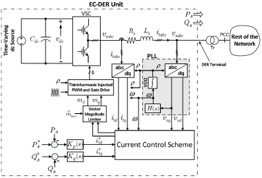
4 1.5 A typical current-mode controlled EC-DER . . . . .

4 1.6 Structure of a conventional PLL . . . .

7 1.7 Performance of the conventional dq-frame-based PLL

during unbalanced magnitude three-phase input

volt-ages . . . .

7 1.8 Performance of the conventional dq-frame-based PLL

during unbalanced magnitude three-phase input

volt-ages . . . .

8 1.9 A typical single-phase PLL scheme . . . .

9 2.1 Representation of Data Samples in a Window . . . .

16 2.2 (a): Real DFT Filter (b): Imaginary DFT Filter . . .

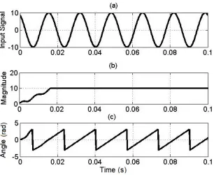
20 2.3 (a): Input signal (b): magnitude (c): rotating angle .

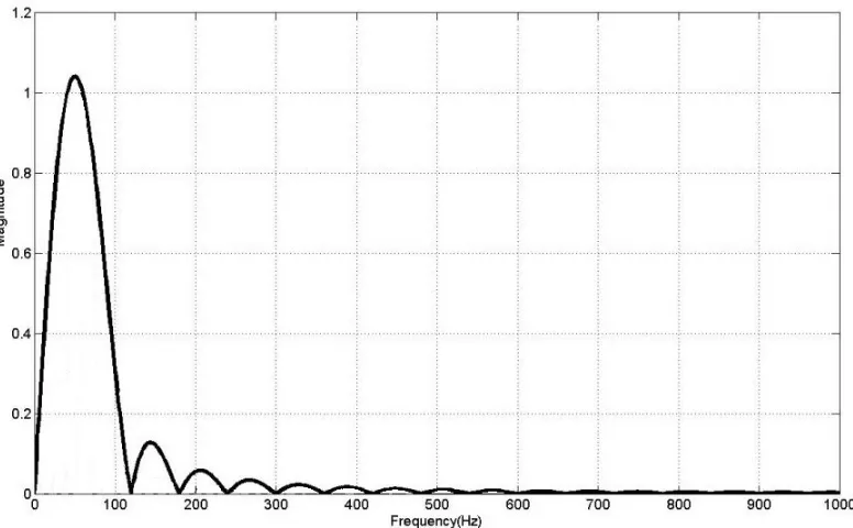
20 2.4 Frequency Response of 1-Cycle DFT’s Real Filter .

21 2.5 Frequency Response of a 1-Cycle DFT’s Imaginary

Filter . . . .

22 2.6 DFT response during nominal frequency operation .

25 2.7 response during o

ff

-nominal frequency operation . .

26 2.8 DFT with di

ff

erent window lengths for AWL technique 27

(10)

2.9 Phase-angle error obtained while phasor

compensa-tion techniques is used in a dynamic frequency

oper-ation test case in the frequency range of 55 to 65Hz .

28 3.1 Magnitude (solid line) and angle (dashdot line) of the

compensation coe

ffi

cients

k

1

and

k

2

as a function of

the frequency . . . .

34 3.2 The ac and dc errors generated in DFT phasor-estimation

for a single-phase system operating under o

ff

-nominal

frequency condition

. . . .

34 3.3 The ac and dc errors generated in phasor estimation

for a three-phase system operating under o

ff

-nominal

frequency condition

. . . .

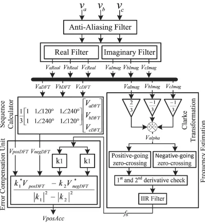
37 3.4 Implementation of the proposed method;

V

xDFT

=

V

xReal

+

jV

xImag

, where

x

=

a

,

b

,

c

, and

V

xReal

is the

real and

V

xImag

is the imaginary part of the DFT

fil-ter’s output . . . .

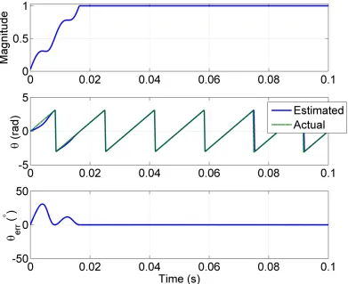
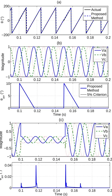
41 3.5 (a): Actual positive-sequence phase-angle versus

es-timated, and (b): phase-angle error for Case 1.a. (c):

phase-angle error for Case 1.b. . . .

44 3.6 Phase-angle error for Case 2 . . . .

45 3.7 Phase-angle error for Case 3 . . . .

46 3.8 Phase-angle error for Case 4 . . . .

47 3.9 Actual and estimated frequency for Case 5 . . . . .

49 3.10Phase-angle error for Case 5 . . . .

49

(11)

3.14Interharmonic test with all of the interharmonics

ap-plied simultaneously as per Table . . . .

51 3.15Results comparison for Case 1.a . . . .

55 3.16Results comparison for Case 1.b . . . .

56 3.17Results comparison for Case 2 . . . .

57 3.18Results comparison for Case 3 . . . .

58 3.19Results comparison for Case 1.a . . . .

59 3.20Results comparison for Case 5 . . . .

60 4.1 The structure of the proposed frequency estimation

technique;

V

esImag

is the imaginary part of the DFT

phasor estimation output . . . .

69 4.2 The phase-angle jump in the

V

_esImag

caused by the

DFT filter length change in comparison to

V

_AccImag

.

70 4.3 Performance comparison of the conventional and

pro-posed frequency estimation techniques

. . . .

71 4.4 Implementation of the proposed method . . . .

72 4.5 Phase-angle error for Case 1, obtained by three

ap-proaches: i) using only AWL, ii) using only phasor

compensation, and iii) the proposed method that is a

mix of both i and ii . . . .

75 4.6 Phase-angle error for Case 2 . . . .

76 4.7 Phase-angle error for Case 3 . . . .

77 4.8 Phase-angle error for Case 4 . . . .

79 4.9 The configuration of the experimental implementation 81

4.10Phase-angle error obtained by the hardware

imple-mentation for Case 1 . . . .

81

(12)

4.12Phase-angle error obtained for Case 3 by: (a)

hard-ware implementation, and (b) simulation results . . .

82 4.13Phase-angle error obtained by hardware

(13)

List of Tables

3.1 Interharmonic Limits for the Evaluation of the

Pro-posed Method [23] . . . .

52 3.2 Results Comparison of IpDFT and the Proposed Method 53

(14)

List of Abbreviations, Symbols, and Nomenclature

AWL: Adaptive Window Length

CVT: Capacitor Voltage Transformer

DFT: Discrete Fourier Transform

EC-DER: Electronically Coupled Distributed Energy Resources

PLL: Phase Locked Loop

SPWM: Sinusoidal Pulse Width Modulation

THD: Total Harmonic Distortion

VCO: Voltage Controlled Oscillator

VSF: Variable Sampling Frequency

(15)

Chapter 1 Introduction

In this chapter, first, an introduction is presented regarding the control systems of the

power-electronic converters that are employed in power-electronically-coupled distributed energy resources

(EC-DERs). Then, the importance of the dq-frame-based controller for the EC-DERs and

its need for a robust and accurate phase-angle-tracking system are described. Thereafter, the

available methods for phase-angle tracking purposes and their specifications are thoroughly

discussed along with the literature survey. Then, the research objectives are defined such that to

introduce a new phase-angle-tracking method with superior performance and fast time response

for three-phase and single phase applications. Finally, the thesis contributions and outline are

presented.

1.1 Control of Power Electronic Converters

In today’s power systems, distributed energy resources (DERs) are scattered throughout a

power system to generate and sometimes absorb electric energy. DERs typically range from

15kW to 10MW and include renewable power generation (e.g., wind and solar), energy

stor-age systems (ESSs), fuel cells, low-head hydro generation, etc. Moving from the conventional

power generation in large power plants to the new types of energy resources and specially the

renewable energy, power electronic converters play an important role to facilitate DERs

(16)

2 Chapter1. Introduction

gration into the grid. This is due to the two major reasons as follows: First, to convert the dc

power produced by dc sources (e.g., solar, battery, and fuel cells) to the ac power to be fed

to the electrical customer or to the grid; second, to obtain more controllability on the output

power and voltage.

The half-bridge voltage source converter (see Figure 1.1) is the fundamental topology

which is used to introduce the voltage source converter (VSC) operation. This converter

con-sists of two bulk capacitors (C₊ and C−) to split the input voltage into half and to provide

the neutral connection. The output voltage equals to Vi/2 or −Vi/2 by turning on the S+ and

S−, respectively. This converter can generate a sinusoidal output voltage at the fundamental

frequency as described in [1]. If the sinusoidal pulse width modulation (SPWM) technique is

employed, low frequency harmonics will not be generated and by using appropriate filters such

as low-pass LC filters at the output of this converter, high frequency components of the voltage

waveform can be filtered out. Thus, the resultant voltage that is seen by the load becomes very

close to the fundamental component. Full-bridge converter (see Figure 1.2) is a variation of the

half-bridge converter. It will provide doubled output voltage magnitude and is recommended

for higher power applications in the single-phase configuration. The concept of the half-bridge

converter can also be extended to three phase applications as can be seen in Figure 1.3.

(17)

1.1. Control ofPowerElectronicConverters 3

Figure 1.2: Full-bridge converter

Figure 1.3: Three-phase two-level full-bridge converter

Half-bridge or full-bridge converters can be controlled by voltage- or current-mode-control

schemes. These schemes can be used depending on the application since each one has its own

strengths and weaknesses. Figures 1.4 and 1.5 show a typical voltage-mode and current-mode

(18)

Figure 1.4: A typical voltage-mode controlled EC-DER

Figure 1.5: A typical current-mode controlled EC-DER

In voltage mode control, the structure of the controller would be simpler. This is because

of the fact that the active and reactive powers are decoupled as discussed earlier, and thus,

(19)

1.1. Control ofPowerElectronicConverters 5

respectively. This can be done by two separate simple controllers. On the other hand, the

current-mode control approach can also be employed to perform the aforementioned control

functions. Although a more complex control system is needed in this case, the current mode

control approach provides some advantages over the voltage-mode control, i.e., the

protec-tion of the EC-DER against over-loading condiprotec-tions and the superior dynamic performance.

Therefore, the current-mode control is a very popular approach in high power applications.

In the current-mode control technique, the converter’s AC side parameters are converted

to direct and quadrature (dq) stationary frame with an abc-to-dq transformation function as

following:            fd fq            =           

cos(ρ) cos(ρ−2π/3) cos(ρ−4π/3)

sin(ρ) sin(ρ−2π/3) sin(ρ−4π/3)

                               fa fb fc                     (1.1)

where fd is the direct- and fq is the quadrature-axis component. This procedure converts the

AC parameters of the grid to their equivalent dq-frame DC parameters. Consequently, the

controller design and implementation become considerably easier. This characteristic has made

the dq-frame transformation very popular in various power system applications [2].

The dq transformation is a function of the angle; thus, a sinusoidal voltage

angle tracking system is required to perform the dq-transformation. Traditionally, a

phase-locked loop (PLL) is employed for this purpose in the structure of the EC-DER control systems

as it is shown in Figure 1.5. The accuracy of this phase-angle tracker directly affects the

performance of the controller, thereby, that of the EC-DER. More importantly, in the presence

of other possible imperfections in the voltage signal(s) of the host network, e.g., harmonic

(20)

1.2 Phase-Angle Tracking Techniques

As discussed in the former section, accurate phase-angle tracking is required in control systems

of power-electronic converters [3]. In particular, under unbalanced and highly distorted grid

conditions, the control performance of the grid-connected voltage-sourced converters depends

on the robustness and accuracy of the estimated phase angle. This is because of the fact that

these conditions adversely affect the PLL performance whose output directly affects the

con-troller and converter performance. A faithful phase-angle-tracking method must rapidly and

accurately obtain the phase angle of the voltage/current signal(s) at the point of connection [4],

[5].

Phase-angle-tracking methods proposed for power-electronic converters can be broadly

cat-egorized into “closed-loop” and “open-loop” methods [6]. In closed-loop methods,

phase-angle of the grid voltage/current is adaptively estimated through a loop mechanism. This loop

is aimed at locking the estimated value of the phase-angle to its actual value. The concept of

PLLs has traditionally been adopted for the purpose of control and operation of power

elec-tronic converters [4], [7]-[9]. In open-loop methods, however, the estimation of the phase-angle

is directly performed through some sort of filtering techniques. The main filtering approaches

include discrete Fourier transform (DFT) [10], [11], weighted least-squares estimation [12],

Kalman filtering [10], [16], and space-vector-based methods [17].

A PLL is generally a closed-loop control system that consists of two major parts: (i) phase

detection and (ii) loop filter. In three-phase power systems, the phase detection module is

nor-mally implemented using the abc-to-dq transformation to obtain two orthogonal components

of the three-phase input signals. Figure 1.6 represents such a PLL. In this figure, the abc-dq

block (i.e., d: direct, and q: quadrature) indicates the phase-detection and the loop filter

con-sists of the compensator, saturation, and voltage-controlled oscillator (VCO) blocks. The loop

filter adjusts the rotational speed of the dq-frame (ω) so that the Vq (i.e., quadrature voltage

component) becomes zero. Then the phase-angle of the three-phase input signals (ρ) is

(21)

1.2. Phase-AngleTrackingTechniques 7

(e.g.,−πtoπ).

Figure 1.6: Structure of a conventional PLL

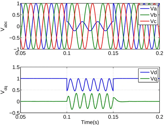
The performance of this PLL is evaluated in Matlab Simulink through an unbalanced

mag-nitude three-phase input voltages (0.2_∠0◦,1_∠−120◦,1_∠−240◦). Figure 1.7 shows the

three-phase input voltages to the PLL and the direct and quadrature voltage components after the

dq-frame transformation. As shown in this figure, a sinusoidal component with doubled grid

0.05 0.1 0.15 0.2

−1 −0.5 0 0.5 1

V abc

0.05 0.1 0.15 0.2

−0.5 0 0.5 1 1.5

Time(s)

V dq

Va Vb Vc

Vd Vq

(22)

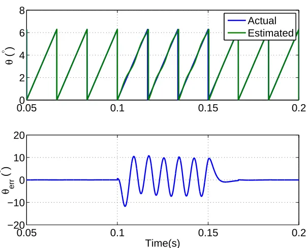
frequency appears after the dq-frame transformation, in both of theVd andVq. Thus, it

gen-erates an error in the estimated phase angle becauseVqis used as the input for the loop filter.

The actual and estimated phase-angles, and the error in the estimated phase-angle are shown in

Figure 1.8.

0.050 0.1 0.15 0.2

2 4 6 8

θ

(

° )

0.05 0.1 0.15 0.2

−20 −10 0 10 20

Time(s)

θ err

(

° )

Actual Estimated

Figure 1.8: Performance of the conventional dq-frame-based PLL during unbalanced magni-tude three-phase input voltages

For the single-phase applications, there is only one sinusoidal signal as the input. Therefore,

the phase-detection structure is modified to generate the orthogonal component of the input

signal by different methods such as using the Park-PLL structure or creating a 90◦ _{delay, etc.}

[13], [14], [15]. However, the time response and/or the accuracy of the PLL would be adversely

(23)

1.2. Phase-AngleTrackingTechniques 9

Figure 1.9: A typical single-phase PLL scheme

The loop filter determines the dynamics of the control system. Therefore, the bandwidth of

the filter is a trade-offbetween the filtering performance and the response time. For example,

the bandwidth of the controller can be tuned in such a way that the harmonics and noise are

eliminated at the cost of a slower response time [4], [18]. Moreover, three-phase PLLs cannot

accurately track the phase-angle under unbalanced conditions. Although decoupling of the

positive- and negative-sequence components have been proposed to deal with this issue

[19]-[21], the proposed solutions do not address the large overshoot associated with the phase-angle

error upon the clearance of the grid fault; further, they still affect the transient response time of

the control loop.

DFT-based techniques are suitable for highly distorted conditions where good filtering

char-acteristics are required [10]; they, however, fail to cope with frequency variations. Two

solu-tions can be considered for this issue as follows: (i) adjustment of the sampling rate to match

the grid frequency and (ii) adapting of the DFT observation window length to match the grid

period. The first solution has been widely used in protection applications. However, variable

sampling rate is not desired in the control system of power-electronic converters since it can

significantly complicate the controller implementation. Moreover, not every system allows

operating at a variable sampling frequency [11]. On the other hand, adaptive observation

win-dow length is appropriate for special applications where a large and fast frequency variation is

experienced [22]. For phase-angle tracking where the frequency deviation is small, large

(24)

observation window length technique.

Several phasor estimation algorithms have been proposed in literature for synchrophasor

applications to achieve higher accuracy under distorted, variable-frequency, and low-frequency

oscillatory conditions [23]. Most of these techniques utilize more than one-cycle observation

window length and require considerably more computation as compared to full-cycle DFT to

achieve higher performance. This makes them less appropriate for the phase-angle tracking in

power-electronic converters.

1.3 Research Objectives

The main objective of the proposed method is to replace the widely used closed-looped PLLs

in power-electronic converters with a new open-loop phasor-based phase-angle-tracking

tech-nique such that it provides better performance and an easier implementation. The proposed

method should be immune to harmonics, noises, voltage imbalances, and grid frequency

vari-ations; in addition, its transient response time should be limited to about one cycle (of the

nominal system frequency), and it does not require any parameter tuning as compared to

PLL-based synchronization methods [4], [7]-[8], [21]. The proposed algorithm should either work

for both single-phase and three-phase applications or two separate algorithms should be

de-vised.

1.4 Contributions

In this thesis, two different approaches are proposed for three- and single-phase applications.

The proposed single-phase method can be simply extended for the three-phase applications

while the proposed three-phase method is only applicable for three-phase applications. In the

proposed three-phase phase-angle-tracking method, the positive-sequence phase-angle needs to

be tracked for the VSC control-system applications. Therefore, a method is developed

(25)

1.4. Contributions 11

in comparison with that of when three separate single-phase PLL units are used.

In the proposed three-phase positive-sequence phase-angle-tracking algorithm, first, the

er-ror in positive-sequence phasor estimated by full-cycle-DFT is calculated analytically. Then,

the accurate positive-sequence phasor is derived based on the two proposed compensation

co-efficients. To further reduce the required processing power, an approximation is proposed to

calculate the compensation coefficients by using Taylor series expansion around the nominal

grid frequency. The aforementioned compensation coefficients are functions of the grid

fre-quency. Therefore, a robust frequency estimation method is also adopted and adjusted for the

purpose of the proposed method as part of the proposed method to accurately track the grid

frequency even during the possible abnormal grid conditions.

In Chapter 4, the single-phase configuration is proposed. In this chapter, it is analytically

presented that the error in the estimated phasor due to the off-nominal frequency operation

is more than that of the three-phase configuration. Accordingly, in addition to the

phasor-compensation, the adaptive-window length (AWL) technique is also suggested for single-phase

applications. It is noted that still fixed sampling rate is being utilized; however, by

imple-menting AWL technique, the calculated accurate phasor becomes completely immune to off

-nominal frequency operation, even beyond the standard limits. Nevertheless, AWL adversely

affects the performance of the frequency estimation method proposed for the three-phase

ap-plications. Hence, a new technique is proposed for the frequency estimation in single-phase

applications. This technique provides very accurate frequency tracking with rapid time

re-sponse. Moreover, it is immune to possible abnormal grid incidents. Later in this chapter, the

proposed method is simulated in Matlab and its performance is evaluated through extensive

study cases. Then, the hardware implementation of the proposed method is done in a digital

(26)

1.5 Thesis Outline

The present thesis consists of five chapters. In the first chapter, an introduction is given to the

conducted research work. Also its contributions to the phase-angle-tracking methods used in

the EC-DER controllers are presented. In the second chapter, the phasor-estimation technique

based on the full-cycle DFT is elaborated. The impact of frequency variation on the DFT-based

phasor estimation and how to cope with them are briefly explained.

In Chapter 3, a new method is proposed for positive-sequence phase-angle tracking of the

three-phase voltage/current signals. First, the error in the estimated positive-sequence phasor

by full-cycle DFT is calculated. Then, this error is compensated using two compensation

coefficients to obtain the accurate phasor. The compensation coefficients are functions of the

grid frequency; therefore, a robust zero-crossing-based frequency-estimation method is also

adopted and adjusted for this purpose. Comprehensive simulation study is conducted using

Matlab to evaluate the performance of the proposed method for almost all of the possible grid

abnormal conditions. The comparison results with the state-of-the-art counterparts are also

included.

In Chapter 4, a phase-angle tracking method is developed for the single-phase applications,

which can be easily extended for the use in three-phase applications. To effectively reduce the

error in the estimated phasor, it is proposed to use AWL along with the phasor compensation

to gain the advantages of both and mitigate the weaknesses of both approaches. The AWL and

phasor compensation are based on the estimated grid frequency. Similar to three phase

appli-cations, a zero-crossing-based frequency-estimation technique is adopted for this purpose. It

is demonstrated that the output of the pre-filtering stage of the frequency-estimation technique

faces undesired transient as DFT window length changes due to the frequency variation. An

enhancement is proposed to effectively eliminate this issue. Extensive simulation studies are

conducted to evaluate the performance of the proposed method during the worst grid conditions

and in compliance with the standards (IEEE Std C37.118.1-2011, IEC 61000-3-6). Finally, the

(27)

1.6. Summary 13

in a real-time DSP.

Chapter 5 summarizes the conducted research. Also, conclusions and the scope of future

works are discussed in this chapter.

1.6 Summary

In the current chapter, an introduction to the EC-DERs and their control systems was

pre-sented. Then, the importance of the phase-angle-tracking within the context of EC-DER’s

control system was discussed. A comprehensive literature survey was presented to cover all of

the state-of-the-art phase-angle-tracking methods, clarifying the advantages and disadvantages

of the different available methods and structures. Then, two research objectives including the

development of a robust and accurate phase-angle-tracking method for three-phase and

single-phase applications were presented. The research objectives were considered to improve the

accuracy and performance of the available methods and to simplify the implementation of the

algorithm. Thereafter, the research contributions were discussed, and the thesis structure was

(28)

Chapter 2 Phasor Estimation

2.1 Introduction

This chapter introduces the conventional phasor estimation technique used in power system

protection and monitoring area. First, the concept of phasor is defined. Then, the windowing

is introduced to picture the time-varient signal analysis in the power systems using phasor

estimation techniques. The DFT phasor estimation technique is discussed in detail, and the

effect of frequency variation on the estimated phasor by DFT is evaluated. Finally, possible

solutions are considered to effectively mitigate or remove the error in the estimated phasor by

DFT, caused by the frequency variation.

2.2 Phasor

The process of extraction of signal parameter (amplitude and phase angle) with respect to

power system frequency is referred to as phasor estimation [35]. Any sinusoidal signalx(t) can

be represented by its phasor form X=A∠θ. A phasor contains the information about the signal

amplitude(A) and phase angle(θ). For example, consider the following signal:

x(t)= Acos(ωt+θ) (2.1)

(29)

2.2. Phasor 15

Equation 2.1 can be rewritten as

x(t)=A.<(ej(ωt+θ)) (2.2)

where<(.) represents the real component of a complex number, and

X= Aejθ = A_∠θ. (2.3)

The phasor for the signal in (2.1) can be represented by (2.3) provided that the signal amplitude

(A), phase angle (θ) and angular frequency(ω) are time invariant. Use of phasor is advantages

as it converts deferential equations to algebraic equations. For example, in case of a series

RL circuit supplied by a sinusoidal source, the differential equation can be expressed in time

domain as

v(t)= Ri(t)+Ldi(t)

dt =Vmcos(ωt) (2.4)

wherev(t) is the voltage signal in the time domain,Ris the resistance andLis the inductance

of the circuit,i(t) is the current signal in the time domain, and theVmis the magnitude if the

sinusoidal voltage signal. If we are only interested in steady-state response of the system, the

differential equation can be converted into an algebraic equation by applying phasor definition

to (2.4). In this case, circuit variables can be calculated simply based on other variables.

V =RI+ jωLI orI = V

R+ jωL orZ = R+ jωL= V

I (2.5)

where,Vis the voltage phasor equals toVm∠θv,Iis the current phasor equals toIm∠θi, andZis

the circuit impedance. Before discussing DFT-based phasor-estimation, it is very important to

understand the concept of ’windowing’ described in the next section.

2.2.1 Windowing

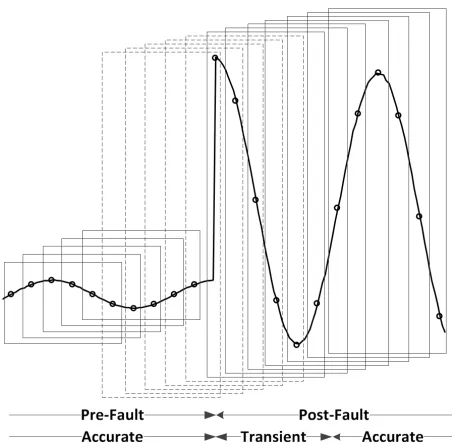
As discussed earlier, for defining the phasor, it has been assumed that the signal is time

(30)

16 Chapter2. PhasorEstimation

Therefore, the phasor estimation is done only for a short span of time which is often termed as

phasor estimation for a window (refer Figure 2.1).

Figure 2.1: Representation of Data Samples in a Window

This short span is generally a power system cycle which is equal to 16.67 ms for a 60 Hz

system. It is assumed that during this period, the signal parameters, i.e., magnitude (A), phase

(θ) and angular frequency (ω) are constant. The data window is continuously updated with

new samples, thereby discarding the previous samples. Thus, phasor estimation is carried out

with every new sample in order to estimate a more accurate phasor. However, the accuracy of

phasors depend upon the accuracy of samples. In the event of any disturbance or fault, these

samples undergo a transition stage which includes samples from both pre-fault and post-fault

instances as shown in Figure 2.1 by the windows with dashed lines. Therefore, in the event of

any fault, there is always a transition time equal to the size of phasor estimation window when

(31)

2.3. DiscreteFourierTransform(DFT) Algorithm 17

2.3 Discrete Fourier Transform (DFT) Algorithm

In practice, power system signals, i.e., measured voltages and currents are often corrupted with

harmonics and noise. In order to accurately estimate the fundamental phasor, it is necessary

to get rid of these extra components contaminating the fundamental signal and extract only

the fundamental frequency component. Various methods have been proposed in literature for

estimating the phasors. However, discrete Fourier transform (DFT) is the most well-known

and applied technique in the area of power system protection and monitoring. The following

section describes the details of phasor estimation based on DFT.

As mentioned in the latter paragraph, DFT is the most commonly and widely used

tech-nique when it comes to protection relays environment. Extraction of a particular frequency

component is done using Fourier transform. However, in relay environment, sampled data at

discrete time steps is available for processing; therefore, the Fourier-transform calculation is

also done in discrete environment and is termed as Discrete Fourier Transform or DFT. Before

defining DFT, let us first understand Discrete-Time Fourier Transform (DTFT).

Equation (2.6) shows the mathematical representation of Fourier transform for a sampled

data signal.

X(jω)=

n=+∞ X

n=−∞

x[n]e−jωn (2.6)

where, ω is 2πf/fs. Generally, a window of sampled data as discussed in the beginning of

this chapter is taken to perform Fourier analysis. Therefore, a truncated version of the above

equation is used for practical purposes. The truncated DTFT is given by (2.7).

XN(jω)= N−1 X

n=0

x[n]e−jωn (2.7)

This truncation is equivalent to multiplying by a rectangular window of data length ’N’ which

results in broadening of spectral peaks and spectral leakage, i.e., the presence of side lobes.

(32)

fs/fn and the frequency of interest is fn. In power system protection, DFT is essentially the

same as DTFT, evaluated at the nominal frequency.

X= 2 N

N−1 X

n=0

x[n]e−j2πfnfsn _(2.8)

KnowingN = fs/fn

X = 2 N

N−1 X

n=0

x[n]e−j2πN fnfnn = 2

N N−1 X

n=0

x[n]e−j2πNn _(2.9)

For a pure sinusoidal signal such asx(t)= Acos(2πfnt+θ)

x[n]= x(n

fs

)= Acos(2πn

N +θ) (2.10)

Equating x[n] into (2.9), one can get (2.11)

X = 2 N

N−1 X

n=0

Acos(2πn

N +θ)e

−j2π_Nn _(2.11)

Using Euler’s identity, (2.11) can be rewritten as (2.12).

X = 1 N

N−1 X

n=0

Aej(2πNn+θ)+e−j(2π n N+θ)

e−j2πnN (2.12)

Simplifying (2.12) results into (2.13) which can further be simplified into (2.14).

X = 1 N

N−1 X

n=0

Aejθ+e−j(4πNn+θ) (2.13)

X = Aejθ+ Ae −jθ N

N−1 X

n=0

e−j4πNn (2.14)

Assumingr = e−j4πN1 of a Geometric progression (GP) series, the sum of a finite GP series is

given by (2.15).

N−1 X

n=0

rn= 1+r+r2+· · ·+rN−1 = 1−r N

(33)

Simplifying (2.14) using (2.15), we obtain

N−1 X

n=0

e−j4πNn = 1−e

−j4πN_N

1−e−j4π_N1 =0 (2.16)

Therefore, (2.14) becomes

X(fn)= Ae jθ ₌

A_∠θ (2.17)

Equation (2.17) represents phasor for any sinusoidal signal with the fundamental frequency of

fn. Thus,

X(fn)=

2

N N−1 X

n=0

Acos(2πn

N +θ)e

−j2π_Nn _(2.18)

Using (2.10) and equating into (2.18), we obtain (2.19)

X(fn)=

2

N N−1 X

n=0

x[n]e−j2πNn = 2

N N−1 X

n=0

x[n] cos 2πn

N

| {z }

Xr:Real Filter

+j 2 N

N−1 X

n=0

−x[n] sin 2πn

N

| {z }

Xi:Imaginary Filter

(2.19)

Xr = Real Filter=

2

N cos(

2π

Nn) (2.20)

Xi =Imaginary Filter= −

2

N sin(

2π

Nn) (2.21)

wheren= 0, ...,N−1.

Phasor’s amplitude and angle can be computed by (2.22) and (2.23), respectively. In power

system protection area, it is very common to split the complex exponential term of DFT into

real and imaginary filters as shown in (2.20) and (2.21).

A= p(Xr)2+(Xi)2 (2.22)

(34)

Figure 2.2: (a): Real DFT Filter (b): Imaginary DFT Filter

Figure 2.2 shows the real and imaginary filters for a 64 sample per cycle and 60 Hz power

system, represented by (2.20) and (2.21).

(35)

x(t)= 10.cos(2π.60.t+π/6) (2.24)

Equation (2.24), represents a pure sinusoidal 60 Hz signal. Figure 2.3 (a) shows the input

signal. When the input signal is passed through DFT filters, it returns the magnitude and angle

as represented by Figure 2.3 (b) and (c). It can be observed from time response that DFT has

a transient time of 1-cycle. Also, it gives a constant phasor magnitude output for a pure 60 Hz

signal once the transient time is over. It can also be observed from the angle that it is constantly

varying. As the window of samples are updated upon acquisition of a new sample, the inherent

phase shift 2π/N occurs. Because of this phenomenon, the phasor obtained using this method

is called rotatory phasor. The estimated phasor’s phase angle is very similar to the output of

the PLL as the estimated phasor rotates in the complex plane, while the DFT sampling window

is being shifted in time.

Figure 2.4: Frequency Response of 1-Cycle DFT’s Real Filter

In Figure 2.4 and Figure 2.5, the frequency response of a 1-cycle DFT of real and imaginary

filters is shown. It can be observed from the real and imaginary filter’s frequency response

(magnitude) of a 1-cycle DFT that it removes DC and integer harmonics, suppresses noise, and

(36)

Figure 2.5: Frequency Response of a 1-Cycle DFT’s Imaginary Filter

2.4 Decaying DC and CVT Transient Filters

The DFT phasor estimation technique can be used for both voltage and current signals. In

case of using current signals, the additional decaying dc component generated during the fault

can be attenuated or removed by utilizing the numerical compensation technique proposed

in [31]. In case, the voltages measured by capacitor voltage transformers (CVTs) are used,

additional CVT transient filters, such as the one presented in [32] should be applied to

three-phase voltage signals before the phasor estimation. If any filter is employed before phasor

estimation, phase-angle should be accordingly shifted to compensate for the delay of the filter

at the grid frequency.

2.5 Frequency Variation

If the period of the input signal is equal to the DFT window length, during the steady-state

(37)

2.5. FrequencyVariation 23

grid-frequency fluctuates from its nominal value, the estimated phasor by the DFT would be

imperfect. In this case, the DFT window length can be changed so that it include more or less

samples to fit the DFT window length to the period of the input signal. Thus, the error in the

es-timated phasor by the DFT can be reduced. This is an example on how to make the DFT phasor

estimation adaptive to the grid frequency variations, and off-nominal frequency of operation.

The variable sampling frequency is another method to overcome the aforementioned problem

although its implementation is more complex than the variable window length. All of these

techniques are based on the estimated grid frequency; therefore, a robust frequency-estimation

method is inevitable for these techniques to effectively reduce the error in the estimated phasor.

DFT-based phasor-estimation is not immune to frequency variations in the input signal by

itself. However, by using techniques such as adaptive window length (AWL), variable

sam-pling frequency (VSF), and phasor compensation, the error in the estimated phasor by DFT is

prevented or compensated. AWL is a technique to change the length of the DFT filters such

that they match the period of the input signal. Thus, the AWL makes the DFT algorithm

adap-tive to the frequency variations in the input signal. The accuracy of AWL mainly depends

on the sampling resolution. Therefore, to decrease the phasor estimation error with this

tech-nique, higher sampling frequency would be required. The AWL can be useful in applications

that require wide frequency variation range and less accuracy, e.g., fast bus transfer

applica-tions. VSF, however, keeps the number of samples in the DFT filters constant, and adjusts

the sampling frequency to match the DFT window length with the period of the fundamental

frequency component. The VSF is useful where a narrow range of changes of frequency but a

higher accuracy is expected. As such, VSF is the most popular technique used in the protection

relays.

Another approach to make the DFT adaptive to the frequency variation is phasor

compen-sation. This can be done by calculating the error caused by the off-nominal frequency operation

in the DFT phasor-estimation and then, to compensate the imperfect phasor to obtain the

(38)

coefficients. The advantage of this method is the simplicity of implementation because it does

not require any hardware modifications and it adds negligible calculation burden to the

con-ventional DFT. Nevertheless, by compensating the error that is caused by the fundamental

frequency component while the signal is contaminated with harmonics during the off-nominal

frequency operation, the errors caused by harmonics appear in the estimated phasor. This is

due to the fact that full cycle DFT filters tuned to the nominal frequency do not fully eliminate

harmonics during off-nominal frequency operation. This error increases by deviating from the

fundamental frequency. Therefore, phasor compensation is not recommended if higher

accu-racy is needed during considerable off-nominal frequency operation with distorted signals.

2.5.1 O

ff

-Nominal Frequency Operation with Conventional DFT

To study the performance of the conventional DFT phasor estimation technique during off

-nominal frequency variation, a simulation is done as follows. First a 60Hz DFT is considered,

whose window length is equal to the period of a 60Hz sinusoidal signal. Then, two signals

with unit magnitudes, one with 60Hz frequency and the other with 55Hz are applied to the

DFT input. As it is shown in Figure 2.6, the 60Hz DFT accurately estimates the input signal’s

magnitude and phase-angle. It is demonstrated that after the one-cycle transient response of

(39)

Figure 2.6: DFT response during nominal frequency operation

For the 55Hz signal, however, the estimated phasor by the 60Hz DFT will be imperfect both

in magnitude and phase-angle. This is shown in Figure 2.7. Although the error in magnitude

is not very high, the error in the phase-angle is considerable. Therefore, in order to use the

conventional DFT as a phase-angle tracking method, this error needs to be effectively reduced

(40)

Figure 2.7: response during off-nominal frequency operation

2.5.2 Adaptive Window Length and Phasor Compensation

Since phasor estimation based on fixed sampling frequency is of interest for the control-system

applications of the EC-DERs, AWL and phasor compensation are discussed in this subsection.

The advantage of AWL is its simple implementation because it is based on the fixed sampling

rate. Figure 2.8 shows that how a DFT filter length can be changed so that it matches the period

of the input signal. However, there is still a small discrepancy between the DFT window length

and the period of the input signal. For example, if the grid frequency is 57Hz, the number

of samples can be calculated by dividing the sampling frequency by the grid frequency, i.e.,

64×60/57 = 67.37. By choosing the closest integer number to 67.37, i.e., 67, a discrepancy

(41)

the DFT window length can only be changed in discrete steps, i.e., a sample long in the length.

As it is proposed in this thesis in Chapter 4, the error in the phasor caused by this discrepancy

can be compensated using the phasor-compensation.

Figure 2.8: DFT with different window lengths for AWL technique

If the phasor compensation is used, the error in the estimated phasor increases by deviating

from the nominal frequency while the signal is distorted with harmonics (see Figure 2.9). This

is because of the fact that the errors caused by harmonics during off-nominal frequency of

operation are not compensated through the phasor compensation. However, it is proposed

in Chapter 4 to use AWL along with the phasor compensation. Consequently, the deviation

between the fundamental frequency of the DFT phasor-estimation and the actual signal’s is

kept below 0.5Hz. This guarantees that the error caused by harmonics in phasor compensation

(42)

0.5

1

1.5

2

2.4

0

0.2

0.4

0.6 θ

err

(

°

)

Phasor Compensation

(b)

Figure 2.9: Phase-angle error obtained while phasor compensation techniques is used in a dynamic frequency operation test case in the frequency range of 55 to 65Hz

2.6 Summary

In this chapter, first the concept of phasor estimation and its application in power system

pro-tection was introduced. The importance of accurate phasor estimation was then discussed. The

chapter also explained the process of windowing which enables phasor estimation by

calcu-lating the phasor upon the arrival of every new sample. The chapter then discussed the DFT

phasor estimation and the effects of off-nominal frequency operation. It was shown that the

DFT phasor-estimation is not immune to frequency variations, and thus, three methods were

investigated to add the frequency adaptation capability to DFT phasor-estimation technique as

follows: i) AWL, which changes the DFT window length to match with the signal’s period,

ii) VSF that changes the sampling frequency to adjust the DFT window length with the

in-put signal’s period, and iii) the phasor compensation to compensate the error caused by the

off-nominal frequency operation in the estimated phasor by DFT. It is discussed that the fixed

sampling frequency is of interest to be used in the control systems of the EC-DERs. Thus, it

was proposed to use AWL with phasor compensation to obtain an accurate DFT-based phasor

(43)

Chapter 3 Positive-Sequence Phase-Angle Tracking

3.1 Introduction

In this chapter, a positive-sequence phase-angle tracking method is proposed for three-phase

applications. Although the proposed method is elaborated for voltage signals, it can also be

applied to current signals, e.g., for series-connected converters. In Section 3.2, the DFT error

associated with the calculation of the positive-sequence phasor in a variable-frequency

envi-ronment is accurately formulated. Then, the accurate phase-angle is calculated based on the

estimated positive- and negative-sequence of the voltage phasors, estimated frequency, and

two proposed compensation coefficients. Moreover, a simple approximation is proposed to

reduce the processing power required to compute two compensation coefficients. In Section

3.3, five comprehensive case studies are conducted in the Matlab software environment to

eval-uate the performance of the proposed method. Although it is not common to test the

phase-angle-estimation methods towards interharmonics, comprehensive interharmonic tests are also

conducted in this chapter. Finally, the conclusions and comparison with the state-of-the-art

methods are presented in Section 3.5.

(44)

30 Chapter3. Positive-SequencePhase-AngleTracking

3.2 Proposed Phasor Measurement Algorithm

3.2.1 Phase-Angle Measurement of Positive-Sequence Components using

Standard DFT

To determine the DFT error for positive-sequence phasor estimation under off-nominal

fre-quency operation, let us consider the phasor of a voltage signal estimated by a full-cycle DFT.

Equation (3.1) represents a given voltage signal in a discrete-time domain.

v[n]=Vmcos

2πfg N fn

n+θ0 !

(3.1)

wherev[n] is the discrete form of a continuous-time signal sampled at the rate ofNsamples per

fundamental-component cycle, andnspecifies the sample number. Vmis the signal magnitude,

and θ0 denotes the angle at n = 0. The grid actual and nominal frequencies are fg and fn,

respectively. According to the definition of full-cycle DFT, the fundamental-frequency phasor

(V) of a discrete voltage signalv[n] can be represented as

V = 2 N

N−1 X

n=0

v[n]e−j2Nπn. (3.2)

If the grid frequency fgequals the nominal frequency fn, the voltage phasor ofv[n] is calculated

as V = Vmejθ0 = Vm∠θ0. However, if the grid frequency deviates from its nominal value,

the phasor estimation using standard DFT is inaccurate. Assuming that the grid frequency is

known but different from the nominal frequency, the fundamental-frequency phasor ofv[n] can

be written as

Ves=

2

N N−1 X

n=0

Vmcos (

2π

N fg fn

n+θ0)e−j

2π

Nn (3.3)

whereVesis the estimated voltage-phasor using full-cycle DFT. In a full-cycle DFT algorithm,

acquisition of a new sample is equivalent to forward shifting of the signal samples in time

(45)

3.2. ProposedPhasorMeasurementAlgorithm 31

is captured. In other words, the estimated voltage/current phasor rotates counter clockwise as

new samples arrive. Equation (3.3) can be simplified to (3.9) by expanding cosine function to

the summation of complex exponential functions from Euler’s formula, and then determining

the result of the summation by using geometric series as follows.

Ves= Vm

N N−1 X

n=0

ejθ0_ej2Nπ( fg

fn−1)n+_e−jθ0_e−j2Nπ( fg fn+1)n

.

Now let us definer1andr2as

r1 =e

j2_Nπ(fg_fn−1)_,

r2 =e

−j2_Nπ(fg_fn+1)

(3.4)

so that (3.4) can be rewritten as

Ves= Vm

N e jθ0

N−1 X

n=0

r₁n+ Vm N e

−jθ0

N−1 X

n=0

r₂n. (3.5)

Using (3.6), the summations in (3.5) are expanded and simplified as in (3.7) and (3.8).

1+r+r2+...+rN−1= 1−r

N

1−r (3.6)

N−1 X

n=0

r₁n= r0₁+r₁1+...+rN−1₁ = 1−e j2π(fg_{f n})

1−ej2Nπ( fg fn−1)

(3.7)

N−1 X

n=0

r₂n =r0₂+r₂1+...+rN−1₂ = 1−e −j2π(fg_fn)

1−e−j2Nπ( fg fn+1)

(3.8)

Equation (3.9) is obtained by reinserting (3.7) and (3.8) into (3.5).

Ves = Vm

N e

jθ0 1−e

j2π(_{f n}fg)

1−ej2Nπ( fg fn−1)

+ Vm N e

−jθ0 1−e

−j2π(fg_fn)

1−e−j2Nπ( fg fn+1)

. (3.9)

The estimated phase-angle of (3.3) is based on the assumption that the time reference is at

(46)

the real-time phase-angle of the voltage waveform is needed to be measured. Thus, we would

like to determine the phase-angle of the measured signal at the last acquired sample, i.e., at the

present time. According to (3.1), the phase-angle at the last acquired sample, i.e., n = N −1

can be specified as

θN−1 = 2π fg fn

1− 1

N !

+θ0 (3.10)

where θN−1 is the phase-angle of the voltage signal considering the time of the last sample

acquisition as the reference time. Similarly, the phasor of the voltage signal considering the

last sample acquisition as the reference time can be calculated. This phasor is referred to as the

accurate phasorVAcc, and given by

VAcc =Vme j

2πfg_fn(1−_N1)+θ0

. (3.11)

Since it is required to track the angle of the accurate phasor for phase-angle-tracking

applica-tions, the estimated phasor in (3.9) needs to be written in terms of VAcc. In reference to the

terms in (3.9), for the sake of simplification it is better to write this equation in terms ofVAcc

and V_Acc∗ , where ’∗_{’ denotes the complex conjugate. Therefore, the first and second terms in}

the right hand side of (3.9) are multiplied with and divided by exp(j(2πfg/fn(1−1/N))) and

exp(−j(2πfg/fn(1−1/N))), respectively as below.

Ves= Vm

N e jθ0e

j

2πfg_fn₍1−1

N)

ej

2πfg_fn₍1−1

N)

1−ej2πfgf n 1−ej

2π N _fg fn−1 + Vm N e

−jθ0e

−j

2πfg_fn₍1−1

N)

e−j

2πfg_fn₍1−1

N)

1−e−j2πfgfn

1−e−j

2π N

_fg

fn+1

(3.12)

By extractingVAccandV_Acc∗ as per (3.11), (3.12) can be written as

Ves= VAcc

1

N e−j

2πfg_fn(1−_N1)

1−ej2πfgfn

1−ej

2π N _fg fn−1 +V ∗ Acc 1 N ej

2πfg_fn(1−_N1)

1−e−j2πfgfn

1−e−j

2π

N

_fg

fn+1

(47)

= VAcc

1

N

e−j2πfgfn ₋₁

e−j2πN fnfg ₋_e−j2Nπ

+V ∗ Acc 1 N

ej2πfgfn ₋₁

ej2πN fnfg ₋_e−j2Nπ

=VAcc

1

N

e−jπfgfn

e−jπfgfn ₋_ejπ fg fn

e−j2_Nπ_ejNπ

1−fg_fn

ej

π

N

1−fg_fn

−e−j

π

N

1−fg_fn

!+V

∗ Acc

1

N

ejπfgfn

ejπfgfn ₋_e−jπ fg fn

e−j2_Nπ_ejNπ

1+fg_fn

ej

π

N

1+fg_fn

−e−j

π

N

1+fg_fn

!

=VAcc

sinπfg

fn

Nsin_Nπ fg

fn −1

e jπ

fg fn(

1−N

N )+

1 N

| {z } k1

+V∗ Acc

sinπfg

fn

Nsin_Nπ fg

fn +1

e jπ

fg fn(

N−1

N )+

1 N

| {z } k2

. (3.13)

Thus, the estimated phasor can be written in terms ofVAccand its complex conjugateVAcc∗ as in

Ves= k1VAcc+k2VAcc∗ . (3.14)

In (3.14),k1andk2are defined as follows:

k1 =k1Mag∠k1Ang, k2 =k2Mag∠k2Ang (3.15)

in which,

k1Mag =

1

N

sinπfg

fn −1

sin_Nπ fg

fn −1

, k1Ang = π

1−N

N ! fg fn +1 ! (3.16)

k2Mag =

1

N

sinπfg

fn +1

sin_Nπ fg

fn +1

, k2Ang =π

N−1

N ! fg fn −1 ! . (3.17)

Equation (3.14) shows that the estimated phasor has a linear relationship with the accurate

phasor and its complex conjugate for a given grid frequency. In this equation,k1 andk2are the

compensation coefficients. It is noted that the compensation coefficients are neither sensitive

to the signal magnitude nor to the angle. Further, they are time invariant and are only functions

of the grid frequency. Magnitude and angle of k1 andk2 for a frequency range of 55Hz to 65

(48)

deviates 1.14% by a 5-Hz frequency deviation. Further, the relationship ofk1magnitude with

frequency is very similar to a quadratic function. Figure 3.1 also illustrates that the magnitude

of k2 is very close to zero and deviates 4.3% by a 5-Hz frequency deviation. Besides, the

relationship ofk2magnitude with frequency is very similar to a linear function. As depicted in

Figure 3.1, the angles ofk1andk2, have linear relationships with the grid frequency.

55 60 65

0.988 0.994 1

Frequency (Hz)

Magnitude

k 1

55 60 65−10

5 20

Angle

55 60 65

−0.05 0 0.05

Frequency (Hz)

Magnitude

k 2

55 60 65−15

0 15

Angle

Figure 3.1: Magnitude (solid line) and angle (dashdot line) of the compensation coefficientsk1

andk2 as a function of the frequency

Figure 3.2: The ac and dc errors generated in DFT phasor-estimation for a single-phase system

operating under off-nominal frequency condition

Equation (3.14) also shows that, for a given off-nominal frequency, the error in the phasor

estimation has two components. The first component of the error is generated due to the

com-plex factork1which scales the magnitude and shifts the angle of the accurate phasor,VAcc. The

(49)

is, hereinafter, referred to as the “dc error”. The second component of the error, however, is

generated through the scaling of the magnitude and shifting the angle of the accurate phasor

conjugate, V_Acc∗ . Since V_Acc∗ rotates clockwise, the error generated by this component has a

sinusoidal shape whose frequency is twice of the grid frequency; thus, it is called “ac error”

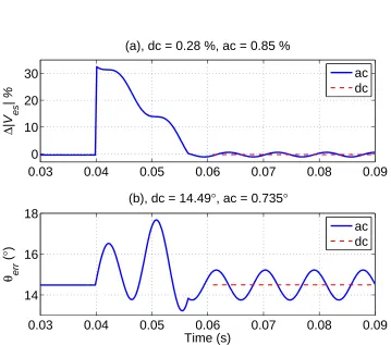
in this thesis. This fact is illustrated in Figs. 3.2.(a) and (b), where the magnitude (∆|Ves|)

and phase-angle errors (θerr) of a 57-Hz sinusoidal signal are indicated, respectively. As it is

shown, the errors have both dc and ac components. For a 57-Hz sinusoidal signal, the error in

magnitude is only 0.4% dc and 2.55% peak ac; however, the error in phasor angle is 14.49◦

dc and 1.47◦peak ac, which are considerable. Equation (3.14) can separately be reiterated for

each phase of a three-phase system as

VaDFT = k1VaAcc+k2VaAcc∗ (3.18)

VbDFT = k1VbAcc+k2VbAcc∗ (3.19)

VcDFT = k1VcAcc+k2VcAcc∗ (3.20)

whereVaAcc, VbAcc, andVcAcc are the three-phase accurate voltage phasors, andVaDFT, VbDFT,

andVcDFT are the estimated phasors of three-phase voltages obtained by full-cycle DFT.

Ap-plying the Fortescue’s transform, the positive-sequence voltage phasor is obtained as

VposDFT = 1₃(VaDFT +αVbDFT +α2VcDFT) = 1

3k1(VaAcc+αVbAcc+α

2_V

cAcc) + 1

3k2(VaAcc+α

2_V

bAcc+αVcAcc)∗

= k1VposAcc+k2VnegAcc∗ (3.21)

whereα=1_∠120◦_,_V

posDFT is the positive sequence of the estimated voltage phasors,VposAccis

the positive sequence of accurate voltage phasors, andV_negAcc∗ is the complex conjugate of the

(50)

phasor estimation, the error of the estimated positive-sequence phasor has two components.

The first component generates dc error, while the second component generates ac error. Figure

3.3 shows the error in magnitude and angle of the estimated positive-sequence phasor for a

57-Hz three-phase sinusoidal signal. The three-phase voltages are balanced until t = 0.04

s and, then, phase-C voltage is forced to zero to simulate a severe single-phase-to-ground

fault. As it is shown in the figure, the ac component of errors in both magnitude and

phase-angle is zero before the fault occurrence. This is due to the fact that the three-phase voltage

is balanced and, thus, there is no negative-sequence component. Once the fault takes place,

the negative-sequence component significantly increases; hence, the ac error of the estimated

positive-sequence phasor is expected to grow. As illustrated in Figure 3.3, once DFT transient

disappears, i.e., at t = 0.04 + 0.0167 = 0.0567s, the error in magnitude is 0.28% dc and

0.85% ac peak, while the angle error is 14.49◦_{dc and 0.735}◦ _{ac peak. It is evident that the dc}

component of the phase-angle error is significant, while its ac component is quite negligible,

even during a solid close-in single-phase-to-ground fault. Similar approach to the one adopted

in (3.21) can be employed to determine the negative-sequence component of the estimated

voltage phasors as

VnegDFT =k1VnegAcc+k2VposAcc∗ (3.22)

where VnegDFT is the negative sequence of the estimated phasors, VnegAcc is the negative

se-quence of the accurate voltage phasors, and V_posAcc∗ is the complex conjugate of the positive

sequence of the accurate voltage phasors. Assuming k1 and k2 are known and solving for

(3.21) and (3.22),VposAcc can be calculated as

VposAcc =

k∗₁VposDFT −k2VnegDFT∗ |k1|2− |k2|2

. (3.23)

The recent equation is the base of the proposed algorithm for accurate phase-angle tracking

(51)

though the focus of the proposed method is on the phase-angle, it also accurately tracks the

positive-sequence voltage magnitude and the frequency as by-products.

As discussed earlier, VnegAcc is zero if the three-phase system is operating under balanced

condition. Under normal-running condition, where there is no fault impacting the network,

the negative-sequence voltage is very small (<2%) [27]; thus, the ac error is negligible. If

the negative-sequence component is ignored in (3.23), VposAcc can be approximated by the

following equation, which again reduces the required processing power. This equation can be

used if the accuracy of the algorithm during the unbalanced-voltage operating conditions is not

a necessity.

VposAcc =

VposDFT k1

. (3.24)

0.03 0.04 0.05 0.06 0.07 0.08 0.09 0

10 20 30

∆

|V

es

| %

(a), dc = 0.28 %, ac = 0.85 %

ac dc

0.03 0.04 0.05 0.06 0.07 0.08 0.09 14

16 18

Time (s)

θ err

(

°

)

(b), dc = 14.49°, ac = 0.735°

ac dc

Figure 3.3: The ac and dc errors generated in phasor estimation for a three-phase system

8-19-2014 12:00 AM A Phase-Angle Tracking Method for Synchronization of Single- and Three-Phase Grid-Connected Converters

Scholarship@Western

Scholarship@Western

A Phase-Angle Tracking Method for Synchronization of Single-

A Phase-Angle Tracking Method for Synchronization of Single-

and Three-Phase Grid-Connected Converters

and Three-Phase Grid-Connected Converters

A PHASE-ANGLE TRACKING METHOD FOR SYNCHRONIZATION OF

SINGLE- AND THREE-PHASE GRID-CONNECTED CONVERTERS

(Thesis format: Monograph)

by

Farzam Baradarani

Graduate Program in Electrical and Computer Engineering

A thesis submitted in partial fulfillment

of the requirements for the degree of

Masters in Engineering Sciences

The School of Graduate and Postdoctoral Studies

The University of Western Ontario

London, Ontario, Canada

c

Abstract

Acknowledgement

Dedication

To my brother, ’Aryaz’.

Contents

Abstract

ii

Acknowlegements

iv

Dedication

v

List of Figures

viii

List of Tables

xii

List of Abbreviations, Symbols, and Nomenclature

xiii

List of Abbreviations, Symbols, and Nomenclature

xiii

1 Introduction

1

1.1 Control of Power Electronic Converters . . . .

1

1.2 Phase-Angle Tracking Techniques . . . .

6

1.3 Research Objectives . . . .

10

1.4 Contributions . . . .

10

1.5 Thesis Outline . . . .

12

1.6 Summary . . . .

13

2 Phasor Estimation

14

2.1 Introduction

. . . .

14

2.2 Phasor

. . . .

14

2.2.1 Windowing . . . .

15

2.3 Discrete Fourier Transform (DFT) Algorithm . . . .

17

2.4 Decaying DC and CVT Transient Filters

. . . .

22

2.5 Frequency Variation . . . .

22

2.5.1 O

ff

-Nominal Frequency Operation with

Con-ventional DFT

. . . .

24

2.5.2 Adaptive Window Length and Phasor

Compen-sation . . . .

26

2.6 Summary . . . .