1267 |
P a g e
Burr Type III Software Reliability Assessment Using
SPC-An Order Statistics Approach
K.Sobhana
1,Dr. R. Satya Prasad
2,Dr.R.Kiran Kumar
3Research Scholar, Department of Computer Science, Krishna University, Machilipatnam,
Andhra Pradesh ( India)
Associate Professor, Dept. of Computer Science & Engg., Acharya Nagarjuna University,
Guntur, Andhra Pradesh (India)
Assistant Professor ,Department Of Computer Science, Krishna University, Machilipatnam,
Andhra Pradesh (India)
ABSTRACT
Assessment of Software Reliability is a vital aspect to be considered during the software development process.
Software reliability is the probability that given software functions work without failure in a specific
environment during a specified time. It can be assessed using Statistical Process Control(SPC). SPC is a method
of quality control that uses statistical methods to control and monitor a software process and thereby contributes
significantly to the improvement of software reliability. Control charts are widely used SPC Tools to monitor
software quality. The proposed model involves estimation of the parameters of the mean value function and
hence these values are used to develop the control charts. The Maximum Likelihood Estimation (MLE) method
is used to derive the estimators of the distribution. In this paper we propose a mechanism to monitor software
quality based on order statistics of cumulative observations of time domain failure data using mean value
function of Burr type III distribution based on Non-Homogeneous Poisson Process.
Keywords- Burr Distribution, ,Control Charts, Mean Value Function, Non-Homogeneous Poisson Process,
Order Statistics, Probability Limits, Software Reliability, Statistical Process Control.
I. INTRODUCTION
Software reliability is one of the most important characteristics of software quality. Reliable software systems
can be produced and maintained by employing quality measurement and management technologies during the
software life cycle. Software Reliability is the probability of failure free operation of software in a specified
environment during specified time[1].
The monitoring of Software reliability process is a far from simple activity. In recent years, several authors
have recommended the use of SPC for software process monitoring. A few others have highlighted the potential
pitfalls in its use[2].
The main thrust of the paper is to formalize and present an array of guidelines in a disciplined process with a
view to helping the practitioner in putting SPC to correct use during software process monitoring.
Over the years, SPC has come to be widely used among others, in manufacturing industries for the purpose of
controlling and improving processes. Our effort is to apply SPC techniques in the software development process
1268 |
P a g e
several processes for software development, including software reliability process. SPC is traditionally so well
adopted in manufacturing industry. In general software development activities are more process centric than
product centric which makes it difficult to apply SPC in a straight forward manner.
The utilization of SPC for software reliability has been the subject of study of several researchers. A few of
these studies are based on reliability process improvement models. They turn the search light on SPC as a means
of accomplishing high process maturities. Some of the studies furnish guidelines in the use of SPC by modifying
general SPC principles to suit the special requirements of software development [3] (Burr and Owen[4]; Flora
and Carleton[5]). It is especially noteworthy that Burr and Owen provide seminal guidelines by delineating the
techniques currently in vogue for managing and controlling the reliability of software. Significantly, in doing so,
their focus is on control charts as efficient and appropriate SPC tools.
It is accepted on all hands that Statistical process control acts as a powerful tool for bringing about improvement
of quality as well as productivity of any manufacturing procedure and is particularly relevant to software
development also. Viewed in this light, SPC is a method of process management through application of
statistical analysis, which involves and includes the defining, measuring, controlling, and improving of the
processes[6].
II. PROPOSED WORK
A.BURR Type III NHPP Model
NHPP software reliability growth models have been proposed to assess the reliability of software [13].In these
models ,the number of software failures display the behavior of non-homogenous PoissonProcess[20].These
models consider the debugging process as a counting process characterized by its mean value function. Software
reliability can be estimated once the mean value function is determined. Model parameters are usually estimated
using Maximum Likelihood method or Genetic Algorithms.
The various notations used in NHPP model are :
{N(t),t>0} represents the cumulative number of failures by time „t‟.
m(t) denotes the expected number of software failures by time „t‟.
„a‟ represents the expected number of software failures eventually detected. „b‟ denotes the failure detection rate.
λ (t) corresponds to intensity function of software failures [9,13,23].
The Assumptions of NHPP Model are :
1.A Software system is subject to failures during execution caused by faults remaining in the system.
2.All faults are mutually independent from a failure detection point of view.
3.Failure rate of the software depends on the faults remaining in the system.
4.The number of faults detected at any time is proportional to the remaining number of faults in the software.
Since the expected number of errors remaining in the system at any time is finite, m(t) is bounded,
non-decreasing function of „t‟ with the boundary conditions
m(t) =
t
a
t
,
0
,
0
1269 |
P a g e
The behaviour of software failure phenomena can be illustrated through N(t) process. Several time domain
models exist in the literature which specify that the mean value function m(t) will be varied for each NHPP
process.
In this paper we consider the mean value function of Burr Type III software reliability growth model as
m
(
t
)
a
[
1
t
c]
b (1)Here, we consider the performance given by the Burr Type III software reliability growth model based on order
statistics and whose mean value function is given by
i c b
t
m
a
t
r
)
(
1
)( (2)
Where [m(t)/a] is the cumulative distribution function of Ordered Burr distribution model
This is considered as Poisson model `with mean a. Let Sk be the time between (k-1) th
and kth failure of the
software product. It is assumed that Xk be the time up to the kth failure. We need to find out the probability of
the time between (k-1)th and kth failures. The Software Reliability function is given by
R= [ ( ) ()] )
1 (
)
/
(
X mx s msk
k
s
e
X
S
(3)B. Parameter Estimation Based on Inter Failure Times The mean value function of Order Burr Type III is given by
r b c it
a
t
m
(
)
1
(
)
(4)The constants a, b and c in the mean value function are called parameters of the proposed model. To assess the
software reliability, it is necessary to compute the expressions for finding the values of a, b and c. For doing
this, Maximum Likelihood estimation is used whose Log Likelihood function is given by
LLF = i r n r
n
i
t
m
t
Log
[
(
)
(
)
1
(5)Differentiating m(t) with respect to „t‟ we get
(t)
(t) = ( 1) ( 1)]
)
(
1
[
*
)
(
t
i c
ti
c brrabc
(6) ! ) ( } ) ( { ) ( n e t m n t N P t m n nlim
! } ) ( { n e a n t N P a n
0
,
1
,
2
...
1270 |
P a g e
The log likelihood equation to estimate the unknown parameters a, b, c after substituting (4) in (5) is given by
LogL= -[a[1+(tn)-c]-b]r+
n i c b a r 1 ] log log log [log +
n i i ci c t
t br 1 )] log( ) 1 ( ) ) ( 1 log( ) 1 (
[ (7)
Differentiating LogL with respect to „a‟ and equating to 0 (i.e
log
0
)
a
L
we get
ar =
r
t
n
(
1
(
n)
c)
br
(8)
Differentiating LogL with respect to „b‟ and equating to 0 (i.e
log
0
)
b
L
we get
g(b) = log(1 ( ) ) (1 ( ) ) log(1 ( )1) 1 2 1 1
n br nn i i t r t n t r b n (9)
Again Differentiating g(b) with respect to „b‟ and equating to 0 (i.e
log
20
)
2
b
L
g'(b) =
2
2(
1
(
)
1)
.
log
2(
1
(
n)
1)
br n
t
t
n
b
n
(10)Differentiating LogL with respect to „c‟ and equating to 0 (i.e
log
0
)
c
L
we get g(c) =)
)
(
1
(
log
)
(
log
)
1
)
(
1
)
)(
1
(
(
1 c n n n i n i i it
t
c
t
n
t
c
t
c
t
r
c
n
(11)Again Differentiating g(c) with respect to „c‟ and equating to 0
(i.e we get
g'(c) =
2 2 1 2 2 2
)
)
(
1
(
)
(
)
log(
)
)
(
1
(
)
(
)
)(log
1
(
c n c n n n i c i c i it
t
t
n
t
t
t
r
c
n
(12)The parameters „b‟ and „c‟ are estimated by iterative Newton-Raphson Method using
(13) (14)
)
0
log
2 2
c
L
)
(
'
)
(
b
=
b
n+1 nn n
b
g
b
g
)
(
'
)
(
-c
=
c
n+1 n1271 |
P a g e
which are substituted in (7) to determine „a‟.
C.Order Statistics
Order Statistics can be used in several applications like data compression, survival analysis, Study of Reliability
and many others [11]. Let X denote a continuous random variable with probability density function f(x) and
cumulative distribution function F(x), and let (X1 , X2 , …, Xn) denote a random sample of size n drawn on X.
The original sample observations may be unordered with respect to magnitude. A transformation is required to
produce a corresponding ordered sample. Let (X(1) , X(2) , …, X(n)) denote the ordered random sample such that X(1) < X(2) < … < X(n); then (X(1), X(2), …, X(n)) are collectively known as the order statistics derived
from the parent X. The various distributional characteristics can be known from Balakrishnan and Cohen [11].
The inter-failure time data represent the time lapse between every two consecutive failures. On the other hand if
a reasonable waiting time for failures is not a serious problem, we can group the inter-failure time data into non
overlapping successive sub groups of size 4 or 5 and add the failure times with in each sub group.
For instance if a data of 100 inter-failure times are available we can group them into 20 disjoint subgroups of
size 5. The sum total in each subgroup would denote the time lapse between every 5th order statistic in a sample
of size 5. In general for inter-failure data of size „n‟, if r (any natural number) less than „n‟ and preferably a
factor n, we can conveniently divide the data into „k‟ disjoint subgroups (k=n/r) and the cumulative total in each
subgroup indicate the time between every rth failure. The probability distribution of such a time lapse would be
that of the ordered statistic in a subgroup of size r, which would be equal to power of the distribution function of
the original variable (m(t)).
The whole process involves the mathematical model of the mean value function and knowledge about its
parameters. If the parameters are known they can be taken as they are for the further analysis, if the parameters
are not known they have to be estimated using a sample data by any admissible, efficient method of estimation.
This is essential because the control limits depend on mean value function, which in turn depends on the
parameters. If software failures are quite frequent, keeping track of inter-failure is tedious. If failures are more
frequent order statistics are preferable [11].
D.Monitoring the time between failures using control chart
Software process monitoring is an essential activity that has to be performed during software process
improvement. Monitoring involves measuring a quantifiable characteristic of software process over time and
detecting out anomalies. A process must be characterized before it is monitored, for example by using upper and
lower threshold values for process performance limits. When the observed performance falls outside these limits
one can understand that there is something wrong in the process. Statistical process control is an time series
analysis technique that has been effective in manufacturing and recently used in software contexts. It uses
control charts as a tool to establish operational limits for acceptable process variation [12].
Control charts are an essential tool used for continuous quality control. Control charts monitor processes to
show how the process is performing and how the process and capabilities are affected by changes to the process.
This information is then used to make quality improvements. Control charts are also used to determine the
capability of the process. These charts have data points that are either averages of subgroup measurements or
1272 |
P a g e
have an indicator of the process performances as average line, Upper Control Limit (UCL) ,Lower Control
Limit (LCL).
Control charts are mainly classified as attribute charts and variable charts. Attribute Control Charts are used to
monitor an organization„s progress at removing defects that are inherently present in a process. Attribute charts
are based on data that can be grouped and counted as present or not. Attribute charts are also called count charts
and attribute data is also known as discrete data.Examples of attribute charts are p-charts, np-chart, c-chart ,u
chart.
Variable charts are based on variable data that can be measured on a continuous scale .Variables Control Charts
monitor process parameters or product features. A variable„s measurement can indicate a significant change in
process performance without producing a non-conformance. Variables Control Charts are more sensitive to
change and are more efficient than Attribute Control Charts. Two primary statistics are measured and plotted on
a Variables Control Chart: central tendency and process dispersion.Examples of variable charts are X-bar , R
charts and multivariate charts. We have named the control chart as Failures Control Chart in this paper. The said control chart helps to assess the software failure phenomena on the basis of the given inter-failure time
data[15].
E. Distribution of Time Between Failures
For a software system during normal operation, failures are random events caused by, for example, problem in
design or analysis and in some cases insufficient testing of software. In this paper we applied Burr Type IIIto
time between failures data. This distribution uses cumulative time between failure data for reliability
monitoring.
The equation for mean value function of Burr Type III from equation [1] is
m
(
t
)
a
[
1
t
c]
bEquate the pdf of above m(t) to 0.99865, 0.00135, 0.5 and the respective control limits are given by.
99865
.
0
]
1
[
c bu
t
T
5
.
0
]
1
[
c bc
t
T
These limits are converted to m(tu),m(tc)and m(tl) form. They are used to find whether the software process is in
control or not by placing the points in control charts.
III. DATA ANALYSIS AND RESULTS
The procedure of a failures control chart for failure software process will be illustrated with an example here.
Table 1 shows the time between failures of a software product.
Table:1 Software failure data documented in Lyu(1996)
00135
.
0
]
1
[
c bl
t
1273 |
P a g e
Failure No Time Between Failures(hrs) Failure No Time BetweenFailures(hrs)
Failure No
Time Between Failures(hrs)
1 33 36 5 71 55
2 9 37 66 72 409
3 4 38 289 73 36
4 66 39 3 74 15
5 0.5 40 9 75 573
6 18 41 12 76 583
7 149 42 18 77 60
8 14 43 9 78 19
9 15 44 75 79 20
10 50 45 15 80 79
11 81 46 291 81 24
12 34 47 212 82 540
13 85 48 4 83 52
14 54 49 5 84 1596
15 3 50 308 85 314
16 15 51 269 86 1
17 6 52 276 87 763
18 8 53 1 88 10
19 130 54 400 89 20
20 19 55 294 90 144
21 19 56 227 91 28
22 112 57 118 92 56
23 15 58 13 93 476
24 16 59 47 94 65
25 154 60 89 95 98
26 50 61 242 96 884
27 10 62 99 97 212
28 2 63 607 98 287
29 22 64 83 99 53
30 53 65 2 100 3
31 19 66 26 101 831
32 58 67 586 102 43
33 20 68 708 103 55
34 3 69 6 104 109
35 92 70 4
Table: 2 Successive Differences of 4th order mean value function (m(t))
Failure No.
4-Order Cumulative
m(t) Successive Difference of m(t)
Failure No.
4-Order Cumulative
1274 |
P a g e
7 1171.5 7.0873225 0.0028910 20 8705.5 7.1319375 0.0046554 8 1323.5 7.090213 0.0020425 21 10917.5 7.1365930 0.0019309 9 1443.5 7.0922560 0.0052756 22 12005.5 7.1385239 0.0004138 10 1810.5 7.0975317 0.0014083 23 12253.5 7.1389378 0.0023596 11 1924.5 7.098940 0.0054792 24 13776.5 7.1412975 0.0007910 12 2446.5 7.1044193 0.0067383 25 14331.5 7.1420885 0.0013949 13 3304.5 7.1111576 0.0054130 26 15369.5 7.1434835
Table: 3 Successive Differences of 5th order mean value function(m(t))
Failure No. 5-Order Cumulative
m(t) Successive Difference of m(t)
Failure No. 5-Order Cumulative
m(t) Successive Difference of m(t)
1
112.5 4.442267 0.020125 11 3999.5 4.499509 0.001635
2 358.5 4.462393 0.008869 12 4493.5 4.501144 0.00287
3 615.5 4.471262 0.004056 13 5526.5 4.504014 0.002944
4 793.5 4.475318 0.005245 14 6856.5 4.506958 0.001984
5 1109.5 4.480563 0.001793 15 7944.5 4.508942 0.001221
6 1246.5 4.482356 0.002186 16 8705.5 4.510163 0.003356
7 1438.5 4.484542 0.003463 17 11231.5 4.513519 0.001043
8 1810.5 4.488005 0.001025 18 12169.5 4.514563 0.000747
9 1939.5 4.489031 0.005174 19 12892.5 4.515309 0.00136
10 2759.5 4.494205 0.005304 20 14331.5 4.51667
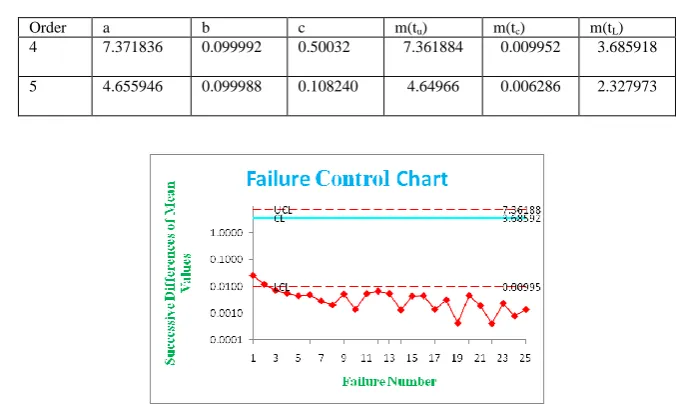
Table : 4 4Th and 5th order Parameter Estimates and control limits
Order a b c m(tu) m(tc) m(tL)
4 7.371836 0.099992 0.50032 7.361884 0.009952 3.685918
5 4.655946 0.099988 0.108240 4.64966 0.006286 2.327973
1275 |
P a g e
Figure 2 :Failure Control Chart of Table 3
IV. CONCLUSION
The 25 of 4th-order, 19 of 5th-order samples successive differences were plotted through the estimated mean
value function against the failure number. The parameter estimation is carried out by Newton Raphson Iterative
method for Burr model. The graphs have shown out of control signals i.e. below the LCL. Hence we conclude
that our method of estimation and the control chart are giving a +ve recommendation for their use in finding out
preferable control process or desirable out of control signal. By observing the Mean value Control chart we
identified that the failure situation is detected at 3rd to 25th points of table-2 for the corresponding m(t) in 4th
-order statistics and at 3rd to 19th point of table-3 for the corresponding m(t) in 5th-order statistics, which is below
m(tL). It indicates that the failure process is detected at an early stage. The early detection of software failure
will improve the software Reliability. When the time between failures is less than LCL, it is likely that there are
assignable causes leading to significant process deterioration and it should be investigated. On the other hand,
when the time between failures has exceeded the UCL, there are probably reasons that have lead to significant
improvement.
V. REFERENCES
[1]Musa J.D, Software Reliability Engineering MCGraw-Hill, 1998.
[2]N. Boffoli, G. Bruno, D. Cavivano, G. Mastelloni; Statistical process control for Software: a systematic
approach; 2008 ACM 978-1-595933-971-5/08/10. M. R. Lyu, Handbook of Software Reliability
Engineering, McGraw-Hill and IEEE Computer Society, pp. 27-164, New York, 1996.
[3]K. U. Sargut, O. Demirors; Utilization of statistical process control (SPC) in emergent software
organizations: Pitfallsand suggestions; Springer Science + Business media Inc. 2006. Jahir Pasha,
S.Ranjitha, Dr. H. N. Suresh,” Certain Reliability Growth Models for Debugging in Software Systems,
International Journal of Engineering and Technical Research (IJETR) Volume-2, Issue-4, April 2014
[4]Burr,A. and Owen ,M.1996. Statistical Methods for Software quality . Thomson publishing Company. ISBN
1-85032-171-X.Maria Teresa Baldassarre, Nicola Boffoli and Danilo Caivano, “Statistical Process Control
for Software: Fill the Gap” ,www.intechopen.com,2010
[5]Carleton, A.D. and Florac, A.W. 1999. Statistically controlling the Software process. The 99 SEI Software
Engineering Symposimn, Software Engineering Institute, Carnegie Mellon University
1276 |
P a g e
ACM 1-59593-085-x/06/0005.
[7]M. R. Lyu, Handbook of Software Reliability Engineering, McGraw-Hill and IEEE Computer Society, pp.
27-164, New York, 1996.
[8]Hong-Wei Liu, Xiao-Zong Yang, Feng Qu, and Yan-Jun Shu, “A General NHPP Software Reliability
Growth Model with Fault Removal Efficiency”, Iranian Journal of Electrical and Computer
Engineering,Vol. 4, No. 2 Summer-Fall 2005
[9]Goel. A.L and Okumoto. K., (1979). “A Time-dependent error-detection rate model for software and other
performance measures”, IEEE Trans. Reliability, vol R-28, Aug, pp 206 - 211.
[10] W. Burr, “Cumulative frequency functions,” Annals of Mathematical Statistics, vol. 13, pp. 215–232,
1942.
[11] Balakrishnan.N, Clifford Cohen; Order Statistics and Inference; Academic Press Inc; 1991.
[12] N.Boffoli,G.Bruno,D.Caivano,G.Mastelloni; “Statistical Process Control for Software: a Systematic
Approach”;2008 ACM 978-1-595933-971-5/08/10.
[13] Pham. H., “Handbook of Reliability Engineering”, Springer. 2003.
[14] Hoang Pham, “System Software Reliability”, Springer ,2006.
[15] M.Xie, T.N. Goh, P. Rajan; Some effective control chart procedures for reliability monitoring; Elsevier
science Ltd, Reliability Engineering and system safety 77(2002) 143- 150
[16] K.Ramchand H Rao, R.Satya Prasad, R.R.L.Kantham; Assessing Software Reliability Using SPC – An
Order Statistics Approach; IJCSEA Vol.1, No.4, August 2011.
[17] Michael R.Lyu 1996a, Handbook of Software Reliability Engineering.
[18] K.Sita Kumari, R.Satya Prasad;Pareto Type II Software Reliability Growth Model – An Order Statistics
Approach; IJCST Vol.2, Issue 4, Jul-Aug 2014.
[19] V.K.Gupta, Gaurav Aggarwal; Software Reliability Growth Model; IJARCSSE Vol.4, Issue 1, January
2014.
[20] Dr R.Satya Prasad, N.Geetha Rani, Prof R.R.L Kantham; Pareto Type II Based Software Reliability
Growth Model; IJSE Vol.2, Issue 4, 2011.
[21] Hee-cheul Kim., “Assessing Software Reliability based on NHPP using SPC”, International Journal of
Software Engineering and its Applications, vol.7,No.6 (2013), pp.61-70.
[22] R.Satya Prasad, K.V Murali Mohan, G.Sridevi;Burr Type XII Software Reliability Growth Model;IJCA
Volume 108 No-16 December 2014.
[23] Ch.Smitha Chowdary, Dr R.Satya Prasad, K.Sobhana;Burr Type III Software Reliability Growth
Model;IOSR-JCE Volume17,Issue 1,Jan-Feb 2015.
[24] Dr R.Satya Prasad,K.Ramchand H Rao, Dr R.R.L.Kantham ; “Software Reliability with SPC”