Reliability of Dynamic Multi-State Oil Supply System by Structure Function

(1)

Copyright to IJIRSET www.ijirset.com 13548

Reliability of Dynamic Multi-State Oil Supply

System by Structure Function

Fadhel S. F.1, Alauldin N. A.1 and Ahmed Y. Y.2

Department of Mathematics and Computer Applications, College of Science, Al-Nahrain University, Baghdad, Iraq1.

Information and Communication Technology Center, University of Technology, Baghdad, Iraq2.

ABSTRACT: Application of mathematical model of multi state system for oil supply system is considered in this paper. This paper describes a method for estimation of changes of one component states and its influence on themultistate system reliability by dynamic reliability indices. We examine the oil supply system to allow a different number of states for the oil supply system and for each pipelineby proposing dynamic reliability indices for investigation of this system. These indices estimate the influence upon the multi-state system reliability, which is the oil supply system from an oil source to three stations through several oil pipelines, say four. The mathematical approach of logical differential calculus is used for analysing the change in the multi-state system reliability that is caused by modification of some system components states.

KEYWORDS:Multistate system reliability, Structure function, Dynamic reliability indices, Direct partial logic derivatives.

I. INTRODUCTION

Hardware reliability has been increased by technological advances in large complex systems such as nuclear power plants, aircraft, and offshore oil plants, [16]. The basic concepts of MSS reliability were primarily introduced in the mid of the 1970's by Murchland in 1975, [11], [9], [3] and Ross in 1979, [14].Barlow and Wu in 1978 [1] characterize component state criticality as a measure of how a particular component state affects a specific system state.Griffithin 1980 [6] formalized the concept of MSS performance, and studied the impact of component improvement on the overall system reliability behaviour.The concepts of MSS important were also discussed in Block and Savits in1982 [2], where a decomposition theorem for MSS structure function was proved. Since that time, MSS reliability began with an intensive development. Essential achievements that were attained up to the mid of 1980's were reflected by Natvig in1985 [12], and by El-Neveihi and Prochan in 1984 [4], where it can be found the state of the art in the field of MSS reliability at this stage.

Readers that are more interested in the history and more ideas related to MSS reliability theory for the later work can find the corresponding overview in Lisnianski and Levitin [9] and Natvig [13].

There are some mathematical models in the reliability analysis. Firstly, it is the Binary System: the system and its components are allowed to have only two possible states (completed failure and perfect functioning). Secondly, it is the Multi-State System (MSS). In a MSS, both the system and its components may experience more than two states, for example, completely failed, partially functioning and perfect functioning. The reliability analysis of the binary system has served as a foundation for the mathematical treatment of the reliability theory. Many problem of the binary system have been settled. But this approach fails to describe many situations where the system can have more than two distinct states [9], [8]. Many practical components and systems have more than two different performance levels. For example, a power generator in a power station can work at full capacity, which is its nominal capacity, say 10MW, when there is no failure at all, [9]. Certain types of failures can cause the generator to be completely failed, while other failures will lead to the generator working at a reduced capacity say at 4 MW.

On the system level, let us consider a power generating system consisting of several power generators. The abilities of the system to meet high power load demand, normal power load demand and lower power load demand can be regarded as different system states.

(2)

spot B, i.e., spot A and B; it is in state 3 if the oil can reach up to spot C. In the paper [19] authors had substantiated basic conceptions to apply the direct partial logic derivatives (it is part of logical differential calculus) for the reliability analysis of MSS. The direct partial logic derivatives reflect changing the value of investigation function when the values of its variables change. In [17] the new class of reliability indices was determined and was named dynamic reliabilityindices(DRI). The dynamic character of DRI consists to determine states of the system failure or, in other case, to the repair system is caused by a change of state the system component. In other words, these indices define the boundary states of MSS. In paper [21] three groups of DRI were obtained the dynamic reliability indices which define the boundary states of MSS are given and the conditions of being and changing of these states depending on the change of the system component states have been considered. However, these indices have high dimensionality and there are problems in their application for real-word engineering problems include three groups of probabilistic indices, [23]: Dynamic deterministic reliability indices (DDRI’s), component dynamic reliability indices (CDRI’s) and dynamic integrated reliability indices (DIRI’s). The DDRI’s evaluate an influence of a level change of a component state on system reliability. Numerical DDRI is defined as sets of the system states. These sets are calculated by direct partial logic derivatives. The CDRI’s allows measuring an influence of each individual component to the system reliability. The DIRI’s represent how change of one of system components impacts to the system reliability. But these indices permits to analyses the influence of one component state change to MSS reliability only.

In this paper we evolve an application of MSS reliability analysis methods for representation and estimation of system with “oil supply system”.

II. PROBLEMFORMULATIONANDDESCRIPTIONOFSYSTEMMODEL

The MSS and each of -components can be in one of possible states: from the complete failure (it is 0) to the perfect functioning (it is −1) and has possible values. A structure function is one of typical representations of MSS and defines correlation of system performance level depending on MSS components states, [9]. Every system component

,∀ = 1,2, … , ; is characterized by probability of the performance rate:

, = { = }(1)

where = 1,2, … , and = 0,1, … , −1 .

The system reliability (system state) depends of its components state and is defined by the structure function:

Φ(x) =Φ( , , … , ): {0, … , −1} →{0, … , −1} (2)

The following assumptions are used for structure functions as shown in Equation (2) that are peculiar to reliability analysis, [7], [8]:

a) The structure function is non-decreasing and so: Φ( , , … , ) = ,Φ(0,0, … ,0) = 0 andΦ(x)≤ Φ(x )if x≤ x b) The behaviour of each component is mutually s-independent;

c) The every component is relevant to the system

The structure functions of parallel, series and k-out-of-n MSS terms are declared by OR (∨) and AND (∧), [18]:

Φ (x) =⋁ (3)

Φ∅ (x) =⋀ (4)

Φ(x) =⋁(⋀ ) (5)

where ⋁ = ( , , … , ) ;⋀ = ( , , … , ) The mathematical model of MSS k-out-of-n (5)can simplify by:

… ∨ … = …

and define as:

Φ(x) =⋁(⋀ ) (6)

For example, the structure functions MSS 2-out-of-3 is presented by:

Φ(x) = ⋁ ⋁ ⋁

The MSS 2-out-of-3 structure function is declare in this case:

( ) = ⋁ ⋁

A parallel system structure function is 1-out-of-n system:

Φ(x) =⋁(⋀ ) =⋁ (7)

And a series system structure function is n-out-of-n MSS:

(3)

III. DIRECTPARTIALLOGICDERIVATIVEFORMSSMODEL

The direct partial logic derivative of function Φ(x)with respect to the component ,∀ = 1,2, … , which is termed

Φ( → ℎ)/ ( → )reflects the fact of changing of the function Φ from state to state ℎ,when the value of component changing from a to b [22]:

( → ℎ)⁄ ( → )= ( , ) • ( , )(9)

where:

( , ) = ( , … , , … , , … , ); and ( , ) = ( , … , , … , , … , );

,ℎ ∈{0, 1, … , −1} and , ∈{0,1, … , −1}; and “•” is the symbol of a comparison operation, defined by:

( → ℎ)

( → )=

−1

0

, ( , ) = ( , ) =ℎ

, ℎ

So, the direct partial logic derivative of the structure function allows to examine the influence of the state change of the − ℎcomponent into the system reliability. In other words this derivative discovers the system states that are transformed as a result of the change of the component state, [23].

IV.MULTISTATESYSTEMFAILUREANDREPAIROFMSS,[23]

Direct partial logic derivative of the structure function allows to examine the influence of the − ℎ component state change into the system reliability. In other words this derivative discovers the system states that are transformed as a result of the change of the component state.

Consequences of the direct partial logic derivatives are of interest for reliability analysis of the MSS for this purpose, consider the following two partial derivatives:

∂Φ( →0)⁄∂ ( → )for j, ∈{1,2, … , −1} and ∈{0,1, … , −1}, <

Φ(0→ ℎ)⁄ ( → ) ℎ ∈{1,2, … , −1} and , ∈{0,1, … , −1}, <

The first derivative is a mathematical representation for the model of the system failure if the − ℎ component state changes from a to b. Because the structure function Φ( ) is non-decreasing, this derivative is Φ( →0)⁄ ( → −1); where , ∈{1,2, … , −1}.

The second derivative permits the mathematical description of the system renewal. There are two variants of investigation for the system repairing. First it is the system repairing by the replacement of the failure component. This situation is determined by the direct partial logic derivative Φ(0→ ℎ)/ (0→ −1). Second, it is the increase of component state that is described as Φ(0→ ℎ)/( ( → + 1) . However, the first variant is more important for applications. Because the structure function of the MSS is non-decreasing, this derivative can be assigned as

Φ(0→ ℎ)⁄ (0→ −1).

It is remarkable that direct partial logic derivatives allow to analyze dynamic properties of the MSS, which is submitted as structural function.

V. DYNAMICRELIABILITYINDICES

Dynamic reliability indices characterize the change of the MSS reliability that is caused by the change of a component state and include three groups of probabilistic indices: dynamic deterministic reliability indices(DDRI’s), component dynamic reliability indices (CDRI’s) and dynamic integrated reliability indices (DIRI’s). Therefore, we will explain next each of these concepts in details.

Definition (1) (Dynamic Deterministic Reliability Indices), [20], [21]:

Dynamic deterministic reliability indices are sets of the boundary state of the system { }(for system failure) and { }(for system repairing).

The states system failure { } and the states system repairing { }are defined by: = ∪ ∪…∪ (10)

{ } = { | }∪{ | }∪…∪{ | } (11)

where the subsets and { | }are defined by: = Φ( →0)⁄ ( →0)≠0 (12)

(4)

where { | } and{ | }are subsets of the boundary state of the system for everyone of system component ,∀ =

1,2, … , .

Definition (2) (Component Dynamic Reliability Indices), [21], [18]:

Component dynamic reliability indices are probabilities of MSS failure and repairing at a modification of a state of

− ℎ system component

= ( ) →_→ × ( ) (14)

= ( )→→ × ( ) (15)

where ( ) →_→ is the probability of the − ℎ component state modification from a to ( −1) where the system fail; ( )is the probability of state of − ℎ component; ( ) →→ is the probability of − ℎ component replace for

system repairing; ( )is the probability of − ℎ component failure.

( ) _→→ ₌ ( )→

→

× ×…× (16)

( ) →→ =

( ) _→→

× ×…× (17)

( ) →_→ is the number of system states when a change − ℎcomponent state from a to ( −1) forces the system failure; and ( ) →→ is number of system states when system repairing bring about by to replace − ℎ component.

Noting that, the numbers ( ) →_→ and ( ) _→→ _{are obtained as numbers of values of direct partial logic derivative}

(→ )

( → ) and

( → )

( → )with respect to the − ℎvariable, which are not equal 0.

In other words numbers ( ) →_→ and ( ) →→ are the cardinality of the set { | } in eq. (12) and the set { | } in

eq. (13) accordingly.

Definition (3) (Dynamic Integrated Reliability Indices), [19], [21]:

Dynamic integrated reliability indices is probability of the system failure or repairing if one of system component fails or restores, the failure and repair probability defined by:

=∑ ( ) ×∏ _, 1− ( ) (18)

=∑ ( ) ×∏ _, 1− ( ) (19)

where ( ) and ( ) is determined in equations (14) and (15).

VI.ILLUSTRATIVEEXAMPLES

In this section, we shall study general example of MSS model for investigation of its dynamic behavior. Example (1):

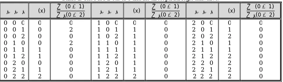
The direct partial logic derivative of the structure functionwith = 3, = 1,2,3, Φ(0→1)⁄ (0→2), which corresponds to description of MSS 2-out-of-3, are given in Table 1.

Table 1: The MSS 2-out-of-3 and the direct partial logic derivative.

, , Φ(x) Φ(0→1)

(0→2) , , Φ(x)

Φ(0→1)

(0→2) , , Φ(x)

Φ(0→1)

(0→2)

0 0 0 0 0 1 0 0 2 0 1 0 0 1 1 0 1 2 0 2 0 0 2 1 0 2 2

0 0 0 0 1 1 0 1 2 0 2 0 2 0 0 0 0 0

1 0 0 1 0 1 1 0 2 1 1 0 1 1 1 1 1 2 1 2 0 1 2 1 1 2 2

0 1 1 1 1 1 1 1 2 0 0 0 0 0 0 0 0 0

2 0 0 2 0 1 2 0 2 2 1 0 2 1 1 2 1 2 2 2 0 2 2 1 2 2 2

(5)

We will consider in this section the MSS of 2-out-of-3, where the structure function Φ(x)depends on three variables which are the system components = 3 and has the best level of the components = 3, ( = 1,2,3).

The used probabilities of the component state supported by expert which are given in Table (2).

Table 2: Component state probability.

Component State

0 1 2

0.1 0.6 0.3

0.4 0.5 0.1

0.2 0.2 0.6

We can calculate the CDRI for a 2-out-of-3 system which are presented in Table (3).

Table 3: CDRI calculation for parallel system (MSS 2-out-of-3).

( ) _→→ _{( )}

→

→ _{( )}

→

→ _{( )}

→

→ _{( )} _{( )}

4 2 0.148 0.074 0.089 0.022

4 2 0.148 0.074 0.074 0.007

4 2 0.148 0.074 0.029 0.044

Therefore the analysis of CDRI may be analyzed as follows:

a) The system has the maximum probability of failure when the firstcomponent is in failure state because its CDRI has the largest value (1) = 0.089.

b) The system fails with minimum probability if the third component has failed (3) = 0.029.

c) The MSS repairs with maximum probability by replacement of the third component since CDRI , (3) = 0.044. Finely, the DIRI permits to obtain the probability of the system failure if one of the system components is breakdown. It is = 0.17, while the probability of the system repairing is = 0.071if one of the failure components of the system is replaced.

VII. DYNAMICRELIABILITYOFOILSUPPLYSYSTEMMODEL

Many engineering systems can fit into the proposed multi state system model. In this section, we will present on applications that have been identified by Tian, Z., Li, W. and Zuo, M. J., [15], Similar applications can be found in power supply systems and telecommunication systems.

Consider for example an oil supply system, as shown in Figure (1).

(6)

The oil is delivered from the oil source to three stations through four oil pipelines. A pipeline is considered to be a multi-state component (thus n 4). A failure might occur at any part of a pipeline. Take pipeline 1 for example, if there is a failure in section , the section of pipeline 1 between the oil source and station 1, the oil will not be able to reach any station via pipeline 1. If there are no failures in section , but there is a failure in section , the section of pipeline 1 between station 1 and station 2, the oil will be able to reach station 1 but will not be able to reach station 2 or beyond. Similarly, if there is no failure in section or section , but there is a failure in section , the oil will be able to reach station 1 and station 2, but will not be able to reach station 3. Based on the possible failures in different sections of a pipeline, four states of a pipeline can be defined as follows:

1. State 0: oil cannot reach any stations. 2. State 1: oil can reach only station 1. 3. State 2: oil can reach station 1 and 2. 4. State 3: oil can reach station 1, 2 and 3. Each station has different demands on the oil.

1. Station 1: requires at least one pipelines working to meet its demand. 2. Station 2: requires at least two pipelines working to meet its demand. 3. Station 3: requires at least four pipelines working to meet its demand.

At the system level, we are interested in whether the demands of up to a certain station can be met. Thus, four states of the oil supply system can be defined as follows:

1. System state 0: it cannot meet the oil demand of station 1.

2. System state 1: it can meet the oil demand of up to station 1. That is, the system can meet the demand of station 1, but cannot meet the demand of station 2.

3. System state 2: it can meet the oil demands of up to station 2. That is, the system can meet the demands of station 1 and station 2, but cannot meet the demand of station 3.

4. System state 3: it can meet the oil demands of up to station 3. That is, the demands of station 1, 2 and 3 can all be met.

In practice, we may be interested in the probability of the oil supply system in states 0, 1, 2 or 3.

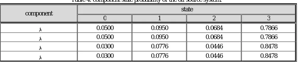
If , = 1,2,3,4 are used for the pipeline, then, the component state probability are given in table (4)

Table 4: component state probability of the oil source system.

component state

0 1 2 3

0.0500 0.0950 0.0684 0.7866 0.0500 0.0950 0.0684 0.7866 0.0300 0.0776 0.0446 0.8478 0.0300 0.0776 0.0446 0.8478

Note the structure function of MSS in this example hasdimension is = 4 = 256.

The structure function released to this system and the direct partial logic derivative Φ(1→0)⁄ (1→0) are found using computer programs and the subsets failure system { | }are therefore found to be:

a) { | }  {1000}, if the section is a failure, the oil will not be able to reach any station via pipeline 1. b) { | }  {0100}, if the section is a failure, the oil will not be able to reach any station via pipeline 2. c) { | } {0010}, if the section is a failure, the oil will not be able to reach any station via pipeline 3. d) { | } {0001}, if the section is a failure, the oil will not be able to reach any station via pipeline 4.

Also, the direct partial logic derivative Φ(1→2)⁄ (0→ ) are calculated using computer program for (i 1, 2, 3,4) and the analysis of this derivative permits to obtain states of the system failure for which the replacement of the broken component restores the system.

(7)

a) { | } ={0002,0003,0012,0013,0020,0021,0030,0031,0102,0103,0112,0113,0120,0121,0131,0200,0201,0210,021

1,0300,0301,0310,0311}, if there is no failure in sections , , and .

b) { | }={0002,0003,0012,0013,0020,0021,0030,0031,1002,1003,1012,1013,1020,1021,1030,1031,2000,2001,201 0,2011,3000,3001,3010,3011}, if there is no failure in sections , , and .

c) { | }={0002,0003,0102,0103,0200,0201,0300,0301,1002,1003,1102,1103,1200,1300,1301,2000,2001,2101}, if there is no failure in section , , and .

d) { | }={0020,0030,0120,0130,0200,0210,0300,0310,1120,1130,1200,1210,1300,1310,2000,2010,2100,2110,300 0,3010,3100,3110,}, if there is no failure in sections , , and .

VIII. SIMULATIONANDRESULTS

The results of the CDRI for the oil supply system are presented in Table (5).

Table 5: CDRI calculation for oil supply system.

( ) _→→ _{( )}

→

→ _{( )}

→

→ _{( )}

→

→ _{( )} _{( )}

1 23 0.003 0.089 0.00028 0.07000

1 24 0.003 0.093 0.00028 0.07315

1 18 0.003 0.07 0.00023 0.05934

1 22 0.003 0.085 0.00023 0.07206

So, the breakdown of the section and section causes the maximum probability of system failure ( (1) =

0.00028) and ( (2) = 0.00028). Section and have an influence on the system failure least of all ( (3) =

( (4) = 0.00023). The system repairing has its most value probable if there is no failures in sections , , and in

,( i. e. P (2) = 0.07315).

Also, The DIRI are probabilities of the change of the system reliability if the state of one of the system components is changed. The probability of the system failure, if one of the components breaks down, is = 0.001in accordance to eq. (18). The probability of system repairing obtained by eq. (19) and is = 0.2219if one of the failed components of the system is replaced.

IX.CONCLUSIONANDDISCUSSION

In this paper a new measure for MSS reliability is presented, which is calculated by using the structure function of MSS model for certain system network. This model allows to determine some level of system availability in contrast to the binary system. The MSS model is improved moreover: the system has a different number of discrete states for the system and for each component. This measure, which is labeled as DRI, involves the probabilities of the changes of the system states that are assigned by changes of component states. We consider two system changes: the system failure and system repair. But the suggesting method for reliability analysis of the MSS can be used to estimate the other changes in the system state. The dynamic reliability approach has been used successfully to evaluate the probability of the failure and repairing of the oil supply system as a real life application of dynamic multi-state k-out-of-n system model where the components and the system have multiple performance levels.All computational results are made by MATLAB program.

REFERENCES

[1] Barlow, W. and Wu, A., “Coherent Systems With Multi-State Components”, Math. Oper. Res., Vol. 3, pp. 275–281, 1978.

[2] Block, H. and Savits T., “A Decomposition of Multi State Monotone System”, J. Appl. Prob., Vol. 19, pp. 391–402, 1982.

[3] Boedigheimer, R. A., “Customer-Driven Reliability Models for Multistate Coherent Systems”, Ph.D. Thesis, University of Oklahoma, Norman,

1992.

[4] El-Neweihi, E. and Proschan, F., “Degradable Systems: a Survey of Multistate System Theory”, Commun Stat Theory Methods, Vol. 13, pp.

405–432, 1984.

[5] El-Neweihi, E., Proschan, F. and Sethuraman, J., “Multi-State Coherent Systems”, J. Appl. Prob., Vol. 15 , pp. 675-688, 1978.

[6] Griffith, W. , “Multi-State Reliability models” J. Appl. Prob., vol. 17, pp. 735-744, 1980.

[7] Huang, J. and Zuo, M.J., “Generalized Multi-State k-out-of-n:G System”, IEEE Transactions on Reliability, Vol. 49 (1), pp. 105–111, 2000.

[8] Huang, J. and Zuo, M.J., “Multi-State k-out-of-n System Model and its Applications”, ProcIntSymp. on Annual Reliability and Maintainability,

pp. 264-268, 2000.

(8)

[10]Min, X., Yuan, S. D. and Kim, L. P, “Computing System Reliability Models and Analysis”. New York, Boston, Dordrecht, London, Moscow,

2004.

[11]Murchland, J., “Fundamental Concepts and Relations for Reliability Analysis of Multi-State Systems and Fault Tree Analysis,” in Theoretical

and Applied Aspects of System Reliability, SIAM, pp. 581–618, 1975.

[12]Natvig, B., “Multi-State Coherent Systems”, in Encyclopedia of statistical sciences, Wiley, New York, Vol. 5.: pp. 732–735, 1985.

[13]Natvig, B., “Multi-State Reliability Theory”, In: Ruggeri F. Kenett, R. Faltinfw (eds) Encyclopediaof Statistics in Quality and Reliability, Wiley,

New York, pp. 1160–1164, 2007.

[14]Ross, S. M., “Multivalued State Component Systems”, Annals of Probability, Vol. 7(2), pp.379–383, 1979.

[15]Tian, Z., Li, W. and Zuo, M. J., “Multi-State k-out-of-n Systems and their Performance Evaluation”, IIE Transactions, Vol. 41, pp. 32–44, 2009.

[16]Zaitseva, A. and Puuronen, S., “Multi-State System in Human Reliability”, IEEE Transactions on Reliability, Vol. 978(1), pp. 4244-3960, 2008.

[17]Zaitseva, E. and Levashenko, V, “New Dynamic Relia- bility Indices for Multi-State System”, Proc 3rd IntConf on Mathematical Methods in

Reliability: Methodology and Practice, pp. 687-690, 2002.

[18]Zaitseva, E. and Levashenko, V., “Dynamic Reliability Indices for Parallel, Series and k-out-of-n Multi-State System”, in Proc. of the IEEE

52nd Annual Reliability & Maintainability Symposium (RAMS), pp.253 – 259, 2006.

[19]Zaitseva, E. and Levashenko, V., “Design of Dynamic Reliability Indices”, Proc IEEE 32th IntSymp on Multiple-Valued Logic, pp. 144-148,

2002.

[20]Zaitseva, E. and Levashenko, V., “New Reliability Indices for Multi-State System”, Proc 15th IEEE European Conf on Circuit Theory and

Design, 345–349, 2001.

[21]Zaitseva, E., “Dynamic Reliability Indices for Multi-State System”, Journal of Dynamic System & Geometric Theories, Vol. 1 No. 2, pp.

213-222, 2003.

[22]Zaitseva, E., “Reliability Analysis of Multi-State System, Dynamical Systems and Geometric Theories”, Vol. 1 (2), pp.213-222, 2003.

[23]Zaitseva, E., Levashenko, V. and Matiasko, K., “Reliability Analysis of Dynamic Behavior for Multi-State System”, Proc. Stochastic Models in

Reliability, Safety, Security and Logistics Symp., (February), pp.386-389, 2005.

BIOGRAPHY

Asst. Prof. Dr.Fadhel S. F. is the head of Mathematics and Computer Applications Department, College of Science, Al-Nahrain University, Baghdad-Iraq. He is received the Ph.D. in 1998, were he is the supervisor of more than 40 M.Sc. Student and 7 Ph.D. Students, in which the fields of interest are those topics related to fuzzy set theory, stochastic differential equations and numerical analysis.

Prof. Dr.Alauldin N. A. has complete his Doctorate of Philosophy in 1986. He is currently working as Professor at the Department of Mathematics and Computer Applications, College of Science, Al-Nahrain University, Baghdad-Iraq and guiding M.Sc. and Ph.D. students.