Seismic Analysis and Design of Type FR Steel Frames Using Displacement-Based Design and Advanced Analysis

(1)

Abstract

HARRIS III, JOHN LEROY. Seismic Analysis and Design of Type FR Steel Frames Using Displacement-Based Design and Advanced Analysis. (Under the direction of Mervyn J. Kowalsky.)

Current design office methodologies for seismic design of steel moment frames include forced-based methods for calculating equivalent lateral forces and a static elastic analysis. Research has revealed erroneous assumptions in forced-based methods and proposes that displacement-based methods, due to modeling inelastic systems, result in more reasonable lateral force distributions. Additionally, LRFD1 member design interaction equations implicitly account for geometric and material non-linear effects. This philosophy does not satisfy compatibility between actual inelastic member response and the elastic system as assumed by a conventional elastic analysis.

(2)

The goal of this research is to advance the validity and accuracy of displacement-based design methods and Advanced Analysis for the engineering of seismic resistant steel moment frames. This research will allow the development of alternate seismic analysis and design procedures, as well as refined practical methods that can be incorporated in a design office.

(3)

SEISMIC ANALYSIS AND DESIGN OF TYPE FR STEEL

FRAMES USING DISPLACEMENT-BASED DESIGN AND

ADVANCED ANALYSIS

by

JOHN LEROY HARRIS III

A thesis submitted to the Graduate Faculty of North Carolina State University

in partial fulfillment of the requirements for the Degree of

Master of Science

CIVIL AND ENVIRONMENTAL ENGINEERING

Raleigh

2002

APPROVED BY:

_________________________________

Tasnim Hassan

_________________________________

James Nau

________________________________

Chair of Advisory Committee

(4)

Unquestioned answers are more dangerous than unanswered questions

Unknown

Dedicated to

(5)

Biography

John Harris was born August 8, 1970 in Rome, NY and spent his childhood years in Chicago, IL, and Raleigh, NC. After completing his Bachelor of Science degree in Civil Engineering at North Carolina State University in 1994, he worked as a Structural Engineer in Raleigh, NC, Atlanta, GA, and New York, NY, with special interest in steel structures. Additionally, John is a registered Professional Engineer and an active member of AISC, SSRC, and ASCE. For the past several years, he has participated with various industry committees, most

notably, Committee on Manuals and Textbooks for AISC and Task Group #29 – 2nd Order

Inelastic Analysis for SSRC. It was the experience with these groups that led John to return to North Carolina State University with an interest in researching Advanced Analysis techniques for steel structures. While at NCSU, John met Mervyn Kowalsky, who strengthened John’s concentration in earthquake engineering, and began researching displacement-based seismic design and Advanced Analysis of steel frames. John completed his Master of Science degree in August 2002.

(6)

Acknowledgements

I am sincerely grateful to the following while preparing this document.

• God, for giving me the ability to think, though at times incorrectly.

• My family and friends, whom without their support I would be a starving musician.

• Brian Lanier, Kirk Stanford, Randall Wilson, Joel Howard, Todd Garrison, Scott

Wirgau, and Tyler Durden, for putting up with my raving discussions, most notably, the ones concerning my ironic views that people should not live in severe earthquake prone regions. For the scientific exploration, I do submit.

• My mentor and friend, JC Smith, for the ability to see the truths in his vision.

• My committee members, Jim Nau and Tasnim Hassan, for their support, wisdom,

guidance, and their ability to let go at 4:30 on Friday.

• My committee chair, Mervyn Kowalsky, for showing me the light and then

(7)

List of Tables

Table 1.1-1 Frame description 4

Table 2.1-1 Structural performance levels 13

Table 2.1-2 Design level earthquakes 14

Table 2.1-3 Basic safety performance objective 15

Table 2.2.3-1 Recommended design magnitude of compressive

residual stresses 21

Table 2.2.5-1 Recommended material overstrength factors 28

Table 2.2.6-1 Recommended equivalent plastic curvatures 29

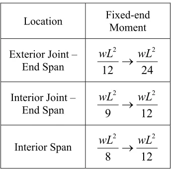
Table 2.3.3-1 Elastic fixed-end moments 38

Table 2.3.5-1 Recommended equivalent plastic rotation capacities 42

Table 2.3.5-2 Recommended equivalent plastic rotation capacities

with axial force 42

Table 2.4-1 Recommended target interstory drifts corresponding to rotation

demands 44

Table 2.4-2 Inelastic Displacement Profiles 44

Table 2.5-1 Frame descriptions 73

Table 2.5-2 Target interstory drifts per performance level 74

Table 2.5-3 Target peak ground accelerations per performance level 75

Table 2.5.1-1 Floor equivalent plastic rotations (FR-4) 81

Table 2.5.1-2 SP-1 target displacements (FR-4) 83

Table 2.5.1-6 SP-1 SDOF system properties (FR-4) 85

(13)

Table 2.5.1-10 SP-4 effective system properties (FR-4) 88

Table 2.5.1-14 Equivalent static lateral forces (FR-4) 90

Table 2.5.4-1 Floor equivalent plastic rotations (FR-4a) 101

Table 2.5.4-2 SP-1 target displacements (FR-4a) 103

Table 2.5.4-6 SP-1 SDOF system properties (FR-4a) 104

Table 2.5.4-10 SP-4 effective system properties (FR-4a) 106

Table 2.5.4-14 Equivalent static lateral forces (FR-4a) 107

Table 2.5.5-1 Floor equivalent plastic rotations (FR-4b) 110

Table 2.5.5-2 SP-1 target displacements (FR-4b) 110

Table 2.5.5-6 SP-1 SDOF system properties (FR-4b) 112

(14)

Table 2.5.5-10 SP-4 effective system properties (FR-4b) 113

Table 2.5.5-14 Equivalent static lateral forces (FR-4b) 114

Table 2.5.6-2 Elastic SP-1 target displacements (FR-8) 118

Table 2.5.6-6 Elastic SP-1 SDOF system properties (FR-8) 120

Table 2.5.6-13 Elastic SP-1 effective system properties (FR-8) 123

Table 2.5.7-1 Floor equivalent plastic rotations (FR-8-W27) 127

Table 2.5.7-2 Elastic SP-1 target displacements (FR-8-W27) 127

Table 2.5.7-3 SP-2 target displacements (FR-8-W27) 128

(15)

Table 2.5.7-7 SP-2 SDOF system properties (FR-8-W27) 130

Table 2.5.7-10 SP-4 effective system properties (FR-8-W27) 131

Table 2.5.7-13 Elastic SP-1 effective system properties (FR-8-W27) 132

Table 2.5.7-14 Equivalent static lateral forces (FR-8-W27) 132

Table 2.5.8-2 Elastic SP-1 target displacements (FR-16) 138

Table 2.5.8-6 Elastic SP-1 SDOF system properties (FR-16) 143

Table 2.5.8-13 Elastic SP-1 effective system properties (FR-16) 147

Table 4-1 Selected time-histories 175

Table 4.1.1-1 FR-4 Displacements at effective height 178

Table 4.1.2-1 FR-4 Maximum base shears 189

Table 4.2.1-1 FR-4-W21 Displacement at effective height 196

(16)

Table 4.3.2-1 Base shears (FR-4-W24) 205

Table 4.4.1-1 FR-4a Displacement at effective height 208

Table 4.4.2-1 FR-4a Base shears 211

Table 4.5.1-1 FR-4b Displacement at effective height 215

Table 4.5.2-1 FR-4b Base shears 218

Table 4.6.1-1 FR-8 Displacement at effective height 222

Table 4.6.2-1 FR-8 Base shears 231

Table 4.7.2-1 FR-8-W27 Base shears 239

Table 4.8.1-1 FR-16 Displacement at effective height 243

Table 4.8.2-1 FR-16 Base shears 252

(17)

List of Figures

Figure 1.1-1 Building plan 5

Figure 1.2.1-1 Member Force-Displacement graph of structural steel beam 7

Figure 1.2.1-2 Cyclic behavior of structural steel with Baushinger Effect 8

Figure 2.1-1 System Force-displacement graph 12

Figure 2.1-2 Graphical representation of structural performance levels 13

Figure 2.1-3 Structural Performance Objectives 14

Figure 2.2.2-1 Normalized moment-curvature graph 19

Figure 2.2.2-2 Elasto-perfectly plastic moment-curvature graph 19

Figure 2.2.3-1 Plastic flexural behavior of wide-flange with residual stresses 21

Figure 2.2.4.1-1 Idealized interaction diagram for steel beam-column 25

Figure 2.3.1-1 Beam-column subjected to end moments and axial force 30

Figure 2.3.2-1 Beam-Column subjected to end moments, axial force, and

support displacement 33

Figure 2.3.3-1 Beam-Column subjected to end moments, axial force, and

transverse load 34

Figure 2.3.3-2 Moment comparison 38

Figure 2.4-1 SDOF representation of actual system 43

Figure 2.4-1 Recommended Inelastic Displacement Profiles 45

Figure 2.4.3-1 Effective damping vs. ductility graph 50

Figure 2.4.4-1 Displacement Response Spectra 50

Figure 2.4.4-2 System force-displacement graph 52

Figure 2.4.5-1 Displacement profile ranges of frames 54

Figure 2.4.5.1-1 Non-linear yield displacement profile at SP-1 performance level 56

Figure 2.4.5.1-2 Normalized target drift to EQ level comparison 57

Figure 2.4.6.2-1 System Force-Deformation Graph including System Overstrength 64

(18)

Figure 2.4.6.3-1 Reduced cross-section at plastic hinge length 68

Figure 2.5-1 EQ I Displacement Response Spectrum

(PGA Reduction Factor = 0.125) 76

Figure 2.5-2 EQ II Displacement Response Spectrum

Figure 2.5-3 EQ III Displacement Response Spectrum

Figure 2.5-4 EQ IV Displacement Response Spectrum

Figure 2.5-5 Equivalent damping vs. displacement ductility 78

Figure 2.5.1-1 Frame schematic (FR-4) 79

Figure 2.5.1-2 Target displacement profiles (FR-4) 84

Figure 2.5.1-3 Equal displacement approximation 87

Figure 2.5.1-3 System force-displacement graph (FR-4) 89

Figure 2.5.1-5 Final frame schematic (FR-4) 93

Figure 2.5.1-6 SP-1 displacement profile (FR-4) 93

Figure 2.5.2-1 System force-displacement graph (FR-4-W21) 95

Figure 2.5.2-2 Final Schematic (FR-4-W21) 96

Figure 2.5.2-3 SP-1 displacement profile (FR-4-W21) 96

Figure 2.5.3-2 Final schematic (FR-4-W24) 98

Figure 2.5.3-3 SP-1 displacement profile (FR-4-W24) 99

Figure 2.5.4-1 Frame schematic (FR-4a) 100

Figure 2.5.4-2 Beam Rotation Chart 101

Figure 2.5.4-3 Beam rotation ductility chart 102

Figure 2.5.4-4 Target displacement profiles (FR-4a) 104

(19)

Figure 2.5.4-6 Final frame schematic (FR-4a) 108

Figure 2.5.4-7 SP-1 displacement profile (FR-4a) 108

Figure 2.5.5-1 Frame schematic (FR-4b) 109

Figure 2.5.5-2 Target displacement profiles (FR-4b) 111

Figure 2.5.5-3 System force-displacement graph (FR-4b) 114

Figure 2.5.5-4 Final frame schematic (FR-4b) 115

Figure 2.5.5-5 SP-1 displacement profile (FR-4b) 115

Figure 2.5.6-3 Elastic and pseudo-elastic non-linear displacement profiles 122

Figure 2.5.6-6 Elastic SP-1 Displacement Profile (FR-8) 126

Figure 2.5.7-1 Target displacement profiles (FR-8-W27) 129

Figure 2.5.7-3 Final Frame schematic (FR-8-W27) 134

Figure 2.5.7-4 Elastic SP-1 Displacement Profile (FR-8-W27) 135

Figure 2.5.8-5 Elastic SP-1 Displacement Profile (FR-16) 151

Figure 3.2.1-1 Two-surface stiffness degrading plastic hinge interaction diagram 158

Figure 3.2.1-2 Parabolic plastic hinge stiffness degradation function 159

Figure 3.2.1-3 CRC tangent stiffness degradation function 160

Figure 3.2.1-4 Normalized axial force-strain relationship 160

(20)

Figure 3.2.2-2 Comparison of strength curves 162

Figure 3.3.1-1 FR-4 System Force-Displacement Graph 165

Figure 3.3.1-2 FR-4 SP-1 Displacement Profile 165

Figure 3.3.2-1 FR-4-W21 System Force-Displacement Graph 166

Figure 3.3.2-2 FR-4-W21 SP-1 Displacement Profile 166

Figure 3.3.3-2 FR-4-W24 SP-1 Displacement Profile 167

Figure 3.3.4-1 FR-4a System Force-Displacement Graph 168

Figure 3.3.5-1 FR-4b System Force-Displacement Graph 169

Figure 3.3.5-2 FR-4b SP-1 Displacement profile 169

Figure 3.3.6-1 FR-8 System Force-Displacement Graph 170

Figure 3.3.6-2 FR-8 SP-1 Displacement Profile 170

Figure 3.3.7-2 FR-8-W27 SP-1 Displacement profile 171

Figure 4.1.1-1 FR-4 Maximum displacement envelopes (SP-1:EQ I) 176

Figure 4.1.1-2 FR-4 Maximum displacement envelopes (SP-2:EQ II) 177

Figure 4.1.1-3 FR-4 Maximum displacement envelopes (SP-3:EQ III) 177

Figure 4.1.1-4 Maximum displacement envelopes (SP-4:EQ IV) 178

Figure 4.1.1-5 FR-4 Nodal displacements as function of time (TH-1:EQ I) 180

Figure 4.1.1-6 FR-4 Interstory drifts as function of time (TH-1:EQ I) 181

Figure 4.1.1-7 FR-4 Nodal displacements as function of time (TH-1:EQ II) 182

Figure 4.1.1-8 FR-4 Interstory drifts as function of time (TH-1:EQ II) 182

Figure 4.1.1-9 FR-4 Nodal displacements as function of time (TH-1:EQ III) 183

Figure 4.1.1-10 FR-4 Interstory drifts as function of time (TH-1:EQ III) 184

Figure 4.1.1-11 FR-4 Nodal displacements as function of time (TH-1:EQ IV) 184

Figure 4.1.1-12 FR-4 Interstory drifts as function of time (TH-1:EQ IV) 185

(21)

Figure 4.1.1-14 FR-4 Maximum interstory drift envelopes (SP-1:EQ I) 187

Figure 4.1.1-15 FR-4 Maximum interstory drift envelopes (SP-2:EQ II) 187

Figure 4.1.1-16 FR-4 Maximum interstory drift envelopes (SP-3:EQ III) 188

Figure 4.1.1-17 FR-4 Maximum interstory drift envelopes (SP-4:EQ IV) 188

Figure 4.1.2-1 FR-4 System force-displacement graph 190

Figure 4.1.2-2 FR-4 Maximum story shear envelopes (SP-1:EQ I) 191

Figure 4.1.2-3 FR-4 Maximum story shear envelopes (SP-2:EQ II) 191

Figure 4.1.2-4 FR-4 Maximum story shear envelopes (SP-3:EQ III) 192

Figure 4.1.2-6 FR-4 story shears as function of time (TH-1:EQ III) 193

Figure 4.2.1-1 FR-4-W21 Maximum displacement envelopes (SP-1:EQ I) 194

Figure 4.2.1-2 FR-4-W21 Maximum displacement envelopes (SP-2:EQ II) 195

Figure 4.2.1-3 FR-4-W21 Maximum displacement envelopes (SP-3:EQ III) 195

Figure 4.2.1-4 FR-4-W21 Maximum displacement envelopes (SP-4:EQ IV) 196

Figure 4.2.1-5 FR-4-W21 Maximum interstory drift envelope (SP-1:EQ I) 197

Figure 4.2.1-6 FR-4-W21 Maximum interstory drift envelope (SP-2:EQ II) 197

Figure 4.2.1-7 FR-4-W21 Maximum interstory drift envelope (SP-3:EQ III) 198

Figure 4.2.1-8 FR-4-W21 Maximum interstory drift envelope (SP-4:EQ IV) 198

Figure 4.2.2-1 FR-4-W21 System force-displacement graph 199

(22)

Figure 4.4.1-1 FR-4a Maximum displacement envelopes (SP-1:EQ I) 206

Figure 4.4.1-2 FR-4a Maximum displacement envelopes (SP-2:EQ II) 207

Figure 4.4.1-3 Fr-4a Maximum displacement envelopes (SP-3:EQ III) 207

Figure 4.4.1-4 FR-4a Maximum displacement envelopes (SP-4:EQ IV) 208

Figure 4.4.1-5 FR-4a Maximum interstory drift envelope (SP-1:EQ I) 209

Figure 4.4.1-6 FR-4a Maximum interstory drift envelope (SP-2:EQ II) 209

Figure 4.4.1-7 FR-4a Maximum interstory drift envelope (SP-3:EQ III) 210

Figure 4.4.1-8 FR-4a Maximum interstory drift envelope (SP-4:EQ IV) 210

Figure 4.4.2-1 FR-4a System force-displacement graph 211

Figure 4.5.2-2 FR-4a Maximum story shears (TH-1) 212

Figure 4.5.2-3 FR-4a Maximum story shears (TH-2) 212

Figure 4.5.1-1 FR-4b Maximum displacement envelopes (SP-1:EQ I) 213

Figure 4.5.1-2 FR-4b Maximum displacement envelopes (SP-2:EQ II) 214

Figure 4.5.1-3 Fr-4b Maximum displacement envelopes (SP-3:EQ III) 214

Figure 4.5.1-4 FR-4b Maximum displacement envelopes (SP-4:EQ IV) 215

Figure 4.5.1-5 FR-4b Maximum interstory drift envelope (SP-1:EQ I) 216

Figure 4.5.1-6 FR-4b Maximum interstory drift envelope (SP-2:EQ II) 216

Figure 4.5.1-7 FR-4b Maximum interstory drift envelope (SP-3:EQ III) 217

Figure 4.5.1-8 FR-4b Maximum interstory drift envelope (SP-4:EQ IV) 217

Figure 4.5.2-1 FR-4b System force-displacement graph 218

Figure 4.5.2-2 FR-4b Maximum story shears (TH-1) 219

Figure 4.5.2-3 FR-4b Maximum story shears (TH-2) 219

(23)

Figure 4.6.1-14 FR-8 Maximum interstory drift envelope (SP-1:EQ I) 229

Figure 4.6.1-15 FR-8 Maximum interstory drift envelope (SP-2:EQ II) 229

Figure 4.6.1-16 FR-8 Maximum interstory drift envelope (SP-3:EQ III) 230

Figure 4.6.1-17 FR-8 Maximum interstory drift envelope (SP-4:EQ IV) 230

Figure 4.6.2-5 FR-8 Maximum story shear envelopes (SP-4:EQ IV) 233

Figure 4.7.1-8 FR-8-W27 Maximum interstory drift envelope (SP-4:EQ IV) 238

(24)

Figure 4.7.2-2 FR-8-W27 Maximum story shears (TH-2) 240

Figure 4.8.1-4 FR-16 Maximum displacement envelopes (SP-4:EQ IV) 243

Figure 4.8.1-14 FR-16 Maximum interstory drift envelope (SP-1:EQ I) 250

Figure 4.8.1-15 FR-16 Maximum interstory drift envelope (SP-2:EQ II) 250

Figure 4.8.1-16 FR-16 Maximum interstory drift envelope (SP-3:EQ III) 251

Figure 4.8.1-17 FR-16 Maximum interstory drift envelope (SP-4:EQ IV) 251

Figure 4.8.2-5 FR-16 Maximum story shear envelopes (SP-4:EQ IV) 254

Figure 4.9-1 MCE (EQ IV) Design displacement response spectrums

(5% damping) 255

(10% damping) 256

(25)

(20% damping) 257

(25% damping) 257

Figure 4.9-6 Displacement variations at effective system height (FR-4) 258

Figure 4.9-9 Range of effective system periods (FR-4) 260

Figure A.1-1 EQ I Acceleration Response Spectrum 271

Figure A.1-2 EQ II Acceleration Response Spectrum 271

Figure A.1-3 EQ III Acceleration Response Spectrum 272

Figure A.1-4 EQ IV Acceleration Response Spectrum 272

Figure A.2-1 EQ I Displacement Response Spectra 273

Figure A.2-2 EQ II Displacement Response Spectra 273

Figure A.2-3 EQ III Displacement Response Spectra 274

Figure A.2-4 EQ IV Displacement Response Spectra 274

Figure A.3-1 EQ I Velocity Response Spectra 275

Figure A.3-2 EQ II Velocity Response Spectra 275

Figure A.3-3 EQ III Velocity Response Spectra 276

Figure A.3-4 EQ IV Velocity Response Spectra 276

Figure B.1-1 Time-History (TH-1) 277

Figure B.1-2 Acceleration Response Spectra (TH-1) 277

Figure B.1-3 Displacement Response Spectra (TH-1) 278

Figure B.1-4 Velocity Response Spectra (TH-1) 278

(26)

(27)

(28)

List of Symbols

f

b Flange width

c Distance from extreme compression fiber to neutral axis

d Section depth

g Acceleration of gravity

sys eff

h System effective height

i

h Floor height

n

h Total frame height

w

h Height of web (inside of flange to inside of flange) (also d_w)

n Number of stories

r Radius of gyration

f

t Flange thickness

w

t Web thickness

w Uniform load

o

y Distance from extreme compression to centroidal axis

g

A Gross cross-sectional area

E Nominal Modulus of Elasticity

L

F Nominal yield stress including residual stresses

r

F Nominal compressive residual stress

x

F Lateral force

y

F Nominal material yield stress

ye

F Material yield stress including material overstrength (AISC)

(29)

G Stiffness ratio of interconnecting columns to beams

x

I Moment of inertia about major axis

K Slenderness factor

sys eff

K System effective stiffness

sys el

K System elastic stiffness

L Member length

Lb Beam length

Lc Column length

M Applied moment

B A

M _, Moment at end A or B

sys eff

M System effective mass

EQ

M Moment due to earthquake

G

M Moment due to transverse load(s)

i

M Floor mass

n

M Nominal section flexural resistance

o

M Total section plastic moment capacity

p

M Section plastic moment capacity

pc

M Reduced section plastic moment capacity for presence of axial force

ps

M Reduced section plastic moment capacity for presence of shear force

pt

M Reduced section plastic moment capacity for presence of torsion

pr

M Reduced section plastic moment capacity

r

M Section plastic moment capacity

T

(30)

y

M Section yield moment capacity

P Applied axial force (compression or tension)

n

P Nominal section axial resistance

u

P Ultimate axial force (compression or tension)

y

P Axial plastic nominal material yield stress

R Force reduction factor

y

R Material overstrength factor (AISC)

1

S One (1) second period spectral acceleration

F

S Shape factor

ii

s Beam-column stiffness coefficient

S

S Short period spectral acceleration

x

S Elastic section modulus about major axis

T Period

sys eff

T System effective period

p

T Section plastic torsion capacity

pt

T Reduced section plastic torsion capacity for presence of torsion

V Shear force

b

V Base shear

n

V Nominal section shear resistance

p

V Plastic shear capacity

u

V Ultimate shear force

i

W Floor weight

x

(31)

s

α Plastic moment capacity reduction factor for shear

β Ratio of SP-4 lateral force to performance level lateral force

∆ Displacement

i d

∆ Design, or target, nodal displacement

sys d

∆ System design, or target, displacement

sys p

∆ Post-yield system displacement

y

∆ Yield displacement

sys y

∆ System yield displacement

y

ε Nominal material yield strain

'

y

ε Nominal material first-yield strain

λ Column-to-beam stiffness factor

o

λ Total member overstrength

B A,

θ Member rotation at end A or B

d

θ Design joint rotation

G

θ Member rotation due to transverse load(s)

p

θ Equivalent member plastic rotation capacity

T

θ Target joint rotation

y

θ Member yield rotation capacity

φ Curvature

y

φ Section yield curvature

p

φ Equivalent section plastic curvature

'

y

(32)

x

φ Resistance factor

o m

φ Material overstrength

o ph

φ Member overstrength from plastic hinge sequencing

o i ph

φ Floor member overstrength from plastic hinge sequencing

o sys ph

φ System member overstrength from plastic hinge sequencing

o s

φ Member overstrength

o sys s

φ System member overstrength

o sf

φ Overstrength from shape factor

o sh

φ Overstrength from strain hardening

o i s

φ Floor member overstrength

o sr

φ Overstrength from strain rate

σ Stress

c

σ Compressive Stress

t

σ Tensile Stress

i

Ω Floor performance overstrength

sys

Ω System performance overstrength

µ Ductility

∆

µ Displacement ductility

sys

∆

µ System displacement ductility

θ

µ Rotation ductility

ς Damping

sys eff

(33)

List of Abbreviations

AISC American Institute of Steel Construction

ARS Acceleration Response Spectra

CRC Column Research Council

DBD Displacement-based Design

DFRD Demand and Resistance Factor Design

DRS Displacement Response Spectra

EPP Elasto-perfectly Plastic

EQ Earthquake

EYA Equivalent Yield Analysis

FBD Force-based Design

FEMA Federal Emergency Management Agency

IBC International Building Code

LRFD Load and Resistance Factor Design

MCE Maximum Considered Earthquake

MDOF Multi-degree-of-freedom

NEHRP National Earthquake Hazards Reduction Program

PBSE Performance-based Seismic Engineering

PGA Peak Ground Acceleration

SDOF Single-degree-of-freedom

SEAOC Structural Engineers Association of California

SP Structural Performance Level

(34)

1

PART 1

I

N

T

R

O

D

U

C

T

I

O

N

,

S

(35)

2

1.0 Introduction

The objective of this research is to outline an alternate seismic engineering philosophy to the current codified force-based design (FBD) approach for seismic resistant steel moment frames known as Performance-based Seismic Engineering (PBSE). Performance-based engineering is any design methodology in which the final analytical outcome is measured against a performance limit state. These limit states can be quantitatively measured by forces, strains, rotations, or displacements, and are representative of member or system damage levels. It is the limit state form that delineates the design methodology into respective performance-based groups. Since displacements are the most convenient practice of system and member evaluation, the analytical method employed in this research to achieve PBSE is Displacement-based Design (DBD).

(36)

3

Furthermore, current seismic codes limit inelastic story drifts to 0.02 or 0.025 depending on the initially “assumed” 1st mode period. These values are based on early research reporting that steel beams can accommodate post-yield rotations in the range of 0.01 to 0.015 radians – assuming an elastic rotation capacity of 0.01 radians (AISC Seismic Provisions, 2000). These rotation values have been subsequently revised based on later research; however, the codified inelastic drift requirements have not been similarly revised. As a consequence, code drift limits tend to reduce design ductility levels to values significantly less than what can actually be accommodated (Priestley and Kowalsky, 2000). Ultimately, the system will not be able to accommodate the full ductility demand (assumed equal to the force reduction factor by current seismic codes). Thus producing higher than expected seismic forces and possibly leading to either unexpected damage or damage levels in excess of desired. Furthermore, FBD procedures were developed based on the results from early scale model research and current research is noting that those results are not appropriate for determining or predicting the behavior of larger complex systems.

(37)

4

1.1 Current

Research

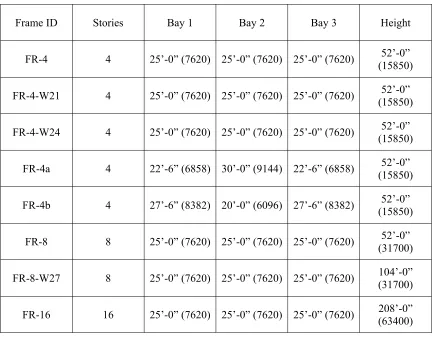
In this document, eight (8) fixed base steel moment frames, listed in Table 1.1-1, will be analyzed and designed in accordance with the proposed DBD method (Part 2).

Frame ID Stories Bay 1 Bay 2 Bay 3 Height

FR-4 4 25’-0” (7620) 25’-0” (7620) 25’-0” (7620) 52’-0”

(15850)

FR-4-W21 4 25’-0” (7620) 25’-0” (7620) 25’-0” (7620) 52’-0”

(15850)

FR-4-W24 4 25’-0” (7620) 25’-0” (7620) 25’-0” (7620) 52’-0”

(15850)

FR-4a 4 22’-6” (6858) 30’-0” (9144) 22’-6” (6858) _(15850)52’-0”

FR-4b 4 27’-6” (8382) 20’-0” (6096) 27’-6” (8382) 52’-0”

(15850)

FR-8 8 25’-0” (7620) 25’-0” (7620) 25’-0” (7620) 52’-0”

(31700)

FR-8-W27 8 25’-0” (7620) 25’-0” (7620) 25’-0” (7620) 104’-0” _(31700)

FR-16 16 25’-0” (7620) 25’-0” (7620) 25’-0” (7620) 208’-0” _(63400)

Table 1.1-1. Frame description

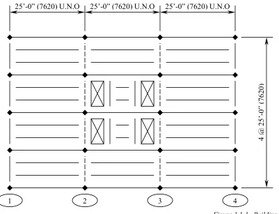
The selected test frame is the center frame (left to right) in the building plan shown in Fig. 1.1-1 (neglecting the floor openings).

(38)

5

Analysis, for the design of multi-story frames where the “yield” displacement profile is non-linear.

Figure 1.1-1. Building plan

Additionally, a limit state second-order inelastic static analysis, or “Advanced Analysis” will be used to analyze the frames designed by the proposed method (Part 3). The distinct difference between Advanced Analysis and a standard elastic analysis, including a push-over analysis, besides the obvious inclusion of inelastic response, is that all design uncertainties and imperfections inherent in current steel design interaction equations are included in the analysis. Thus eliminating the incompatibility between elastic analysis demands and inelastic capacities. The analysis results will be compared to the predicted values not necessarily as an acceptance analysis of the proposed method but to outline the initial use of Advanced Analysis techniques for the design of seismic resistant steel frames.

Finally, the frames will be analyzed in a second-order inelastic dynamic analysis subject to twelve (12) time-histories representing a wide analytical range of ground motions (Part 4). Two of the time-histories are artificially generated to approximate the MCE design

4

@

2

5’-0

”

(76

20

)

25’-0” (7620) U.N.O

25’-0” (7620) U.N.O 25’-0” (7620) U.N.O

(39)

6

acceleration response spectra developed in accordance with current IBC/NEHRP seismic provisions. Whereas the other actual time-histories are intensity normalized to the MCE design acceleration response spectra. The predicted, or “as designed”, response from the proposed method will be compared to the analysis results for applicability and to highlight future research needs.

This research represents the fundamental procedures outlining the preliminary development of Displacement-Based Design of steel moment frames. The analysis and design, including behavior, of steel structures increases in complexity as the number of joints increase. Behavior of steel frames is separated from analysis and design, though correlation exists, to emphasize the fact that in DBD the final behavior of the system justifies the analysis and design, not vice versa as in current force-based design procedures. Hence, several simplifications and assumptions have been used, outlined in Section 1.2, more for assistance in the basic understanding of steel response than for accuracy in the early development of the proposed procedures. It is the hope of the author to continue this research forward, continually revising the process for accuracy and simplicity, in order to develop a systematic design procedure.

(40)

7

1.2 Simplifications, Assumptions, and Constant Variables

The following items are used throughout this document, unless specifically noted otherwise.

1.2.1 Simplifications

1. Member Behavior

The bi-linear elasto-perfectly plastic approximation of the actual force-displacement response, shown in Fig. 1.1.1-1, is used as the hysteretic function. It is understood that structural steel exhibits the Baushinger Effect during loading/unloading, shown in Fig. 1.1.1-2; hence, the Ramberg-Osgood hysteresis is a more accurate approximation. However, for simplicity in the early development of the proposed method, the EPP approximation is used.

(41)

8

Figure 1.2.1-2. Cyclic behavior of structural steel with Baushinger Effect (Uang et al, 1998)

1.2.2 Assumptions

1. All elements are initially straight and prismatic, and plane cross-sections remain plane after deformation. (Chen and Kim, 1997)

2. Local buckling and lateral-torsional buckling are not considered. All members are assumed to be fully compact and adequately braced to prevent out-of-plane deformations. (Chen and Kim, 1997) Hence, full plastic moment capacity is achieved (with reductions for the presence of axial and shear forces).

3. Large rigid-body displacements are allowed, but member deformations and strains are small. (Chen and Kim, 1997)

4. The element stiffness formulation is based on conventional beam-column stability functions, including axial and bending deformations, but not those associated with shear. Element bowing effects are neglected. (Chen and Kim, 1997)

(42)

9

6. Plastic hinges can sustain inelastic rotations only. Strain hardening and stiffness degradation is not considered. (Chen and Kim, 1997)

7. All members are fabricated from isotropic homogeneous material

8. No composite action is considered.

9. All joints are assumed perfectly rigid and complete force transfer is assumed.

10. Vertical accelerations are small and are neglected.

11. Demand Factor and Resistance Design (DRFD) is not utilized. That is allowable service level displacements are not factored for uncertainties in analysis, construction, and design in suit with the LRFD philosophy.

12. Panel zone effects are neglected.

13. Soil-Structure interaction is not considered.

1.2.3 Constant Variables

1. Nominal Material Properties

50

=

y

F ksi (345 MPa)

29000

=

E ksi (200 GPa)

001724 .

0

= =

E F_y

y

ε

11200

=

G ksi (77.2 GPa)

2. Design Response Spectrum

(43)

10

Soil Type D

684 . 1

=

S

S in/sec2 (43 mm/sec2)

60 . 0

1 =

S in/sec2 (15 mm/sec2)

% 5

=

ς (Viscous Damping)

T = 4 seconds – DRS is considered constant

3. Gravity Loads

Dead Load = 100 psf (4.8 KPa)

Live Load = 100 psf (4.8 KPa)

(30% is considered in the total weight of the structure)

Node Type 1 = 30.5 kips (135.7 kN) – Exterior Joint

Node Type 2 = 60.8 kips (270.4 kN) – Interior Joint

(44)

11

PART 2

D

(45)

12

2.0 Introduction

The majority of material presented herein is based on preliminary DBD procedures outlined by the SEAOC committee on PBSE and introduced in the SEAOC Recommended Lateral Force Requirements and Commentary, 1999 Edition, in Appendix I, Tentative Guidelines for Performance-Based Seismic Engineering. Several procedures not outlined by SEAOC will be additionally incorporated in subsequent sections. Due to complexities and variations in frame analysis procedures, the reader is referred to the numerical implementation of DBD procedures in Section 2.5 for additional information not discussed in detail in prior sections (2.1 to 2.4).

2.1 SEAOC Specification for Performance-Based Design

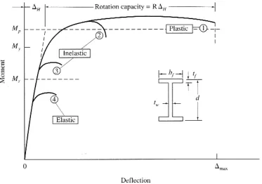
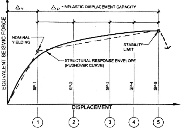
Fig. 2.1-1 shows a complete system force-displacement graph from which all codified seismic design principles, including limit states, are based.

Figure 2.1-1. System force-displacement graph (Uang, 1991)

(46)

13

the structural integrity of a system at various stages along the force-displacement curve. The proposed limit states are defined in Table 2.1-1 and graphically represented in Fig. 2.1-2.

Performance Level Qualitative Description Definition

SP-1 Operational (Service) Yield mechanism; damage is _negligible

SP-2 Occupiable Damage is minor to moderate;

some repair is required

SP-3 Life Safe Damage is moderate to major; _{extensive repairs are required}

SP-4 Near Collapse Damage is major; repairs may _{be uneconomically feasible}

SP-5 Collapse Collapse is imminent

Table 2.1-1. Structural Performance Levels (SEAOC Blue Book, 1999)

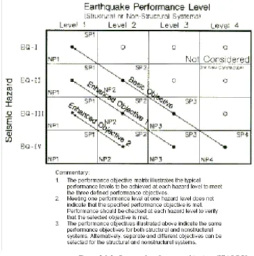
Figure 2.1-2. Graphical representation of structural performance levels

(SEAOC Blue Book, 1999: modified: Harris)

(47)

14

The design engineer selects the design performance objective of the system in accordance with damage level requirements and assigns earthquake levels, based on mean return period and annual probability of exceedance, to each respective performance level.

Figure 2.1-3. Structural performance objectives (SEAOC Blue Book, 1999)

(48)

15

For this research the Basic Safety Objective (BSO) is selected, hence, the performance levels with associated earthquake levels are indicated in Table 2.1-3.

Performance Level Earthquake Level

SP-1 EQ I

SP-2 EQ II

SP-3 EQ III

SP-4 EQ IV (MCE)

Table 2.1-3. Basic safety performance objective

In truth, the design engineer can associate any earthquake level with any performance level. For example, if the system were required to remain “operational” (SP-1) at the maximum considered earthquake (MCE), then EQ IV would be associated with the SP-1 performance level. Hence, all other performance and earthquake levels (I, II, and III) can be neglected. Though this example might be uneconomical, it emphasizes that a selected performance level and respective earthquake level are initially independent. As will be shown subsequently, once the controlling design performance level is determined, performance levels and earthquake levels are in fact dependent. This dependence will allow the design engineer to design a system to respond in accordance with the complete performance objective and not just match one performance level (controlling).

In accordance with the current PBSE code, the design engineer constructs the design response spectrums associated with each earthquake level based on specified effective peak ground accelerations. It should be mentioned that this procedure is slightly revised in this document as discussed in Section 2.5.

(49)

16

2.1.1 Ductility

Ductility, µ, represents a damage level indicator and can be quantified by the ratio of response to yield response. This response action can be measured by section curvature, member rotation, element strain, or displacements. However, these ductility actions typically do not generate the same results. That is curvature ductility will not equal displacement ductility. Though it is assumed by current seismic codes that displacement ductility is equal to rotation ductility, which is similarly equivalent to the force reduction factor, R, employed in force-based design. Since displacements are the easiest form of measurement for the design engineer to visualize and evaluate, it is the preferred choice of ductility measurement and the main quantifier in displacement-based seismic design.

y ∆

∆ =

∆

µ (2.1-1)

where

y

∆ = Yield displacement (in, mm)

Prior to discussing the global design procedures encompassing DBD once the performance objective has been selected, the relationship between member and system response needs to be addressed. That is section curvature and member rotation play an important role in predicting the global response of a system subjected to strong ground motion and, ultimately, the quantitative measure of the frame ductility capacity.

2.2 Section

Curvature

2.2.1 Yield Curvature

From mechanics, the section curvature, φ, for a beam subjected to a bending moment about the major centroidal axis is defined as

x EI

M

=

(50)

17 where

M = Applied moment (k in, N mm)

E = Nominal Modulus of Elasticity (ksi, MPa)

Ix = Moment of Inertia about the major centroidal axis (in4, mm4)

Evaluating Eq. (2.2.1-1) at full yield (i.e. all extreme compression and tension fibers are yielding), we have

x y y

EI M

=

φ (2.2.1-2)

where

My = Section yield moment capacity (k in, N mm)

Eq. (2.2.1-2) can be further expanded using the following known classical relationships.

y o m x y S F

M = φ (2.2.1-3)

2

d

y_o = (2.2.1-4)

o x x

y I

S = (2.2.1-5)

E F_y y =

ε (2.2.1-6)

where

Sx = Elastic section modulus (in3, mm3)

Fy = Nominal yield stress (ksi, MPa)

(51)

18

d = Depth of section (in, mm)

εy = Nominal yield strain from Hooke’s Law

o m

φ = Material overstrength factor (discussed in Section 2.2.5)

Substituting Eqs. (2.2.1-3) through (2.2.1-6) into Eq. (2.2.1-2), the section curvature of an element subjected to pure bending at yield is

d EI F S EI M y o m x y o m x x y y ε φ φ

φ = = = 2 (2.2.1-7)

Evaluation of Eq. (2.2.1-7) shows that the yield curvature is dependent only on section geometry, independent of strength (Priestley and Kowalsky, 2000). Furthermore, evaluation of Eq. (2.2.1-1) in the whole range of member behavior concludes that stiffness is proportional to strength. The proportionality between strength and stiffness contradicts the FBD assumption that an initial stiffness, and, ultimately, the elastic system period, can be determined independent of strength. That is the action of allocating strength between members also changes the stiffness from the initial assumption, and, hence, implies an iterative analysis procedure (Priestley and Kowalsky, 2000). Furthermore, the determination of a non-dimensional section yield curvature indicates that the yield drift of frames might possess the same independence (Priestley, 2000).

2.2.2 Equivalent

Plastic Curvature

Eqs. (2.2.1-1) and (2.2.1-2) outline the moment-curvature relationship of an elastic section represented by the straight line in Fig. 2.2.2-1. Post-yield section curvatures can be determined by Eq. (2.2.2-1) and similarly graphed in Fig. 2.2.2-1.

y y

F M

S

M _

            − = 2 3 1 1 φ φ (2.2.2-1) where

(52)

19

Figure 2.2.2-1. Normalized moment-curvature graph (Chen et al, 1995: modified: Harris)

Due to the iterative nature of an exact non-linear analysis, the bi-linear idealization, shown in Figure 2.2.2-2, is recommended for its simplicity. In this elasto-perfectly plastic idealization, the element is assumed to behave elastically up to the plastic moment, where all plastic rotations occur at a zero length plastic hinge and the plastic curvature increases indefinitely with constant plastic moment capacity (Chen et al, 1995)

Figure 2.2.2-2. Elasto-perfectly plastic moment-curvature graph

(53)

20

This idealization results in a considerable simplification of the analysis procedure without significant compromise in the accuracy of the computed plastic limit load (Chen et al, 1995).

Similar to the previous derivation of the section yield curvature, we substitute Eqs. (2.2.2-2) and (2.2.2-3) into Eq. (2.2.1-1).

y o m x p Z F

M = φ (2.2.2-2)

x x F _S

Z

S = (2.2.2-3)

where

Mp = Section plastic moment capacity (k in, kN mm)

Zx = Geometric plastic section modulus (in3, mm3)

Hence, the equivalent plastic section curvature in accordance with the bi-linear approximation, represented by point A in Figure 2.2.2-2, can be expressed as

d d

S EI

M o _y

m y

o m F

x p p

ε φ ε

φ

φ = = 2 ≈ 2.28 (2.2.2-4)

The shape factor, SF, for North American wide flange sections can be approximated as 1.14

in lieu of the actual value. However, in some cases it will be necessary for the design engineer to include a modification factor during the member design stage representing the ratio of actual to assumed shape factor, discussed subsequently in Section 2.4.6. Again, it shall be emphasized that Eq. (2.2.2-4) is the equivalent plastic section curvature of an element subjected to pure full plastic bending (i.e. no axial load effects). Furthermore, the

equivalent plastic section curvature replaces the yield curvature, φ_y, in the determination of curvature ductility.

p φ

φ

(54)

21

2.2.3 First-Yield Curvature

An additional curvature that needs to be discussed is the curvature at first-yield. As a result of the cooling process steel inherently contains residual stresses. The magnitude of these stresses varies depending on section geometry. Fig. 2.2.3-1 shows an example of residual stress distribution and its effect on the behavior of a wide-flange section.

Figure 2.2.3-1. Flexural behavior of wide-flange with residual stresses (Uang et al, 1998)

In accordance with AISC specifications, the design magnitude of compressive residual stresses, Fr, is shown in Table 2.2.3-1.

Fy Fr Ratio

36 ksi (250 MPa) 10 ksi (69 MPa) 0.72 50 ksi (345 MPa) 16.5 ksi (114 MPa) 0.67

Table 2.2.3-1. Recommended design magnitude of compressive residual stresses (AISC)

Similar to the previous derivations,

L o m x r S F

M = φ (2.2.3-1)

E F_L y' =

(55)

22

y

y ε

ε _' ≈0.7 (2.2.3-3)

where

Mr = Section elastic moment capacity at first-yield (k in, kN mm)

FL = Fy - Fr (ksi, MPa)

Fr = Nominal compressive residual stress (ksi, MPa)

'

y

ε = Nominal first-yield strain from Hooke’s Law

Hence, the section curvature at first-yield can be expressed by

d d

EI

M mo y mo y

x r y

ε φ ε

φ

φ 2 ' 1.4

' = = ≈ (2.2.3-4)

Although, residual stresses can be large, they have no impact on the plastic moment capacity of a section (Uang et al, 1998)

2.2.4 Curvature Reduction for Combined Load Effects

2.2.4.1 Reduction for Axial Compression

The previous sections derived the section curvature of an element subjected to pure bending. However, the application of an axial force affects the yield curvature by reducing the allowable magnitude of the applied moment. From mechanics, the stress distribution for a member subjected to combined loading is

g x A

P S

M _±

=

σ (2.2.4.1-1)

For axial compression, the stress at the extreme compression fiber at yield is

y g x

c F

A P S

M ₊ ₌

=

(56)

23

Similarly, at the extreme tension fiber, the flexural stress from Eq. (2.2.4.1-2) is

g y x t A P F S

M ₌ ₋

=

σ (2.2.4.1-3)

Substituting Eq. (2.2.4.1-3) into Eq. (2.2.4.1-1), we have

g y g g y g x t _A P F A P A P F A P S

M ₋ ₌ ₋2

        − = − =

σ (2.2.4.1-4)

Applying

y g y A F

P = (2.2.4.1-5)

the resulting tensile stress can be expressed as

        − = − = − = y y y y y g y t P P F P PF F A P

F 2 2 1 2

σ (2.2.4.1-6)

Since the overstength factor, o m

φ , is included in the final curvature calculation, it should not be additionally included in the previous equations.

Applying Hooke’s Law and evaluating the strain distribution, we have from similar triangles

c d P P c y y y −         − = 2 1 ε ε (2.2.4.1-7)

Solving Eq. (2.2.4.1-7) for c, the distance from the extreme compression fiber to the neutral axis, we have

(57)

24 By trigonometry and including o

m

φ to denote the variation in material strength, the section yield curvature for a member subjected to bending and an axial force can be expressed as

        − = y y o m y _P P d 1

2φ ε

φ (2.2.4.1-9)

It can be seen from Eq. (2.2.4.1-9) that the reduced yield moment capacity is dependent on the magnitude of axial load and can be expressed as

y y

yc M

P P

M _

      −

= 1 (2.2.4.1-10)

It should be mentioned, as similar notations will be used subsequently, that the 2nd subscript denotes the load effect causing the reduction.

Similarly, the equivalent plastic and first-yield curvatures become respectively

        − ≈         − = y y o m y y o m F p P P d P P d S 1 28 . 2 1

2 φ ε φ ε

φ (2.2.4.1-11)

        − ≈         − = y y o m y y o m y P P d P P d 1 4 . 1 1 2 _' ' ε φ ε φ

φ (2.2.4.1-12)

The reduced plastic moment capacity can similarly be expressed by Eqs. (2.2.4.1-13) and (2.2.4.1-14) and graphically shown in Fig. 2.2.4.1-1.

For 0≤P≤0.15P_y

p pc M

M = (2.2.4.1-13)

For 0.15P_y ≤P≤P_y

p y

pc M

P P

M _

      −

Seismic Analysis and Design of Type FR Steel Frames Using Displacement-Based Design and Advanced Analysis

Abstract

SEISMIC ANALYSIS AND DESIGN OF TYPE FR STEEL

FRAMES USING DISPLACEMENT-BASED DESIGN AND

ADVANCED ANALYSIS

Unquestioned answers are more dangerous than unanswered questions

Unknown

Dedicated to

Biography

Acknowledgements

Table of Contents

List of Tables

List of Figures

List of Symbols

List of Abbreviations

PART 1

I

I

N

N

T

T

R

R

O

O

D

D

U

U

C

C

T

T

I

I

O

O

N

N

,

,

S

1.0 Introduction

1.1 Current

Research

1.2 Simplifications, Assumptions, and Constant Variables

1.2.1 Simplifications

1.2.2 Assumptions

1.2.3 Constant Variables

PART 2

D

2.0 Introduction

2.1 SEAOC Specification for Performance-Based Design

2.1.1 Ductility

2.2 Section

Curvature

2.2.1 Yield Curvature

2.2.2

Equivalent

Plastic Curvature

2.2.3 First-Yield Curvature

2.2.4 Curvature Reduction for Combined Load Effects