ABSTRACT
TOUMA, DANIELLE ELIE. A Quantitative Framework for Assessing the Effects of Climate and Land-use Change on Streamflow. (Under the direction of Dr. Ranji Ranjithan, Dr. E. Downey Brill and Dr. Sankar Arumugam.)
The objective of this research was to develop and test a framework that can be used to assess the effects of climate and land-use change on the stream ecology in a basin. The current method of analyzing extreme events of streamflow is insufficient in non-stationary environments. Although tools and models are available for this assessment, no systematic approach is established. The proposed framework outlines and integrates the key steps and necessary procedures to assess the changes in streamflows. Precipitation and temperature data from four General Circulation Models (GCMs) and land cover data from a land-use model were coupled with a hydrologic model to simulate daily flows. The GCM monthly precipitation and temperature data were preprocessed using a downscaling method to achieve data on a refined spatial scale and a k-Nearest Neighbor algorithm was used to temporally disaggregate the data to a daily scale. The housing density data from the EPA Integrated Climate and Land-use Scenarios (ICLUS HD) were reclassified to be compatible with the USGS National Land Cover Database. The Soil and Water Assessment Tool (SWAT) was used to process the land-use and climate data in the basin. The flow values were used to estimate several Indicators of Hydrologic Alteration (IHA) which were then assessed for the amount of changes using the Range of Variability Approach (RVA). The hydrologic
alterations are evaluated based on flows in a pre-development period and post-development period. To assess the changes under reduced scenario uncertainties and realistic planning time frames, the post-development period flows were scenario simulated for 2011-2040, while the pre-development period flows were simulated using the observed conditions between 1981-2010.
The North East Cape Fear River basin was used to illustrate the framework. The SWAT model was calibrated to an R2 of 0.69 for the daily streamflow. The A2 and B1 scenarios from the Fourth Assessment Report from the Intergovernmental Panel for Climate Change were used in the framework to drive the climate and land-use changes in the
precipitation, 0.35 – 1.10 °C increase in mean temperature based on four different types of GCMs. Urban development is expected to increase by 14 – 17% between the
by
Danielle Elie Touma
A thesis submitted to the Graduate Faculty of North Carolina State University
in partial fulfillment of the requirements for the Degree of
Master of Science
Civil Engineering
Raleigh, North Carolina 2011
APPROVED BY:
______________________ ____________________
Dr. Sankar Arumugam Dr. E. Downey Brill
______________________ Dr. Ranji Ranjithan
DEDICATION
BIOGRAPHY
ACKNOWLEDGEMENTS
I would like to express my gratitude towards my advisor and mentor, Dr. Ranjithan, for allowing me to explore my interests while giving me priceless guidance throughout. He has taught me to always step away and look at the big picture, which is important both in research and in life. I am grateful to Dr. Arumugam who has taught me almost everything I know in Hydrology and introduced me to the issues and research in the field. I would also like to thank Dr. Brill for always provoking me to think about different aspects of the problem.
I am grateful to my Mom and Dad, who have been geographically far but emotionally close and have supported me throughout my life in good and bad times. I am also grateful to my sister, Serene, who kept me fashionable throughout my graduate career and continuously reminded me that what I was doing was valuable by sending me news articles about global water issues. I would like to thank my Raleigh “Mom”, Sirine Schtakleff, who has been my number one support here in NC for six years.
I would like to thank my research group: Linda, Hui and Weihua who have provided me with insightful and helpful research support all the way from calibration to presentation. I wish you all the best in your studies. I would like to thank Brianne and Rachel in Mann Hall who have never let me down when I needed help administratively. I would also like to thank the graduate students in Mann Hall who ultimately became my friends.
I would like to thank my friends in Raleigh who have supported me throughout my studies. Thanks for making even the worse days fun. Thanks to Kurt, not only for buying me a coffee-maker, but also for being my constant and best friend for the last year.
TABLE OF CONTENTS
LIST OF TABLES ... vii
LIST OF FIGURES ... viii
1. Introduction ... 1
2. Problem definition ... 2
3. Methodology ... 4
3.1. Climate data... 5
3.1.1. Spatial downscaling ... 6
3.1.2. Temporal disaggregation ... 7
3.2. Land-use data ... 8
3.3. Hydrologic watershed model ... 9
3.4. Assessment of flows ... 10
3.4.1. Statistical approach ... 11
3.4.2. Ecological flow alterations analysis... 12
4. Illustrative example ... 16
4.1. Basin description ... 16
4.2. Calibration of the SWAT model for the NECF basin ... 19
4.3. Future climate and land-use change in the NECF River Basin ... 22
4.3.1. Projected climate change in the NECF River Basin ... 22
4.3.2. Future land-use changes in the NECF River Basin ... 26
5. Results and discussion ... 29
5.1. Results from the illustrative example ... 29
5.1.1. Statistical analysis of flows ... 29
5.1.3. General observations from the illustrative application ... 40
5.2. Discussion of framework ... 41
6. Concluding remarks ... 43
LIST OF TABLES
Table 2.1: Descriptions of the A2 and B1 storylines from IPCC AR4. ... 3
Table 3.1: EPA ICLUS HD categories' definitions. ... 9
Table 3.2 USGS NLCD 2001 class definitions. ... 9
Table 3.3: Combinations for the post-development period flows... 11
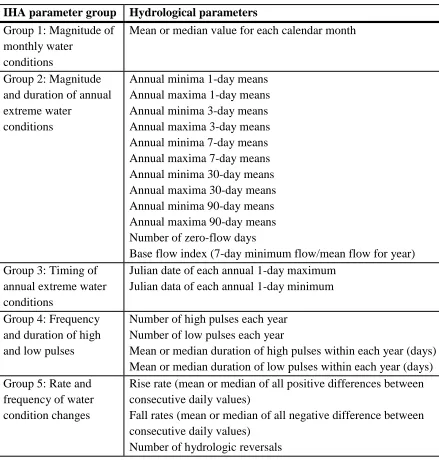
Table 3.4: Summary of IHA parameters as classified into five groups. ... 14
Table 3.5: Sum of mis-hits and alteration ratio calculations for the example in Figure 3.2. .. 16
Table 4.1: NCLD 2001 Land-use/Land Cover categories in the basin with the corresponding percentage of basin area covered. ... 18
Table 4.2: Statistics of SWAT model calibration using 1981-2005 observations at the NECF outlet. ... 20
Table 4.3: Mean annual precipitation in the basin for the A2 and B1 scenarios. Values that are significantly different than the pre-development period values are indicated by an asterisk. ... 22
Table 4.4: Statistical properties of the temperature for the basin for the A2 and B1 scenarios ... 25
Table 4.5: Average growth over the continental US in the Urban/Suburban and Commercial/Industrial categories for the two scenarios. ... 27
LIST OF FIGURES
Figure 2.1: Emissions and population projections for the A2 and B1 storylines (SRES, 2000). ... 3 Figure 3.1: Structure of the framework used for assessing the impact of climate change and land-use change on ecological flows. ... 5 Figure 3.2: 3-Day Maximum analysis for an example set of pre-development period and post-development period flows. ... 15 Figure 3.3: Graphical representation of alteration ratio. Dashed triangle shows the
Figure 5.5: Hydrologic alteration ratios for the maximum flow (IHA Group 2) parameters estimated using the (a) ECHAM-based flow simulations for the A2 scenario and (b) using the CCSM-based flow simulations for the A2 scenario. ... 35 Figure 5.6: Hydrologic alteration ratios for the maximum flow (IHA Group 2) parameters estimated using the CCSM-based flow simulations for the B1scenario. ... 35 Figure 5.7: Group 1 of IHA parameters' alteration ratios for the CCSM simulation for the A2 scenario. ... 36 Figure 5.8: Group 1 of IHA parameters' alteration ratios for the CCSM simulation for the B1 scenario. ... 37 Figure 5.9: Mean monthly flows (IHA Group 1) alteration ratios for the A2 scenario for land-use change alone. ... 38 Figure 5.10: Mean monthly flows (IHA Group 1) alteration ratios for the B1 scenario for land-use change alone. ... 38 Figure 5.11: Annual minimum flows (IHA Group 2) alteration ratio for (a) A2 and (b) B1 scenarios for land-use change alone. ... 39 Figure 5.12: Annual maximum flows (IHA Group 2) alteration ratio for (a) A2 and (b) B1 scenarios for land-use change alone. ... 39 Figure 5.13: Average sum of mis-hits over all GCM flow simulations for Group 1 and Group 2 of the IHA parameters. ... 40 Figure 5.14: Total sum of mis-hits for Group 1 and Group 2 of IHA parameters for the A2 and B1scnearios for all GCM flow simulations. ... 41 Figure 5.15: Mean annual changes of precipitation and temperature between 1970-1999 and 2010-2039, 2040-2069 and 2070-2099 for raw GCM data, bias-corrected data and
1.
Introduction
The hydrology in a watershed can be impacted by changes in land-use and climate. These changes can ultimately affect the ecology by altering the flows in the channel. Assessments of these effects have been studied for at least two decades, and a large number of hydrologic, climate and land-use models have been developed. National datasets have also been
established ranging from observed hydroclimatic time series to future scenarios of the climate that are provided by the Intergovernmental Panel for Climate Change (IPCC). The common practice related to development in watersheds, however, continues to focus on analyzing the peak flow of extreme events and minimum flows. This has been criticized as being insufficient in a non-stationary environment and for ecological purposes (Poff et al., 1997).
Studies in the past have assessed streamflow changes in the watershed due to either climate change, land-use change, or both, but there is no established approach to study these changes systematically. Basins have been studied using different methodologies, resulting in different types of results. Praskievicz and Chang (2009) summarize multiple studies that have assessed the changes in streamflow due to climate or land-use change. Consideration of uncertainties includes scenario uncertainty, model uncertainty and variability in the associated physical (e.g., atmospheric and hydrological) systems (Hawkins and Sutton, 2009; Praskievicz and Chang, 2009).
monthly flows influence the habitat availability for aquatic organisms and the reliability of water supplies for terrestrial animals, while the timing of extreme annual conditions is linked to the life cycle of organisms as well as their reproduction needs. Some other flow
parameters represent nutrient and organic matter availability and drought stress on plants. The IHA parameters also capture common hydrologic characteristics of the flow regime that are studied for other applications such as reservoir management and water treatment (Richter, 1996). These parameters can be used to establish a systematic approach within a quantitative framework to assess the effects of climate and land-use change scenarios on streamflow and associated ecological impacts.
This paper describes a framework for analyzing the impacts of climate change and land-use change on ecological flow alterations in a basin. First, the climate and land-use changes that are being assessed are described, including their temporal and spatial scales. Then, the models used in the framework as well as the available data sets are presented. Subsequently, the study applies the framework to assess a basin in North Carolina that has been
experiencing rapid development. Then the results from the analyses are presented, with a discussion of the impacts of climate and land-use changes in altering ecological flows. Finally, concluding remarks and observations about the framework are presented.
2.
Problem definition
This paper provides a framework for assessing the role of climate and land-use changes in altering the ecological flow in a basin. Future changes in the climate and land-use are uncertain since they depend on the economy, politics and demography of the globe. As the lead-time increases, future projections deviate further from the present and more assumptions are made, and become more uncertain. Therefore, it is important to consider different
projections as characterized by the storylines developed by the Intergovernmental Panel for Climate Change (IPCC) to assess the changes in a basin. Storylines A2 and B1 are
Table 2.1: Descriptions of the A2 and B1 storylines from IPCC AR4.
A2 B1
Differentiated world Convergent world
Regionally oriented economy with a lowest per capita growth out of all scenarios
Service and information based economy with a higher per capita growth than A2 but not the highest
Continuously increasing population Population peaks at 2050 then declines Self-reliant governments preserve local
identities
Global governments provide solutions to economic, social and environmental sustainability
Slowest and most fragmented technological development out of all scenarios
Clean and resource efficient technologies
To make these storylines more relevant and meaningful, they have been converted to scenarios that project the changes in populations, GDP, land development, emissions and other parameters related to growth (Figure 2.1). The scenarios can then be explicitly
incorporated to drive the emissions in general circulation models (GCMs) and the associated land development in land-use models. Using this information, assessments can be made about other aspects of the physical environment, including the hydrological and ecological impacts in the basin.
Figure 2.1: Emissions and population projections for the A2 and B1 storylines (SRES, 2000).
later years (100 years) (Hawkins and Sutton, 2009). Engineering and planning decisions typically take place in this time frame. Having a more reliable and realistic assessment for the next 30 years is more helpful and needed than a vague vision for the next 100 years. Therefore, the analysis presented is illustrated using a near-term (30 years) consideration, even though it could be used over other desired time scales.
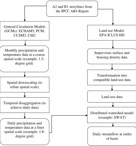
Data from GCMs and the Environmental Protection Agency (EPA) Integrated Climate and Land-Use Scenarios (ICLUS HD) (US EPA, 2009) for the A2 and B1 storylines are
combined with a hydrologic watershed model. Using demographic population projections consistent with the storylines as an input, the ICLUS HD model assigns new housing densities across the landscape (US EPA, 2009). Because the available climatic data are not spatially or temporally compatible with the hydrologic model, several preprocessing steps are used in the framework. This includes spatio-temporal downscaling of climatic data so that it can be utilized as daily input into the watershed model, and conversion from housing density classes into National Land Cover Data set classes to correctly model the hydrologic
processes. By matching the climate and land-use data to the spatio-temporal resolution of the watershed model, changes in the streamflows can then be assessed using flow regime
alteration indicators represented by the IHA parameters and other statistical measures.
3.
Methodology
3.1.
Climate data
Sixteen GCM model simulations for the A2 and B1 scenarios are available from the IPCC database for the years 2010-2100. The models chosen in this study are ECHAM 5 (Jungclaus et al., 2006) by the Max Planck Institute for Meteorology, CM2.0 (Delworth et al., 2005) by Figure 3.1:Structure of the framework used for assessing the impact of climate change and land-use change on ecological flows.
A2 and B1 storylines from the IPCC AR4 Report
General Circulation Models (GCMs): ECHAM5, PCM,
CCSM3, CM2
Land-use Model: EPA ICLUS HD
Monthly precipitation and temperature data at a coarse
spatial scale (example: 1.5-degree grid)
Spatial downscaling (to refine spatial scale)
Impervious surface and housing density data
Transformation into compatible land-use data
Daily precipitation and temperature data at a finer spatial scale (example:
1/8-degree grid)
Temporal disaggregation (to achieve daily data)
Land-use data
Distributed watershed model (example: SWAT)
the Geophysical Fluid Dynamic Laboratory, NOAA, and the PCM (Washington et al., 2000) and CCSM3 (Collins et al., 2006) by the National Center for Atmospheric Research. These models have been used often for impact studies in the US and are generally accepted in the climate and hydrological modeling communities. Projections from these GCMs, primarily precipitation and temperature, are available at a monthly time scale over a larger spatial resolution.
3.1.1. Spatial downscaling
The spatial scale of the climate data, which is in a 1.5-degree grid, has large biases in certain geographic areas, especially in coastal or mountainous regions (Wood et al., 2002). To overcome this issue, regional climate models can be used, but they are computationally intensive. Therefore, spatial downscaling using statistical techniques was used in the
framework to obtain the climate data in a 1/8-degree grid scale. Spatial downscaling requires observed data for both 1/8-degree and 1.5-degree scales. Additionally, GCM-simulated climate data for the observed period is needed. The observed data on a daily scale is available from the Surface Water Modeling group at the University of Washington for the US (Maurer et al., 2002). The GCM’s historical predictions are also available from the IPCC database.
CMIP3 maintains a database for the sixteen climate models with downscaled datasets of monthly precipitation and temperature at a 1/8-degree grid for the US. These datasets were used in the research reported here.
3.1.2. Temporal disaggregation
For the purpose of simulating the hydrologic model at a daily scale, temporal disaggregation was applied to obtain daily precipitation and temperature data from the GCMs’ monthly data. A k-nearest-neighbor algorithm (k-NN) was used to temporally disaggregate the downscaled monthly climate data (Cover and Hart, 1967). This disaggregation method was used in the studies reported by both Wood et al. (2002) and Salathe (2004). This method uses past daily observations to create the structure of the daily temperature and precipitation data based on the future monthly values, assuming that the daily structure is similar. Also, each month was disaggregated using the values for the same month from the historic data. For example, to disaggregate the monthly precipitation value for January 2015, only January historic data were used. This approach preserves the seasonality with the associated climate data. The closest neighbor was used to disaggregate precipitation to preserve the number of zero-rain days. The observed and future monthly time series of the grid points in the basin were spatially averaged. Then, for each spatially averaged future month, a nearest neighbor month was chosen from the spatially averaged observed data. Then, this nearest neighbor month was used to disaggregate all the grid points in the future month. The daily precipitation values from the nearest neighbor month were divided by the total precipitation of that month to obtain daily fractions. Each daily fraction was then applied to the future monthly value to obtain daily time series of precipitation under different scenarios.
(3.1) where w(k) is the weight of the kth neighbor.
The minimum and maximum temperatures for each day of the future month were obtained by using a weighted average of the observed minimum and maximum temperatures in the
neighboring months.
3.2.
Land-use data
Land-use data for the framework (Figure 3.1) were obtained from two sources: the current land-use data were obtained from the 2001 USGS National Land Cover Database (NLCD 2001) (USGS, 2008) and the land-use model projections for housing density scenarios were obtained from EPA’s ICLUS HD (US EPA, 2009). The ICLUS HD scenarios are available on a decadal scale for the 21st century on a one-hectare scale for all of the US. The land-use models are also available as ArcGIS toolboxes in which the parameters can be modified to specify different scenarios.
There is incompatibility between the NLCD 2001 and ICLUS HD datasets due to the different land-use classifications. The ICLUS HD categories are rural, exurban,
Table 3.1: EPA ICLUS HD categories' definitions.
Housing density category EPA definition (lots/acre) Rural >16.18 ha per housing unit (<0.03) Exurban 0.68-16.18 ha per housing unit (0.03-0.60) Urban/Suburban < 0.68 ha per housing unit (>0.6) Commercial/Industrial > 25% urban/built up areas Table 3.2 USGS NLCD 2001 class definitions.
NLCD 2001 class Definition SCS curve number description Developed, Low intensity Single family housing units 1 lot/acre Developed, Medium intensity Single family housing units 2-4 lots/acre
Developed, High intensity Apartment complexes, row houses 8 lots/acre Industrial Infrastructure, highly developed 80% impervious By doing an assessment of the relationship between the lot/acre measure in the ICLUS HD definition and the SCS curve number descriptions of the NLCD 2001 class, all the
“developed” NLCD 2001 classes were found to fit the definition of the Urban/Suburban EPA category. Therefore, the growth in the Urban/Suburban category was applied equally to the NLCD developed classes, and the growth in the Commercial/Industrial category was applied to the industrial NLCD 2001 class. Even though this simplifies the relationship, it captures the average development that occurs in the basin.
Additionally, the ICLUS HD project output does not specify the changes by the land-use categories, but by urban density changes. Thus, an assumption must be made about the other land-uses in the basin. Possible sources of information to improve these assumptions include local or regional planning documents.
3.3.
Hydrologic watershed model
the water balance in the watershed, taking into account the climate, the topography, soil and land-use in the watershed. The SWAT model splits the basin into several subbasins, which are then split into hydrologic response units (HRUs) that have their unique land-use, soil type and slope specifications. HRUs are not allocated spatially in the subbasin, but are
computational units that are used to calculate mass balances for the subbasin. Using the HRUs, the land phase of the hydrologic cycles is processed to determine the amount of water as well as nutrient and sediment loadings to the subbasin channel. The routing phase of the hydrologic cycle then moves the water through the channel network in the watershed to the basin outlet (Neitsch et al., 2005). Land-use can be allocated on a subbasin-specific scale, which is acceptable for smaller watersheds.
The SWAT model is available in ESRI ArcMap, which is part of the ArcGIS Desktop package, through an interface developed by Blackland Research Center in the Texas Agricultural Experiment Center (Winchell at al., 2010). The ArcSWAT interface within ESRI ArcMAP analyzes the topography and allows for an outlet to be chosen within the basin for automatic watershed delineation. The topography is represented by the Digital Elevation Model (DEM), which was obtained from the USGS Seamless Server (USGS, 2004). Additionally, soil data were retrieved from the National Resources Conservation Service (NRCS) (Soil Survey Staff, 2010), which is part of the Department of Agriculture. These are raster datasets with the DEM being on a refined 1/3-degree scale.
3.4.
Assessment of flows
The output of the framework is the time series of daily flows at the outlet of the basin (Figure 3.1), which was then processed using statistical methods to assess changes in the flow
For the pre-development period data, the model was run using the NLCD 2001 land-use cover set, and the flow was simulated using the observed gridded precipitation and
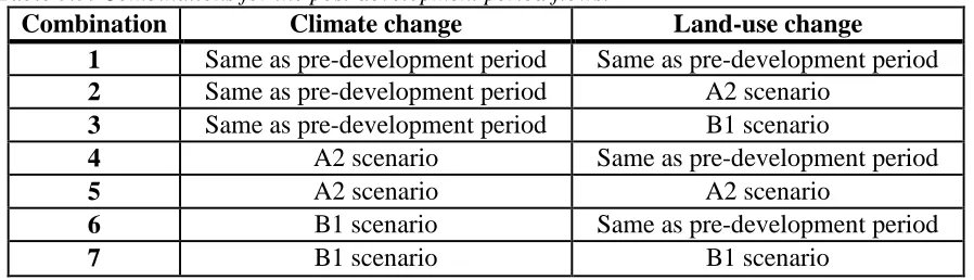
temperature data. The post-development period was based on seven combinations, in which the climate and land-use change data for different scenarios was used (Table 3.3). These combinations are realistic possibilities for the future and are useful in separating the land-use change effects from the climate change effects. The model was run continuously from 1980-2040, and the land-use for 2020 and 2030 was updated accordingly for Combinations 2, 3, 5 and 7. To assess the changes between the two periods using a statistical approach,
significance testing of the changes in mean, standard deviation and trends of streamflow was conducted.
Table 3.3: Combinations for the post-development period flows.
Combination Climate change Land-use change
1 Same as pre-development period Same as pre-development period
2 Same as pre-development period A2 scenario
3 Same as pre-development period B1 scenario
4 A2 scenario Same as pre-development period
5 A2 scenario A2 scenario
6 B1 scenario Same as pre-development period
7 B1 scenario B1 scenario
3.4.1. Statistical approach
Significance tests are used to verify whether any change between the pre-development period and post-development period is a sampling error or a meaningful change. The two-sample t -test was used to -test whether the differences in the mean flow values are statistically
significant:
(3.2)
where the pooled variance, is defined as
where is the mean of the variable in the pre-development period, is the mean of the variable in the post-development period, is the variance of the variable in the pre-development period, is the variance of the variable in the post-development period, n number of data points in the pre-development period, m is the number of data points in the post-development period, and is the percentile of the t-distribution for α level of
significance and df degrees of freedom (Larsen and Marx, 2006).
The F-test was then used to evaluate the significance of a given change in the variance of streamflow data. Whether there is a change in the mean or not, a change in the annual
variance may denote an alteration in the flow regime between the pre- and post-development periods. For the variance to be significantly different,
, (3.4)
where is the percentile of the F-distribution for α level of significance with m and n degrees of freedom (Larsen and Marx, 2006).
A trend could also be present in the flow, indicating that the flows are consistently increasing or decreasing due to land development. To test for the significance of a trend, a linear
regression equation, y = bt + c, was created. The predictor, t, is time, the predictand, y, is the annual precipitation, temperature or streamflow, and b describes the trend of the variable in time. To show its significance at an α level, a derivation of the t-statistic was used (Larsen and Marx, 2006).
, (3.5)
where is the variance of the data.
3.4.2. Ecological flow alterations analysis
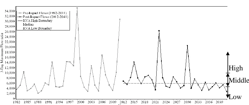
classified into five groups based on their potential effect on the ecology. To assess the relative change in each parameter value, the Range of Variability Approach (RVA) was used (Richter, 1997). The range of variability for each IHA parameter was first obtained by determining the 33rd and 67th percentiles of the flows in the pre-development period. These values define three (high, middle and low) categories in which approximately a third of the data points lie (Figure 3.2). The same distribution is expected to occur in the
Table 3.4: Summary of IHA parameters as classified into five groups.
IHA parameter group Hydrological parameters Group 1: Magnitude of
monthly water conditions
Mean or median value for each calendar month
Group 2: Magnitude and duration of annual extreme water
conditions
Annual minima 1-day means Annual maxima 1-day means Annual minima 3-day means Annual maxima 3-day means Annual minima 7-day means Annual maxima 7-day means Annual minima 30-day means Annual maxima 30-day means Annual minima 90-day means Annual maxima 90-day means Number of zero-flow days
Base flow index (7-day minimum flow/mean flow for year) Group 3: Timing of
annual extreme water conditions
Julian date of each annual 1-day maximum Julian data of each annual 1-day minimum Group 4: Frequency
and duration of high and low pulses
Number of high pulses each year Number of low pulses each year
Mean or median duration of high pulses within each year (days) Mean or median duration of low pulses within each year (days) Group 5: Rate and
frequency of water condition changes
Rise rate (mean or median of all positive differences between consecutive daily values)
Fall rates (mean or median of all negative difference between consecutive daily values)
Figure 3.2: 3-Day Maximum analysis for an example set of pre-development period and post-development period flows.
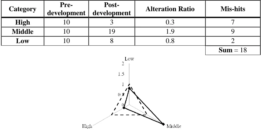
To obtain the total alteration in the variability in all parameter values, the sum of mis-hits approach was used (Table 3.5) (Pierpont, 2008). This approach sums the absolute difference between the pre-development period and the post-development period data points in each category over all the parameters of importance. This approach helps to gain insight into the magnitude of the total change in the parameter values but it does not distinguish the changes by categories or the direction of changes. Thus, an “alteration ratio” was defined to represent the change in relation to the pre-development conditions in each category (Table 3.5 and Figure 3.3). For each parameter, a ratio value of 1 for a category indicates that there is no change in the number of occurrences in that category, while a ratio greater than 1 indicates an increase in the occurrences in that category and vice versa. While this representation of changes in the flow enables assessment of the direction of change as well as the degree of change for each parameter, it is not suitable for an aggregate indicator, which is captured by the number of mis-hits.
Table 3.5: Sum of mis-hits and alteration ratio calculations for the example in Figure 3.2.
Category Pre-development
Post-development Alteration Ratio Mis-hits
High 10 3 0.3 7
Middle 10 19 1.9 9
Low 10 8 0.8 2
Sum = 18
Figure 3.3: Graphical representation of alteration ratio. Dashed triangle shows the no-alteration case while solid line shows the alteration ratios for the 3-Day Maximum Flow parameter illustrated in the example in Figure 3.2.
4.
Illustrative example
4.1.
Basin description
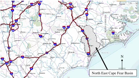
Figure 4.1: Location of NECF River Basin in NC.
Figure 4.2: DEM of the delineated watershed with 23 subbasins, main and tributary reaches and the longest path of flow for each subbasin, calculated by ArcSWAT. The outlet is located on the southern boundary of the basin.
N
North East Cape Fear Basin
Subbasin boundary Reach
The DEM and land-use data were downloaded from the USGS Seamless Server and the soil cover from NRCS (Figures 4.3 a and b). The basin has a relatively low percentage (4.07%) of developed urban area (Table 4.1), but that area is expected to grow in the future decades, as evidenced by the high population growth (in the period 1990-2000) of the two main counties, Pender and Duplin, in the basin with 42% and 23% growth rates, respectively.
a) b)
Figure 4.3: Land-use data (a) from NLCD 2001 data and soil data (b) from NRCS for the NECF Basin.
Table 4.1: NCLD 2001 Land-use/Land Cover categories in the basin with the corresponding percentage of basin area covered.
NCLD 2001 Land-use/Land Cover (abbreviation in legend for Figure 4.3)
Percentage of Basin Area (%)
Water (WATR) 0.18
Residential – Low Density (URLD) 3.28
Residential – Medium Density (URMD) 0.68
Residential – High Density (URHD) 0.09
Industrial (UIDU) 0.02
Forest – Deciduous (FRSD) 3.17
Forest – Evergreen (FRSE) 17.32
Forest – Mixed (FRST) 6.13
Range – Brush (RNGB) 5.50
Range – Grasses (RNGE) 8.66
Hay (HAY) 0.99
Agricultural Land – Row Crops (AGRR) 36.60
Wetlands – Forested (WETF) 16.68
As the simulated climate data for the coastal basin are more likely to exhibit a bias than those for inland basins, a higher level of spatial refinement of the climate data was needed. Gridded observed daily temperature and precipitation data are available on a 1/8-degree scale, which were used to simulate the flow in the pre-development period and to disaggregate the precipitation for the post-development period (Figure 4.4). The seasonality of the climate is in phase, with the highest temperatures coinciding with the greatest amounts of precipitation. This results in the monthly streamflows being greatest in the winter when precipitations rates are relatively high and temperatures are low. Further, the basin experiences low flows during the spring months due to higher temperatures and lower precipitation.
a) b)
Figure 4.4:a) Nine grid points of precipitation and temperature data used for simulating the flows in the NECF basin, and b) spatially averaged 1980-2010 mean monthly precipitation and temperature values for the NECF basin.
4.2.
Calibration of the SWAT model for the NECF basin
flows will be only minimally impacted since it is reasonable to expect the marginal bias to be similar over the pre-development and post-development periods.
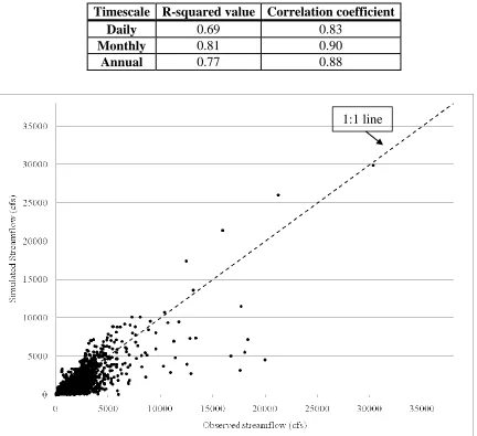
Table 4.2: Statistics of SWAT model calibration using 1981-2005 observations at the NECF outlet.
Timescale R-squared value Correlation coefficient
Daily 0.69 0.83
Monthly 0.81 0.90
Annual 0.77 0.88
Figure 4.6: (a) Mean monthly simulated and observed flows, and (b) mean annual simulated and observed flows for 1981-2005 in the NECF basin.
a)
4.3.
Future climate and land-use change in the NECF River Basin
4.3.1. Projected climate change in the NECF River Basin
The climate data for the basin from the four GCMs that had been spatially downscaled were tested using significance tests described in Section 3.4. Significant changes in the climate data are expected to result in significant changes in the simulated flows. Using the t-test for significance testing, the pre-development period and post-development period mean values were compared for both A2 and B1 scenarios for all GCMs, while the pre-development period and post-development period standard deviations were tested using the F-test. Overall, the mean annual precipitation exhibited significant changes only in two GCMs for the A2 scenario and one GCM for the B1 scenario (Table 4.3).
Table 4.3: Mean annual precipitation in the basin for the A2 and B1 scenarios. Values that are significantly different than the pre-development period values are indicated by an asterisk.
A2 Scenario B1 Scenario
GCM Mean Annual Precipitation Average (mm) Mean Annual Standard Deviation (mm) Mean Annual Precipitation Average (mm) Mean Annual Standard Deviation (mm) Pre-development period
1252 185 1252 185
ECHAM5 1372* 198 1365 348*
PCM 1295 213 1274 214
CCSM3 1352 231 1399* 241
CM2 1388* 246 1349 231
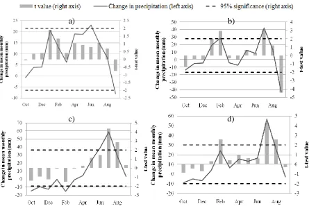
When the monthly means were assessed separately from each other using the t-test, significant changes were seen, however, in the A2 scenario using all GCMs (Figure 4.7). Except for the ECHAM simulation, the significant changes were in February, July and August precipitations. Therefore, these months are expected to show a significant change in the simulated streamflow for the A2 scenario. This implies that the models indicate
Figure 4.7: Changes in the monthly means of the precipitation for the A2 scenario using (a) ECHAM, (b)PCM, (c) CCSM and (d) CM2 data. The t-values are shown for each month with the significant changes showing t-values above the upper or below the lower significance levels.
Unlike in the A2 scenario, the ECHAM model in the B1 scenario had the most number of months with significant changes in the precipitation between pre-development period and post-development period (Figure 4.8a). The PCM, CCSM and CM2 models showed significant increases in the July precipitation values, while a significant decrease was associated with the ECHAM model (Figure 4.8). Additionally, ECHAM and PCM models showed a significant decrease in precipitation in August, but the CCSM and CM2 models showed a significant increase. The variations in the precipitation changes over all the GCMs show the need to use more than one GCM in the framework to overcome the uncertainties among them.
b) a)
Figure 4.8: Changes in the monthly means of the precipitation for the B1 scenario using (a) ECHAM, (b)PCM, (c) CCSM and (d) CM2 data. The t-values are shown for each month with the significant changes showing t-values above the upper or below the lower significance levels.
Based on the t-test and F-test at a 95% significance level, the temperature changes for all GCMs and both scenarios showed no significant changes in the 30-year mean and standard deviation (Table 4.4). Additionally, the trends (not shown here) in both the combined periods and the separate periods were insignificant at a 95% significance level. There were numerous significant monthly changes, however, in the temperature (Figures 4.9 and 4.10). Whether the changes were significant or not in the climate data, the hydrologic aspects of the basin may have been sensitive to the changes and may have resulted in different levels of alteration. Also, the land-use changes may have amplified or subdued the impact of these climate change effects on the basin.
a) b)
Table 4.4: Statistical properties of the temperature for the basin for the A2 and B1 scenarios
A2 Scenario B1 Scenario
GCM Mean
(°C)
Annual Standard Deviation (°C)
Mean (°C)
Annual Standard Deviation (°C)
Pre-development period
16.53 0.678 16.53 0.678
ECHAM5 17.24 0.841 17.24 0.852
PCM 16.88 0.560 17.17 0.486
CCSM3 17.43 0.533 17.63 0.668
CM2 17.26 0.773 17.25 0.666
Figure 4.9: Changes in the monthly means of the temperature for the A2 scenario using (a) ECHAM, (b)PCM, (c) CCSM and (d) CM2 data. The t-values are shown for each month with the significant changes showing t-values above the upper or below the lower significance levels.
b) a)
Figure 4.10: Changes in the monthly means of the temperature for the B1 scenario using (a) ECHAM, (b)PCM, (c) CCSM and (d) CM2 data. The t-values are shown for each month with the significant changes showing t-values above the upper or below the lower significance levels.
4.3.2. Future land-use changes in the NECF River Basin
After having assessed the observed land-use changes in the basin, it was evident that, due to the nature of the basin and the ICLUS HD model, the basin is expected to experience a maximum of only 1% urban growth between 2010 and 2040. Even though this is realistic due to the high level of agricultural activities and presence of wetlands, the future urbanization changes are too low to be assessed. Also, the recent growth rates discussed in Section 4.1 suggest that the basin is expected to grow at a higher rate. Therefore the spatial average of urbanization changes over the US in the ICLUS HD data was applied to this basin (Table 4.5).
b) a)
The A2 scenario showed more aggressive growth in the Urban/Suburban land-use categories while the Commercial/Industrial land-use categories in the B1 scenario grew at a much faster rate. Based on these values, the projected urban areas for both A2 and B1 scenarios are somewhat similar in 2020, but show more variation in 2030 with a greater degree of urbanization in the A2 scenario (Figure 4.11). The future urbanization was introduced by converting range land (RNGE), which is well distributed across the basin and it is not linked to economic activities. Thus, existing urban areas were expanded but no new urban areas were created.
Table 4.5: Average growth over the continental US in the Urban/Suburban and Commercial/Industrial categories for the two scenarios.
A2 Scenario B1 Scenario
Urban/Suburban Commercial/Industrial Urban/Suburban Commercial/Industrial
2020 9.0% 7.7% 8.6% 9.8%
2030 7.3% 7.5% 5.2% 8.2%
Figure 4.11: Projected developed area in the basin for 2020 and 2030 for the A2 and B1 scenarios.
changes decreased between 2020 and 2030, and were not as large as for the A2 scenario (Figure 4.13).
2020 URLD1 URMD RNGE
7 3 -10
4 1 -5
3 1 -4
2 0 -2
2030 URLD URMD RNGE
7 3 -10
4 1 -5
3 1 -4
2 0 -2
Figure 4.12: Percentage changes in the land-use categories in 2020 and 2030 for the different subbasins in the watershed for the A2 scenario that were implemented.
1
5.
Results and discussion
5.1.
Results from the illustrative example
5.1.1. Statistical analysis of flows
The SWAT model was run for 60 years 2040) with the pre-development period (1981-2010) using the observed climate for all grid points and the post-development period (2011-2040) using downscaled and disaggregated data (as described in Section 3.1) from the ECHAM, PCM, CCSM and CM2 climate models. Separate simulations were conducted using each GCM’s climate data and the flow was analyzed at the outlet to the basin (Figure 4.2).
While the climate data showed a lack of significant changes for some of the GCMs, the t-test (Equation 3.2) showed that all the simulated mean daily streamflow values exhibited
increases at a 95% significance level for both A2 and B1 scenarios (Table 5.1). On a daily level, the standard deviations were also significantly different; however, this result may have been due to the high number of degrees of freedom in the F-test calculation (Equation 3.4).
2020 URLD1 URMD RNGE
7 2 -9
4 1 -5
3 1 -4
2 0 -2
2030 URLD URMD RNGE
5 2 -7
4 1 -5
3 1 -4
2 0 -2
Figure 4.13: Percentage changes in the land-use categories in 2020 and 2030 for the different subbasins in the watershed for the B1 scenario that were implemented.
1
These results for the mean and standard deviation show the sensitivity of the hydrological processes to the changes in climate.
Table 5.1: Statistical analysis of the mean daily flow values for the A2and B1 scenario for four GCMs under climate change alone.
A2 Scenario B1 Scenario
GCM Mean
(cfs) Standard deviation (cfs) Mean (cfs) Standard deviation (cfs) Pre-development period
1242 1399 1242 1399
ECHAM 1445 1334 1447 1392
PCM 1313 957 1263 906
CCSM 1415 1329 1476 1277
CM2 1486 1410 1380 1148
Flow duration curves (FDCs) could also be used to analyze the “flashiness” of a basin as well as the behavior of the low flows (Dingman 2008) (Figure 5.1). All FDCs for the A2 scenario (results for only the CCSM model are shown in Figure 5.1) showed an increase in the
Figure 5.1: Flow duration curves for climate change under the A2 scenario using the CCSM climate model for the mean annual flows.
Figure 5.2: Flow duration curves for climate change under the B1 scenario using the CCSM climate model for the mean annual flows.
The t-test was conducted on the mean monthly flow values to check for the significance of the changes in the mean flow at a 95% confidence level. Significant changes in the monthly flow values occurred in the same months for both scenarios for each GCM. This indicates
Pre-development period flows
Post-development period flows
Post-development period flows
that the scenarios are somewhat similar in the near-term since they are dependent on the initial conditions rather than the scenario-relevant factors. Results from the PCM, CCSM, and CM2 models show that the largest increases in mean monthly flows occur in the summer months (results for only the CCSM model for A2 and B1 scenarios are shown in Figure 5.3), while the ECHAM model shows that the most significant increases occur in the winter months. This can be associated with the monthly changes in the precipitation in the basin (Figures 4.7 and 4.8) where the same months show significant increases for each model. For each GCM, the A2 scenario shows an equal or greater number of months with significant changes in the streamflow as the B1 scenario.
Figure 5.3: Changes in mean monthly flows from pre-period to post-period for the CCSM simulation with the t-test value shown in bars for the (a) A2 scenario and the (b) B1 scenario. The change in flow is only significant when the t-test value is greater than the positive 95% significant t-value or less than the negative significant t-value.
The land-use changes in the basin were implemented using the pre-development period (observed) climate data to isolate the flow alterations due to climate change effects from those due to the land-use changes. When the resulting flows were compared to the pre-development period flows corresponding to the current land-use data, no significant changes were observed based on the t-test for the mean and the F-test for the standard deviation. The FDCs for both scenarios also remained unaltered. The impact land-use change has on flow is still an irresolute issue (Praskievicz and Chang, 2000). In some modeling studies, climate change was found to have a greater effect on streamflow than land-use change (Chen et al., 2005; Herron et al., 2002) while the contrary was found in other studies (Chang, 2003; Davis Todd et al., 2007). The former was observed to be the case for this study where the combined
effects of climate change and land-use change on flow were similar to those due to climate change only. The rates of urban growth estimated using the ICLUS HD land-use model for the A2 and B1 scenarios were too low to show any significant alterations. Additionally, retrospective studies have shown that the relative size of the basin influences the effect that urbanization has on the hydrologic cycle (Nirupama and Simonovic, 2007; Wang, 2006).
5.1.2. Ecological assessment of flows
The statistical analysis of the flows described above shows how significant the changes are in the flow but is insufficient to assess the impacts on the ecology of the basin. The IHA
parameters that provide a simple but more comprehensive assessment of the changes in the flows were used to study the changes in flow regimes reflected not only by the magnitude, but also by duration, frequency, and variability of flow.
The FDC curves assessed in Section 5.1.1 identified the increases in the low flows over all the GCMs and scenarios. These changes were assessed in a more comprehensive manner by analyzing the minimum flow parameters in Group 2 of the IHA parameters (Table 3.4). The changes in flows between the pre-development and post-development conditions for the A2 and B1 scenarios were similar, reflected by the increase in occurrences in the high category (upper third percentile) for the minimum flows (Figure 5.5). The A2 scenario showed greater reductions of occurrences in the low category, while the B1 scenario showed greater
Figure 5.4: Hydrologic alteration ratios for the minimum flow (IHA Group 2) parameters estimated using the CCSM-based flow simulations for (a) the A2 scenario and (b) the B1 scenario.
The maximum flow parameters showed larger differences among the GCM model
simulations for the A2 scenario than for the B1 scenario. The ECHAM and PCM simulations showed much greater alterations in flows than those simulated by CCSM and CM2, which showed almost no alterations. Figure 5.5 shows the comparison between ECHAM and CCSM results. Overall, the effects on the maximum flow (IHA Group 1) parameters showed smaller effects compared to those for the minimum flow (IHA Group 2) parameters, as well as showed a tendency for increasing occurrences in the middle category. The GCM
simulations for the B1 scenario showed lower alterations in the maximum flow (IHA Group 1) parameters than for the A2 scenario, with increases in the occurrences in the middle and low flow categories. The results for the CCSM simulations are shown in Figure 5.6.
Figure 5.5: Hydrologic alteration ratios for the maximum flow (IHA Group 2) parameters estimated using the (a) ECHAM-based flow simulations for the A2 scenario and (b) using the CCSM-based flow simulations for the A2 scenario.
Figure 5.6: Hydrologic alteration ratios for the maximum flow (IHA Group 2) parameters estimated using the CCSM-based flow simulations for the B1scenario.
Even though the statistical analysis of the monthly mean flows (Section 5.1.1) show that the changes in monthly flows were only significant in certain months, the IHA Group 1
parameters (Table 3.4) show that all months have alterations with some months showing more than others. The greatest alterations occurred in the same months where significant
changes were seen, but high alterations also occurred where significant changes were not seen. For example, the CCSM simulation of flows for the A2 scenario showed no significant changes in the monthly mean for September (Figure 5.3a); however, the IHA alteration ratios showed a large change in the high category (Figure 5.7). The same was seen for the B1 scenario where the alteration ratio in the high category for October was large (Figure 5.8), but there were no significant changes in the mean flows for that month (Figure 5.3b). These observations show the need to assess the changes in the flows using multiple parameters and methods to correctly analyze the potential effects on ecological flow regimes in the basin.
Figure 5.8: Group 1 of IHA parameters' alteration ratios for the CCSM simulation for the B1 scenario.
Alternatively, there were no alterations in the IHA parameters in Group 1 (Figures 5.9 and 5.10) and Group 2 (Figures 5.11 and 5.12) when the flows were simulated under land-use change alone for both A2 and B1 scenarios. In these cases, the statistical analyses also showed a lack of significant changes in the mean annual flows and their standard deviations (less than 0.01% change). The size of the basin or the low levels of initial urban development may have accounted for the lack of any effects that could be captured using statistical
Figure 5.9: Mean monthly flows (IHA Group 1) alteration ratios for the A2 scenario for land-use change alone.
a) b)
Figure 5.11: Annual minimum flows (IHA Group 2) alteration ratio for (a) A2 and (b) B1 scenarios for land-use change alone.
a) b)
5.1.3. General observations from the illustrative application
The illustrative application shows how a comprehensive assessment of climate and land-use change effects on flows in a basin can be conducted systematically using the framework. For the selected basin and for the scenarios considered, the effects on the flows from climate change were much larger than the land-use change effects. The climate change under the A2 scenario showed greater effects, confirmed by using the sum of mis-hits approach described in Section 3.4.2. The mis-hits were summed over all the parameters in an IHA group (Table 3.4) to achieve the total sum of mis-hits. The A2 scenario was observed to have the most effect on the first two groups of the IHA parameters (Figure 5.13) over all the GCMs. Also, the different GCM simulations showed varying results for the sum of mis-hits for the IHA parameters (Figure 5.14) as well as for the mean increases in flows (Table 5.1) for both scenarios. These results confirm the need to use multiple climate data sources for the same scenario to achieve an overall assessment of the effects on the streamflow.
.
Figure 5.14: Total sum of mis-hits for Group 1 and Group 2 of IHA parameters for the A2 and B1scnearios for all GCM flow simulations.
The illustrative application also highlights the need to use multiple parameters to assess the alterations in flow. Many statistically insignificant changes showed high alteration ratios in the IHA parameters, especially in the monthly flows. This result confirms the need to assess the variability in the flow regime, as well as the changes in the mean.
5.2.
Discussion of framework
The illustrative application demonstrated how the different steps of the proposed framework, including the associated model applications and data analyses, can be implemented to assess quantitatively the effects of climate and land-use change on the flows in a basin. The climate change and land-use change under the scenarios were implemented separately and in
The preprocessing of the global climate data through the spatial downscaling step helped reduce the bias in the precipitation and temperature predictions. This step is less effective for the near-term predictions (2010-2039), where the bias-correction step altered the change in mean annual precipitation and temperature by only a small percentage (Figure 5.15). On the other hand the bias-correction and spatial downscaling steps caused the precipitation and temperature changes to be greatly different than the raw GCM data for the 2040-2069 and 2070-2099 time periods. Additionally, the mean change in precipitation was greater than that for the mean change in temperature over all years.
The temporal disaggregation step of the climate data sets allowed the flows to be simulated on a daily basis. Alternatively, the monthly streamflows can be simulated using the
hydrologic model and then disaggregated using the k-NN algorithm. Temporal disaggregation of streamflow is a widely studied area, and many parametric and non-parametric methods are established to do so (Prairie et al., 2007).
The ICLUS HD model chosen for illustrating the framework is compatible with the IPCC AR4 scenarios studied. The housing density classifications, however, caused inaccurate assumptions to be applied to the basin, such as the urban development densities and their respective curve numbers. Additionally, assumptions about losses in certain land-use types may not be accurate. Thus, if the aim of the research is to find a general assessment of the land-use change effects under the scenarios on the basin, the ICLUS HD model and the assumptions made in the framework are sufficient. On the other hand, if more specific study is needed of the development in the basin, a more precise relationship between the NLCD 2001 and the ICLUS HD is required, or a different land-use model that has land-use outputs with NLCD 2001 classifications can be used.
There are spatial limits to the scope of the framework. Spatial downscaling at a more refined scale than a 1/8-degree grid is not possible using the proposed technique since the most refined observed climate data available is at this spatial scale. Also, due to the spatial extent of the mass balance calculations of the SWAT model, land-use can only be allocated at a subbasin scale, and the flow values can be only determined at the outlet of each subbasin. Therefore, the framework is suitable for basin-wide assessment, and more spatially refined data sets would be needed to perform assessments at a finer spatial scale.
6.
Concluding remarks
to employ a systematic approach to estimate the ecological flow alterations in a basin and to assess the effects of different conditions by which the basin is affected. The framework was demonstrated by applying it to answer research questions about the effects of land-use and climate change on the streamflow. This study implemented and tested the necessary steps in the framework to process data and model climate change as well as land development under different scenarios. This helped identify the strengths and weaknesses of the framework. The framework is able to use existing tools and methods that represent different spatial and temporal scales, and use different data types to complete an assessment of flow in a basin considering climate change effects. On the other hand, improvements to land-use models and the housing density data transformation could be beneficial. Also, incorporation of Best Management Practices (BMPs) for stormwater management in the framework would enhance its applicability in watershed assessment and management.
The variation among the GCM simulations under the same scenarios prompts the need for uncertainty analysis in the framework. Hawkins and Sutton (2009) have provided a methodology to decompose the uncertainty in GCM temperature predictions for the next century into model uncertainty, scenario uncertainty and internal variability. This approach has been adapted to streamflow predictions to find the uncertainty contributed by the GCM predictions of temperature and precipitation. Preliminary results show that the greatest source of uncertainty in the flow stems from the uncertainty in GCM-generated precipitation values. These preliminary results also show that the scenario uncertainty in near-term or decadal predictions is relatively small. This is a common finding among GCM prediction studies where the predictions are shown to be more dependent on the initial conditions and interannual oscillations (ENSO, PDO) than on the scenario (Meehl et al., 2009). Also, uncertainty analysis could be conducted on the IHA parameter values to get a finer assessment of the effects on the basin.
Mutli-model combination of predictions for each scenario would generate an ensemble of time-series that uses the “best” information from each of the models and is expected to improve the predictions (Wiegel at al., 2008). When using multi-model combinations, the data is based on, for example, the GCMs’ performance in simulating the observed data. This would eliminate the need to assess simulations from multiple GCMs. By having an ensemble that is created by using the uncertainty in the streamflow data, the variability in the data could still be captured.
While the current version of the framework supports primarily simulation and assessment abilities, it can be extended to consider explicitly watershed development decisions, such as ecologically sound land development plans and flow mitigation using BMP placements. Coupling these enhanced abilities with optimization search techniques, the framework could be used to search for efficient watershed development strategies, especially considering anticipated changes in the regional and local climate. This allows engineers to plan development under predicted changes in the hydrologic cycle and not under current
conditions that are assumed based on historical information. Also, the framework can provide a relationship between the land-use and climate change effects, which could allow certain land-use allocation to mitigate or negate the alterations that are expected to occur in the basin because of climate change.
REFERENCES
Chang, H. (2003): Basin hydrological response to changes in climate and land use: The Conestoga River Basin, Pennsylvania. Physical Geography 24, 222-47.
Chen, J., Li, X. and Zhang, M. (2005): Simulating the impacts of climate variation and land-cover changes on basin hydrology: a case study of the Suomo Basin. Science in China
Series D: Earth Sciences 48, 1501-509.
Collins, W.D., Bitz, C.M., Blackmon, M.L., Bonan, G.B., Bretherton, C.S., Carton, J.A., Chang, P., Doney, S.C., Hack, J.J., Henderson, T.B., Kiehl, J.T., Large, W.G., McKenna, D.S., Santer, B.D. and Smith, R.D. (2006): The Community Climate System Model Version 3 (CCSM3). Journal of Climate 19, 2122-2143.
Davis Todd, C.E., Goss, A.M., Tripathy, D. and Harbor, J.M. (2004): Simulated hydrological responses to climate variations in the Merced, Carson and American river basins, Sierra Nevada, California, 1900-2099. Climatic Change 62, 283-317.
Delworth, T.L., Broccoli, J.A., Rosati, A., Stouffer, R.J., Balaji, V., Beesley, J.A., Cooke, W.F., Dixon, K.W., Dunne, J., Dunne, K.A., Durachta, J.W., Findelle., K.L., Ginoux., P., Gnanadesikan, A., Gordon, C.T., Griffies, S.M., Gudgel, R., Harrison, M.J., Held, I.M., Hemler, R.S., Horowitz, L.W., Klein, S.A., Knutson, T.R., Kushner, P.J., Langenhorst, A.R., Lee, H., Lin, S., Lu, J., Malyshiev, S.L., Milly, P.C.D., Ramaswamy, V., Russell., J., Schwarzkpoff, M.D., Shevliakova, E., Sirutis, J.J., Spelman, M.J., Sterm, W.F., Winton, M., Wittenberg, A.T., Wyman, B., Zeng, F. and Zhang, R. (2005): GFDL's CM2 global coupled climate models part 1: formulation and simulation characteristics. Journal of Climate 19, 643-674.
Dingman, S.L. (2008): Physical Hydrology. 2 Edition. Waveland Pr Inc.
Hawkins E. and Sutton R. (2009): The potential to narrow uncertainty in regional climate predictions. Bulletin of the American Meteorological Society 90, 1095-1107. Herron, N., Davis, R. and Jones, R. (2002): The effects of large-scale afforestation and
climate change on water allocation on the Macquarie River catchment, NSW, Australia. Journal of Environmental Management 65, 369-81.
Jungclaus J.H., Botzet, M., Haak, H., Keenlyside, N., Luo, J., Latif, M., Marotzke, J., Mikolajewicz, U. and Roeckner, E. (2006): Ocean circulation and tropical variability in the AOGCM ECHAM5/MPI-OM. Journal of Climate 19, 3952-3972.
Larsen, R.J. and Marx, M.R. (2006): "Two-Sample Problems." Introduction to Mathematical
Statistics and Its Applications. Upper Saddle River, NJ: Pearson / Prentice Hall.
Maurer, E.P., A.W. Wood, J.C. Adam, D.P. Lettenmaier, and B. Nijssen (2002): A long-term hydrologically-based data set of land surface fluxes and states for the conterminous United States, Journal of Climate 15, 3237-3251.
Maurer, E.P., Brekke, L., Pruitt, T. and Duffy, P.B. (2007): Fine-resolution climate projections enhance regional climate change impact studies, Eos Transactions
American Geological Union 88, 504.
Meehl, G.A., Murphy, G.J., Stouffer, R.J., Boer, G., Danabasoglu, G., Dixon, K., Giorgetta, M.A., Greene, A.M., Hawkins, E., Hegerl, G., Karoly, D., Keenlyside, N., Kimoto, M., Kirtman, B., Navarra, A., Pulwarty, R., Smith, D., Stammer, D., and Stockdale., T. (2009): Decadal prediction: Can it be skillful? Bulletin of the American
Meteorological Society 90, 1467-485.
Neitsch, S.L., Arnold, J.G., Kiniry, J.R. and Williams, JR. (2005): Soil and Water
Assessment Tool: Theoretical documentation, version 2005. Grassland and Water Research Laboratory and Blackland Research Center: Temple, TX, USA.
Nirupama, N. and Simonovic, S.P. (2007): Increase of flood risk due to urbanisation: a Canadian example. Natural Hazards 40, 25-41.
Pierpont, L.H. (2008): Simulation-Optimization Framework to Support Sustainable
Watershed Development by Mimicking the Pre-development Flow Regime. Thesis. North Carolina State University, Raleigh, North Carolina.
Poff, N.L., Allan, D., Bain, M.B., Karr, J.R., Prestegaard, K.L., Richter, B.D., Sparks, R.E. and Stomberg, J.C. (1997): The natural flow regime: A paradigm for river
conservation and restoration. BioScience 47, 769-784.
Prairie, J., Rajagopalan, B., Lall, U. and Fulp, T. (2007): A stochastic nonparametric
technique for space-time disaggregation of streamflows. Journal of Water Resources
Research 43.
Richter, B.D., Baumgartner, J.V., Powell, J. and Braun, D.P. (1996): A method for assessing hydrologic alteration within ecosystems. Conservation Biology 10, 1-12
Richter, B.D., Baumgartner, J.V., Wigington, R., Braun, D.P. (1997): How much water does a river need?. Freshwater Biology 37, 231-249.
Salathe Jr, E.P. (2005): Downscaling simulations of future global climate with application to hydrologic modeling. International Journal of Climatology 25, 419-36.
Soil Survey Staff, Natural Resources Conservation Service, United States Department of Agriculture. Web Soil Survey. Available online at http://websoilsurvey.nrcs.usda.gov/ accessed 12/15/2010.
Special Report on Emissions Scenarios (2000): Nakicenovic, Nebojsa and Swart, Rob (eds.), Cambridge University Press, Cambridge, United Kingdom.
U.S. EPA (2009): Land-use scenarios: National-scale housing-density scenarios consistent with climate change storylines (Final report). EPA/600/R-08/076F.
U.S. Geological Survey (USGS) (2008): National Land Cover Data set, 2001. From U.S. Geological Survey, Multi-Resolution Land Characteristics Consortium (MRLC) website http://www.mrlc.gov/nlcd2001.php. Downloaded: 12/15/2010
U.S. Geological Survey (USGS) (2004): National Elevation Data set (NED) 1/3 Arc Second (~10 m resolution). From U.S. Geological Survey, Seamless Data National Elevation Data set webpage. URL: http://seamless.usgs.gov/ned13.php. Downloaded:
12/15/2010.
Wang, L. (2006): Investigation impacts of natural and human-induced environmental changes on hydrological processes and flood hazards using a GIS-based
hydrological/hydraulic model and remote sensing data. PhD dissertation, Department of Geography, Texas A&M University.
Washington, W.M., Weatherly, J.W., Meehl, G.A., Semtner, A.J., Bettge, T.W., Craig, A.P., Strand, W.G., Arblaster, J., Wayland, V.B., James, R. and Zhang, Y. (2000): Parallel climate model (PCM) control and transient simulations. Climate Dynamics 16, 755-774.
Weigel, A. P., Liniger, M. A. and Appenzeller, C. (2008): Can multi-model combination really enhance the prediction skill of probabilistic ensemble forecasts?. Quarterly
Winchell, M., Srinivasan, R., Di Luzio, M. and Arnold, J. (2010): ArcSWAT Interface for SWAT2009 User's Guide. Blackland Research and Extension Center, Texas Agrilife Research, Temple, Texas.
Wood, A.W., Maurer, E.P., Kumar, A. and Lettenmaier, D.P. (2002): Long-range experimental hydrologic forecasting for the eastern United States. Journal of