Abstract
LEE, HYEYOUNG. Reparametrized Dynamic Space-Time Models and Spatial Model Selection. (Under the direction of Sujit Ghosh.)
Reparametrized Dynamic Space-Time Models and Spatial Model Selection
by
Hyeyoung Lee
A dissertation submitted to the Graduate Faculty of North Carolina State University
in partial fulfillment of the requirements for the Degree of
Doctor of Philosophy
STATISTICS
Raleigh 2006
APPROVED BY:
Sujit K. Ghosh David A. Dickey
Chair of Advisory Comittee
Biography
Acknowledgements
First of all, I would like to thank my family and friends for their love and support. I am very fortunate to have such wonderful people. They have always encouraged me to achieve my goals and helped me to get through tough times. I would have not finished my study at NC State without them.
I also would like to thank my advisor, Dr. Ghosh, for his guidance. He has been of great help for me to write this thesis. I have learned so much from him.
My committee members, Dr. Dickey, Dr. Fuentes, and Dr. Davis, have been very helpful. I would especially like to thank them for their comments on this thesis. Dr. Davis has been very supportive and understanding. He helped me get the data from EPA for my research and also helped me understand chemistry and meteorology things.
Dr. Holland and Prakash at EPA have been also very helpful. Dr. Holland provided a data set from EPA for my research. Prakash was very important in interpreting the results for chemistry and meteorological variables. His time and efforts are greatly appreciated.
I would also like to thank many graduate students for their friendship and encour-agement.
Contents
List of Tables vii
List of Figures viii
1 Introduction 1
1.1 Statistical Models for Space-Time Data . . . 3
1.2 Model Selection Methods . . . 9
2 A Reparametrization Approach for Dynamic Space-Time Models 17 2.1 Introduction . . . 17
2.2 Dynamic Linear Models . . . 19
2.3 Dynamic Space-Time Models (DSTM) . . . 21
2.4 Model Fitting . . . 24
2.5 A Reparametrization Method . . . 26
2.6 Comparison with Space-Time Kalman Filter . . . 30
3 Performance of Information Criteria for Spatial Models 33 3.1 Information-Theoretic Criteria for Model Selection . . . 34
3.1.1 Akaike Information Criterion (AIC) . . . 35
3.1.2 Corrected Akaike Information Criteria (AICc) . . . 36
3.1.3 Bayesian Information Criterion (BIC) . . . 37
3.2 Spatial Models . . . 38
3.2.1 Stationary Processes . . . 39
3.2.2 Nonstationary Processes . . . 41
3.3 A Simulation Study . . . 42
3.3.1 Covariance Models . . . 42
3.3.2 Data Generation Processes . . . 44
3.3.3 Results . . . 45
4 Application to Total Nitrate Concentration Data 67
4.1 Introduction . . . 67
4.2 The CASTNET Data . . . 68
4.3 Background Chemistry for Total Nitrate . . . 71
4.4 Exploratory Data Analysis (EDA) . . . 73
4.5 Statistical Models . . . 75
4.5.1 Linear Regression Models (LRM) . . . 76
4.5.2 Reparametrized Dynamic Space-Time Models (RDSTM) . . . 77
4.6 Results . . . 79
4.6.1 LRM . . . 79
4.6.2 RDSTM . . . 82
4.7 Findings and Future Research . . . 97
List of Tables
3.1 Number of Parameters and Parameters in Each Model . . . 44 3.2 True Parameter Values for Each Data Generation Process . . . 46 3.3 Frobenius Distance between Covariance Functions of Models . . . 46 3.4 Penalty Given by Each Criterion to Four Models with Two Different
Sample Size . . . 48 3.5 Percentage of Correct Decisions When data are generated from M1 . 49
3.6 Percentage of Correct Decisions When data are generated from M2 . 51
3.7 Percentage of Correct Decisions When data are generated from M3 . 55
3.8 Percentage of Correct Decisions When data are generated from M4 . 59
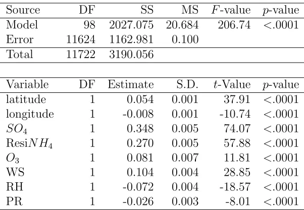
4.1 Spearman Rank Correlation Coefficients between Variables . . . 74 4.2 ANOVA Table for LRM . . . 80 4.3 Mean and S.D. of Posterior Medians of Significant Regression
Coeffi-cients for SO4 . . . 85
4.4 Mean and S.D. of Posterior Medians of Significant Regression Coeffi-cients for ResidualN H4 . . . 86
4.5 Mean and S.D. of Posterior Medians of Significant Regression Coeffi-cients for O3 . . . 88
4.6 Mean and S.D. of Posterior Medians of Significant Regression Coeffi-cients for Wind Speed . . . 90 4.7 Mean and S.D. of Posterior Medians of Significant Regression
Coeffi-cients for Relative Humidity . . . 92 4.8 Mean and S.D. of Posterior Medians of Significant Regression
List of Figures
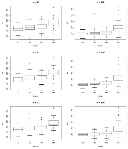
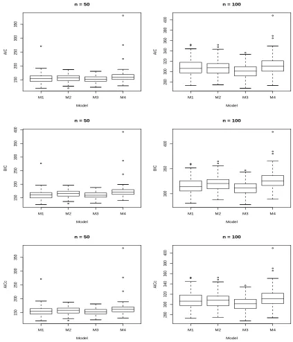
3.1 Box Plots for Each Criterion Obtained by Fitting Each Model to D1 . 50
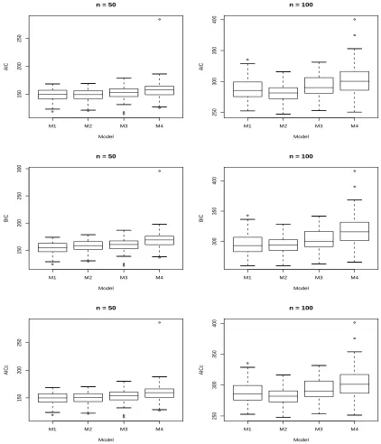
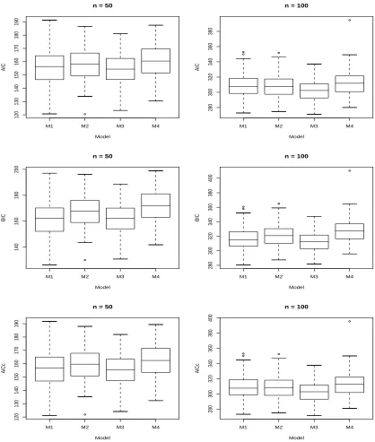
3.2 Box Plots for Each Criterion Obtained by Fitting Each Model to D21 53
3.3 Box Plots for Each Criterion Obtained by Fitting Each Model to D22 54
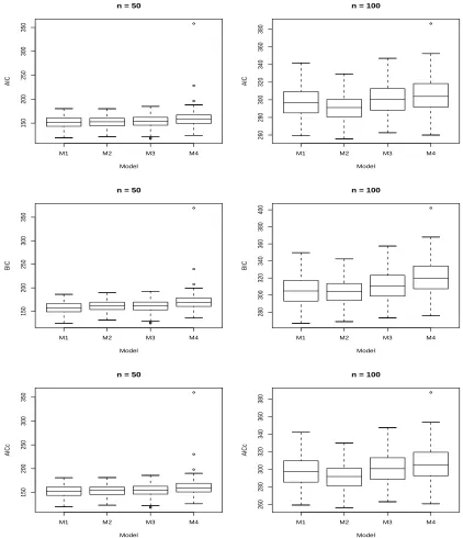
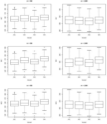
3.4 Box Plots for Each Criterion Obtained by Fitting Each Model to D31 57
3.5 Box Plots for Each Criterion Obtained by Fitting Each Model to D32 58
3.6 Box Plots for Each Criterion Obtained by Fitting Each Model to D41 61
3.7 Box Plots for Each Criterion Obtained by Fitting Each Model to D42 62
3.8 Box Plots for Each Criterion Obtained by Fitting Each Model to D43 63
3.9 Box Plots for Each Criterion Obtained by Fitting Each Model to D44 64
4.1 Locations of Stations . . . 69
4.2 Histogram for T N O3 and log(T N O3) . . . 77
4.3 Space-Time Correlogram for the Residual of LRM . . . 81
4.4 Frequencies and Box Plots for Posterior Medians of Significant Weeks in Each Month forSO4 . . . 84
4.5 Frequencies and Box Plots for Posterior Medians of Significant Weeks in Each Month for Residual N H4 . . . 86
4.6 Frequencies and Box Plots for Posterior Medians of Significant Weeks in Each Month forO3 . . . 87
4.7 Frequencies and Box Plots for Posterior Medians of Significant Weeks in Each Month for Wind Speed . . . 89
4.8 Frequencies and Box Plots for Posterior Medians of Significant Weeks in Each Month for Relative Humidity . . . 91
4.9 Frequencies and Box Plots for Posterior Medians of Significant Weeks in Each Month for Precipitation . . . 93
4.10 Spatial Correlogram and Fitted Exponential Correlation Model . . . 96
A.1 Box Plots for HN O3 by Siteid, Year and Month . . . 107
A.2 Box Plots for N O3 by Siteid, Year and Month . . . 108
A.3 Box Plots for T N O3 by Siteid, Year and Month . . . 109
A.5 Box Plots for N H4 by Siteid, Year and Month . . . 111
A.6 Box Plots for O3 by Siteid, Year and Month . . . 112
A.7 Box Plots for Temperature by Siteid, Year and Month . . . 113
A.8 Box Plots for Dew Point Temperature by Siteid, Year and Month . . 114
A.9 Box Plots for Solar Radiation by Siteid, Year and Month . . . 115
A.10 Box Plots for Wind Speed by Siteid, Year and Month . . . 116
A.11 Box Plots for Relative Humidity by Siteid, Year and Month . . . 117
Chapter 1
Introduction
Researchers in diverse areas such as environmental and health sciences are increas-ingly faced with working with data that are observed over space and time. These data arise because of advances in data collection methods, which use state of the art equipment for collecting data from such platforms as radars and satellites. Increased computational resources aid in the analysis of these data. The use of space-time data can be found in many applications. For example, we investigate a set of space-time data that involves the analysis of nitrate concentrations and their relations to mete-orological data such as temperature, relative humidity, wind speed and precipitation and chemical data such as sulfate, ammonium, and ozone as predictors. This data set was collected at selected monitoring sites on a weekly basis over several years in the eastern part of United States. We describe some general features of this spa-tial/temporal data set in Chapter 4.
mechanisms of data collection procedures. Let D ⊆ Rd(d ≥ 2) denote a domain in the space where we collect data and s ∈ D represent the location of a site. Point referenced dataare often referred to as geostatistical data and typically arise when the spatial locationsvaries continuously over a fixed study regionD. For example, in our application to an air pollution problem, data are collected over a domain in the eastern U.S. The data are called arealorlattice datawhere the fixed domain Dis partitioned into a finite number of areal units with well defined boundaries such as postal codes or counties. Here an observation is thought to be associated with an areal unit of non-zero volume as opposed to a particular location point. Spatial point pattern data arise when an event of interest (e.g., an outbreak of a disease) occurs at random locations. In this case, the domain D is random and its index set gives the spatial point pattern. In some cases this information might be supplemented by additional covariate information at the event locations. See Chapter 1 of Schabenberger and Gotway (2005) for additional discussion on spatial data types.
Similar to spatial data, time series data can be categorized into continuous or discrete. Continuous time series data are observed at every instant of time (e.g., lie detectors), and discrete time series data are usually observed at regularly spaced intervals (e.g., weekly share prices and daily rainfall). Notice that frequently observed discrete time series data can be used to approximate a continuous time series.
1.1
Statistical Models for Space-Time Data
In recent years, there has been widespread attention in the statistical literature given to models for space-time data (Mardia et al., 1998; Kyriakidis and Journel, 1999; Wikle and Cressie, 1999; Stroud et al., 2001; Gelfand et al., 2005). Often, in modeling space-time data, it is of interest to predict the time evolution of a response variable over a given spatial domain. To this end, statistical models are employed to obtain accurate predictions of a response variable, such as nitrate concentrations.
Following Banerjee et al. (Chapter8, 2004), the general form of models for space-time data can be defined as
Z(si, t) =Y(si, t) +ǫ(si, t), i= 1,· · · , n, t= 1,· · · , m, (1.1)
where Z(si, t) represents the observed response variable, Y(si, t) represents the
un-derlying space-time process andǫ(si, t) represents the error process which is assumed
to be a white noise process. The space-time process Y(si, t) can be expressed as
Y(si, t) =µ(si, t) +ω(si, t), (1.2)
where µ(si, t) is a mean process and ω(si, t) is a zero mean space-time process. We
generally assume theǫ-process to be independent of theω-process. The mean process is usually modeled using parametric or nonparametric regression with a set of observed covariates x(si, t). A parametric covariance structure is typically assumed for the
ω(si, t) process. The space-time covariance function is defined as
The space-time process ω(s, t) is said to be stationary if
C(s1, s2;t1, t2) = C(s1 −s2;t1−t2) = C(d;τ), (1.4)
where d = s1 −s2 and τ = t1−t2 denote the separation vectors, which means the
space-time covariance function is a function of the separation vectors. A stationary process is said to beisotropic if
C(d;τ) =C(||d||;|τ|), (1.5)
that is, the covariance function depends on the separation vectors only through their lengths ||d|| and |τ|. Processes which are not isotropic are called anisotropic. In the literature isotropic processes are popular because of their simplicity and interpretabil-ity. An isotropic process ω(s, t) is said to be separable if
C(||d||;|τ|) = Cs(||d||)Ct(|τ|). (1.6)
Suitable forms for the functions Cs(·) and Ct(·) are available in the literature. A
popular choice for Cs(·) is the Matern covariance (Matern, 1986) function and the
ARMA (Box and Jenkins, 1976) covariance function forCt(·).
Space-time models are often constructed by combining traditional time series tech-niques with methods from spatial statistics. In the time series context, popular ap-proaches include ARIMA models (Box, Jenkins and Reinsel, 1994) for stationary data, and dynamic linear models (West and Harrison, 1997), which allow for nonstationary components such as temporal trends and seasonality.
Early attempts to develop space-time models assumed temporal stationarity. In an early Bayesian application, Handcock and Wallis (1994) considered the space-time modeling of winter temperature data observed over a region in the northern United States. They employed stationary Gaussian process models with an AR(1) model for the time series at each location and carried out separate spatial analyses to study global warming in each year. Carroll et al. (1997) again used stationary Gaussian processes, assuming a separable form for the space-time covariance function to study ground level ozone. Their model combines trend terms incorporating temperature and hourly or monthly effects, and an error model in which the correlation in the residuals is a nonlinear function of time and space, in particular the spatial structure is a function of the lag between observations. Brown et al. (2000) considered the space-time modeling of rainfall data using a non-separable model. They showed that this model is well suited to a wide range of realistic problems which will be poorly fitted by separable models.
func-tion of time of day. Other approaches involving hierarchical Bayesian models include Wikle et al. (1999) and Waller et al. (1997). Wikle et al. (1999) analyzed monthly maximum atmospheric temperatures and Waller et al. (1997) used generalized linear models to map lung cancer rates in Ohio.
There is also much recent space-time modeling, which employs a Markov random field structure in the form of conditionally autoregressive (CAR) specifications. Waller et al. (1997) studied disease mapping, and Gelfand et al. (1998) looked at single family home sales. Pace et al. (2000) worked with simultaneous autoregressive (SAR) models extending them to allow temporal neighbors as well as spatial neighbors.
a lattice framework and the updates have a relatively low computational load using the Kalman filtering and smoothing algorithms. Kriging is a common interpolation technique used for making spatial predictions at locations where measurements have not been obtained. Points which are close together have a higher spatial correlation than points that are far apart. Predictions at unmeasured locations are based on a weighted average of measured locations, where weights are assigned to all points based on the rate of information decay when moving away from a measurement point. Sans´o and Guenni (1999) proposed a DLM with unknown covariance parameters to model rainfall data. Tonellato (1997) developed a state-space model with both stationary and nonstationary temporal components, which was applied in Tonellato (1998) to an Irish wind power prediction problem. Huerta et al. (2004) modeled ozone concentrations over Mexico City and carried out spatial as well as temporal interpolation and prediction using DLM. Banerjee et al. (2005) discussed univariate space-time dynamic models and multivariate spatial dynamic models. They allowed for nonlinear mean structure and non-stationary association structure in modeling space-time data.
State-space approaches in a non-Bayesian setting include Huang and Cressie (1996) and Mardia et al. (1998). Huang and Cressie (1996) modeled snow water in time and space using a separable dynamic model. Mardia et al. (1998) proposed a kriged Kalman filter and outlined a likelihood-based estimation strategy.
complex-ity. Also, the dimension of space-time data sets can be very large, and moreover, space-time processes are often complicated in that the dependence structure across space and time is non-trivial, often non-separable and non-stationary in space and/or time. Hence, space-time modeling is a challenging task which requires the manipula-tion of large data sets and the ability to fit realistic and complex models. In particular, parameter estimation can be problematic due to the high dimensionality. Parameter identifiability is often a difficult task with high dimensional models. Several modeling strategies have been proposed to address this problem. Many authors have consid-ered ways of reducing the computational load of the multivariate DLM. A common approach is to reduce the number of dimensions, for instance by constructing the update using summary variables. Wikle and Cressie (1999) developed a space-time Kalman-filter that achieves dimension reduction by decomposing the state-process into sets of basis functions and time series. To avoid a high computational load they used an empirical Bayesian method for the estimation of model parameters rather than a fully Bayesian hierarchical approach. However, the additional variability in estimating parameters is ignored in such a method. Stroud et al. (2001) specified very simple random walk dynamics, while Xu and Wikle (2004) discussed efficient estima-tion approaches via the expectaestima-tion-maximizaestima-tion (EM) algorithm for the parameter and covariance matrices with high dimensionality in dynamic space-time models.
to be used for a covariance function within dynamic space-time modeling framework. Using this unconstrained reparametrization method, we are able to implement the models to fit high-dimensional data without many restrictive assumptions. We take a Bayesian approach and use Markov chain Monte Carlo (MCMC) simulation tech-niques to obtain the parameter estimates followed by predictive inference. Recent developments in MCMC computing allow fully Bayesian analyses of complex multi-level models for dynamic space-time data. Pole et al. (1994) and West and Harrison (1997) are good references on the dynamic models from a Bayesian point of view.
1.2
Model Selection Methods
Model choice is a crucial issue in statistical data analysis. Researchers typically consider a number of plausible models in statistical applications, and hence model comparison is required to identify the “best ” model among several candidate models. Model comparison enables the selection of a suitable model based on a given data set and other modeling information. A variety of model selection methods are available in the literature. We discuss these methods in this section.
Hypothesis testing is probably the most frequently used method in model selection. In particular, sequential hypothesis testing has most often been used. Sequential testing can be performed via one of the forward, backward, and stepwise methods. The forward method begins with no variables in the model. Then variables are added one by one to the model until no remaining variable produces a significant F
statistic calculated for each variable reflects the variable’s contribution to the model if it is included. The backward method begins with all of the variables included in the model. Then the variables are deleted from the model one by one until all the variables remaining in the model produce significant F statistics. At each step, the variable showing the smallest contribution to the model is deleted. The stepwise method modifies the forward and backward methods and differs in that variables can be added or deleted at each step. This stepwise process ends when none of the variables outside the model has a significant F statistic and every variable in the model is significant.
However, hypothesis testing is defined only for nested models. A model M1 is
called nested under M2 if M1 is a special case of model M2. Also, Akaike (1974)
stated that hypothesis testing, in general, performs very poorly when used for model selection.
Cross-validation is one of the methods that also has been suggested for model selection (Stone, 1974). The holdout method is the simplest kind of cross validation. The data set is separated into two sets, called the training set and the testing set. The training set is used for model fitting, and the testing set is used for model validation. One predicts the data in the testing set using the fitted model based on the training set. Then a best model is selected by a chosen criterion such as minimum squared prediction error. However, this method depends heavily on how the division is made.
are put together to form a training set. Then the average error across all k trials is computed. The advantage of this method is that it matters less how the data gets divided, however it becomes computationally very intensive. A variant of this method is to randomly divide the data into a test and training set k different times. The advantage of doing this is that one can independently choose how large each test set is and how many trials you average over.
The adjusted coefficient of multiple determination (R2) has been used in model
selection for classical multiple linear regression analysis. This is computed as
1−(1−R2)
n−1
n−p
,
whereR2 is the usual coefficient of multiple determination (Draper and Smith, 1981).
Under this method, one selects the model in which this adjusted statistic is largest. McQuarrie and Tsai (1998) found this approach to be very poor in model selection.
Mallows’ Cp (Mallows 1973) statistic is well known for variable selection, but
limited to multiple linear regression problems with normal errors. Mallows’ Cp is
computed as
Cp =
SSres
M Sres
−n+ 2p,
where SSres is the residual sum of squares for the model with p−1 variables, M Sres
is the residual mean square when using all available variables, n is the number of observations, andpis the number of variables used for the model plus one. The general procedure to find an adequate model by means of the Cp statistic is to calculate Cp
for all possible combinations of variables. The model with the lowest Cp value which
Information criteria have played an important role in model selection. These criteria are based on information theory. The basis for the information-theoretic approach to model selection is the Kullback-Leibler (K-L) information (Kullback and Leibler, 1951) given by,
I(f, g) =
Z
f(x)log
f(x)
g(x|θ)
dx,
where θ represents parameters in model g. Here, I(f, g) can be interpreted as the “information lost when the model g is used to approximate full reality or truth f” (Burnham and Anderson, Section 2.1, 2002). I(f, g) also can be interpreted as a “distance ” from the approximating modelg to truth f. We seek to find a candidate model that minimizes I(f, g) over the candidate models. However, I(f, g) cannot be used directly because it requires knowledge of f(x) and the parameters in models
g(x|θ).
Akaike’s information-theoretic approach has led to a number of methods having desirable properties for the selection of the best approximating models in practice. Akaike (1973) provided a way to estimate relative, expected I(f, g) based on the empirical log-likelihood function. He found that the maximized log-likelihood value was a biased estimate of the relative, expected K-L information, and that under certain conditions this bias was approximately equal to p, the number of parameters in the approximating model g. His method, Akaike’s Information Criterion (AIC) is based on this finding. AIC is defined as,
AIC =−2loghL(ˆθ|X)i+ 2p,
denotes the number of paramters in the model.
Takeuchi (1976) derived a general method to get from K-L information to AIC. He derived an asymptotically unbiased estimator of the relative, expected K-L in-formation without special conditions. Takeuchi’s Inin-formation Criterion (TIC) has a more general bias adjustment term,
TIC = −2loghL(ˆθ|X)i+ 2tr J(θ)I(θ)−1
,
whereJ(θ) represents the variance matrix of the first-order derivatives,I(θ) represents minus the expected value of the matrix of second-order derivatives of the log-likelihood with respect to the parameter θ and “tr ” denotes the matrix trace function. AIC is an approximation to TIC, where tr(J(θ)I(θ)−1) =p. TIC requires large sample sizes
to estimate the elements of the twop×p matrices in the bias-adjustment term. This criterion is known to be useful when the candidate models are not particularly close approximations tof (Burnham and Anderson, 2002).
The method for small sample approximations, called Corrected AIC (AICc), was proposed by Sugiura (1978) and Hurvich and Tsai (1989). They pointed out that AIC may perform poorly if the number of parameters are too large in relation to the size of the sample. AICc is defined as,
AICc =−2loghL(ˆθ|X)i+ 2p
n
n−p−1
,
where n is sample size. Unless the sample size is large with respect to the number of estimated parameters, use of AICc is recommended.
easy to compute and quite effective in many applications. In most practical situations, AIC and AICc are very useful approximations to the relative K-L information.
QAIC and QAICc, based on quasi-likelihood theory, have been derived for appro-priate model selection when count data are found to be overdispersed. If overdisper-sion is found in the analysis of count data, the nominal log-likelihood function must be divided by an estimate of the overdispersion to obtain the correct log-likelihood. The principles of quasi-likelihood suggest simple modifications to AIC and AICc (Lebreton et al., 1992). QAIC and QAICc are defined as,
QAIC = −2loghL(ˆθ|X)/ˆci+ 2p,
QAICc = −2loghL(ˆθ|X)/ˆci+ 2p
n
n−p−1
,
where ˆcis an estimated overdispersion factor.
AIC, AICc, QAIC, and QAICc are estimates of the relative K-L distance between truthf and the approximating modelg. These criteria were motivated by the concept that the truth is very complex and that no true model exists. Thus, one could only approximate truth with a model, say g. Given a good set of candidate models for the data, one could estimate which approximating model is best. TIC allows that the set of candidate models does not include f or any model similar to f (Burnham and Anderson, 2002).
selecting this true model approaches one as sample size increases. The best known of these dimension-consistent criteria is the Bayesian Information Criterion (BIC), which was derived by Schwarz(1978) in a Bayesian context. It is defined as,
BIC =−2loghL(ˆθ|X)i+plog(n),
wherepis the dimension of the model andnis sample size. BIC arises from a Bayesian viewpoint with equal prior probability on each model and very vague priors on the parameters, given the model. BIC is not an estimator of relative K-L information. Bozdogan (1987) provides a review of many of the other dimension-consistent criteria.
Spiegelhalter et al. (2002) have developed a Deviance Information Criterion (DIC) from a Bayesian perspective that is analogous to AIC. DIC is one of the common methods for model comparison in the Bayesian framework. It is defined as,
DIC =−2log
L(¯θ|X)
+ 2pDIC,
where ¯θ =E[θ|X] denotes the posterior mean ofθgiven the dataX, andpDIC denotes
the effective number of parameters given by pDIC =E[D(θ)|X]−D(E[θ|X]), where
D(θ) =−2log[L(θ|X)] denotes the deviance of the model. DIC seems to behave like AIC rather than like BIC (Spiegelhalter et al., 2002). One disadvantage of DIC is that it usually requires computationally intensive methods like Markov Chain Monte Carlo (MCMC) approach to compute both of its components.
while still being loyal to the original data. A simplified version of this predictive cri-terion computes the predictive mean of the squared difference between the observed data and a replicate of data under the model, and chooses the model with the small-est value. The predictive criterion can also be decomposed into two terms (Gelfand and Ghosh, 1998). The first term can be viewed as a goodness of fit term with the mean of the posterior predictive distribution of the replicate replacing the maximum likelihood estimate of the mean, and the second term is a variance term that can be thought of as a penalty function. Gelfand et al. (1998) adopt this criterion to select a model for the analysis of residential sales data based on a variety of space-time models.
The principle of parsimony provides a basis for model selection. As the goal of model selection using information criteria is to select parsimonious models, models that minimize the criterion are selected.
Chapter 2
A Reparametrization Approach for
Dynamic Space-Time Models
2.1
Introduction
Statistical modeling of time series processes is usually based on classes of dynamic models. The term dynamic relates to changes in such processes due to the passage of time. Following West and Harrison (1997), in a Bayesian framework, forecasting problems through dynamic modeling are structured using four fundamental principles:
(i) sequential model definition,
(ii) structuring using parametric models,
(iii) probabilistic representation of information about parameters, and
Suppose that the time origin, t = 0, represents the current time, and that the existing information available is denoted by D0, the initial information set. This
represents all the available relevant starting information which is used to form ones initial views about the future. In forecasting ahead to any time t1 >0, the primary
objective is calculation of the forecast distribution for (Yt1|D0), where Yt1 is the ob-servation at time t1. Generally, we denote by Dt the information set available at
time t. Thus statements made at time t about any random quantities of interest are based on Dt. In particular, forecasting ahead to time t2 > t1 involves consideration
of the forecast distribution for (Yt2|Dt1). Observing the value of Yt2 at time t2 im-plies that Dt2 includes both the previous information set Dt1 and the observation
Yt2, that is, Dt2 ={Yt2, Dt1}, which represents information updating. The sequential focus is emphasized through the use of statistical models for the development of the series into the future described via distributions for Yt2, Yt3(t3 > t2),· · ·, conditional on past information Dt1. From now on we assume that the temporal observations are collected at regular time interval denoted by t = 1,2,· · ·. Focusing on one-step ahead, the forecaster’s views are then structured in terms of a parametric model,
p(Yt|θt, Dt−1),
whereθtrepresents the parameter vector at timet. Indexingθtbytindicates that the
parameterization is dynamic. The model parameter θt provides the means by which
information relevant to forecasting the future is summarized and used in forming forecast distributions. The learning process involves sequentially revising the state of knowledge about such parameters. At time t, historical information Dt−1 is
p(θt|Dt−1) and the posterior densityp(θt|Dt) provide a concise, coherent and effective
transfer of information on the time series process through time. An ultimate goal is attained by directly applying probability laws. That is,
p(Yt,θt|Dt−1) = p(Yt|θt, Dt−1)p(θt|Dt−1),
from which the relevant one-step forecast may be deduced as the marginal
p(Yt|Dt−1) =
Z
p(Yt,θt|Dt−1)dθt.
Inference for the future Yt is now a standard statistical problem of summarizing the
information encoded in the forecast distribution.
2.2
Dynamic Linear Models
Let yt be a n ×1 vector of observations at time t. yt is modeled conditionally based on ap×1 vector, θt, called the state vector, through a measurement equation or a observation equation. In general, the elements of θt are not observable, but are generated by a first-order Markovian process, resulting in a transition equation or evolution equation. Therefore, we can describe the above framework for t= 1,2,· · ·, as
Observation equation : yt =Ftθt+υt, υt ∼N(0,Συt),
Evolution equation : θt=Gtθt−1+ηt, ηt∼N(0,Σ η t),
where Ft and Gt are n ×p and p×p matrices, respectively. The first equation is
the observation equation, where υtis an×1 vector of serially uncorrelated Gaussian
variables with mean zero and an×n covariance matrix, Συ
t. The second equation is
the evolution equation withηt being ap×1 vector of serially uncorrelated zero-mean Gaussian disturbances and Σηt the correspondingp×pcovariance matrix. The model is completed with a Gaussian prior on the initial state: θ0 ∼ N(m0, C0), with θ0
independent of υt and ηt. We further assume thatηt and υt are independent.
Ft and Gt are referred to as system matrices which are allowed to change over
time. The matrix Ft is usually specified by the design of the problem at hand, while
Gtis specified through modeling assumptions; for example,Gt =Ip, thep×pidentity
matrix would render a vector autoregressive (VAR) random walk of order oneV AR(1) process for θt. A random walk prior is a natural choice when no prior information
The evolution variance matrix Σηt can be specified either explicitly or through a
dis-count factorδ∈(0,1], which defines Σηt = 1−δδPt, withPt =V ar(Gtθt−1|y1,· · · ,yt−1).
When p is large, the discount method is usually preferred, since it requires elicita-tion of only one parameter instead of p(p+ 1)/2. The observation variance matrix Συ
t is usually assumed to be a diagonal matrix. We will show that our proposed
reparametrization method allows one to relax these restrictive assumptions.
2.3
Dynamic Space-Time Models (DSTM)
We adapt the above DLM framework to space-time data. The approach taken here is to view the data as arising from a time series of spatial processes.
Suppose the process Z(s, t) is observed on a finite number of sites labeled as
s1, ..., sn at each time t, wheret = 1,2,· · ·, m. Consider the n×1 vector time series
Zt = (Z(s1, t), ..., Z(sn, t))T at time t. For each t, the DLM is usually formed by an
observation equation and an evolution equation. An observation equation describes the relationship between the observation (Zt) and the regressors (Xt) that takes the
form of a multivariate regression process,
Zt=Xtβt+νt, νt∼N(0,Σνt) (2.1)
where Xt is an n×p observed design matrix and βt is a p×1 vector of regression
coefficients or state parameters. An evolution equation describes the dynamics of the vector of regression coefficients or state parameters βt through time,
where Gt is a p×p evolution matrix. There are several ways to model the Gt’s.
The most common assumption is that the Gt’s are structurally known, possibly up
to some finite number of parameters. In this thesis, we do not make any structural assumption about the Gt’s but we assume thatGt=Gfor all t and that G follows a
matrix-valued normal distribution with meanG0 and variance-covariance parameters
Ω0 and ΣG0. That is, G∼ M Np×p(G0, Ω0,ΣG0). We also assume that the νt and ωt
error vectors are independent and have multivariate normal distributions with mean 0 and variance-covariance matrices Σν
t and Σωt, respectively. The model is completed
with a normal prior for the initial state, β1 ∼N(β0,Σω
0), where β0 is known.
Equivalently, the model can be written using hierarchical specifications as follows:
Zt|βt ∼ N(Xtβt,Σνt),
βt|βt−1, G ∼ N(Gβt−1,Σωt),
G ∼ M N(G0,Ω0,ΣG0),
β1 ∼ N(β0,Σω0),
where the matrix valued normal distribution M N(G0,Ω0,ΣG0) has the probability
density function given by
p(G|G0,Ω0,ΣG0) = (2π) −p2
/2|Ω0|−p/2|ΣG
0|
−p/2exp
−1
2tr
h
Ω0−1(G−G0)ΣG0 −1
(G−G0)T
i
.
This Bayesian hierarchical approach not only helps organize our thinking about the model, but also fully accounts for all sources of uncertainty without making substan-tial structural assumptions like, spasubstan-tial stationarity, isotropy, etc.
In order to keep our illustrations simple, first we consider the following simplified DLM. Specifically, we assume that Σν
That is, variance-covariance matrices Σν and Σω do not change over time (and hence
are static). Our simplified DLM can be written as,
Zt = Xtβt+νt, νt ∼N(0,Σν), (2.3)
βt = Gβt−1+ωt, ωt∼N(0,Σω), (2.4)
andβ1 ∼N(β0,Σω
0). Here, Σν and Σω are unstructured variance-covariance matrices
and for the ease of exposition, we initially assume that Zt and Xt are observed at
all time points t. Later we discuss how to relax this assumption if some observations are missing.
The Bayesian model is completed with the specification of a prior distribution for the parameters. These include the data-model covariance matrix Σν and the error
covariance matrix Σω. Prior specifications for Σν and Σω can be tricky as these
matrices are usually high-dimensional (e.g., Σν isn×n) and they need to be positive
definite (pd). It is customary to use the inverse Wishart distributions to model such covariance matrices. Note that our models require no restrictive assumptions such as stationarity and isotropy as Σν is left unstructured. However, if such assumptions
are deemed necessary, we can easily incorporate them in our modeling framework.
As we mentioned earlier, inference for dynamic models is made sequentially by obtaining the prior predictive and updated distributions for the state parameters βt
for each time t. The prior predictive distributions are respectively obtained by
p(βt|Dt−1) =
Z
p(βt|βt−1)p(βt−1|Dt−1)dβt−1
p(Zt|Dt−1) =
Z
and the updated distribution is obtained by Bayes’ theorem as
p(βt|Dt)∝p(Zt|βt)p(βt|Dt−1)
where Dt represents all the available information upto time t.
2.4
Model Fitting
The most popular computing tools in Bayesian practice today are Markov chain Monte Carlo (MCMC) methods. This is due to their ability to enable inference from posterior distributions of arbitrarily large dimension, essentially by reducing the problem to one of recursively solving a series of lower-dimensional problems. Like traditional Monte Carlo methods, MCMC methods work by producing not a closed form for the posterior, but a sample of values {θ(l), l = 1,· · · , B} from this
distrib-ution. While this obviously does not carry as much information as the closed form itself, a histogram or kernel density estimate based on such a sample is typically suf-ficient for reliable inference. Moreover such an estimate can be made accurate merely by increasing the Monte Carlo sample size B. However, unlike traditional Monte Carlo methods, MCMC algorithms produce correlated samples from the posterior, since they arise from recursive draws from the path of a Markov chain, the stationary distribution of which is the same as the posterior.
Suppose our model features p parameters, θ = (θ1,· · ·, θp)T. To implement the
Gibbs sampler, we must assume that samples can be generated from each of the full conditional distributions {p(θi|θj6=i,y), i = 1,· · · , p} in the model, where y denotes
distributions uniquely determine the joint posterior distribution, p(θ|y), and hence all marginal posterior distributions p(θi|y), i = 1,· · · , p. Given an arbitrary set of
starting values {θ(0)2 ,· · · , θp(0)}, the algorithm for the Gibbs sampler proceeds as
fol-lows:
Step 1Draw θ(1l) fromp(θ1|θ2(l−1), θ3(l−1),· · ·, θ(pl−1),y)
Step 2Draw θ(2l) fromp(θ2|θ1(l), θ3(l−1),· · · , θp(l−1),y)
...
Step p Draw θ(pl) fromp(θp|θ1(l), θ (l)
2 ,· · · , θ (l)
p−1,y)
The cycles from Step 1 to Step p are repeated for l = 1,· · · , B. Under mild regu-latory conditions that are generally satisfied for most statistical models (see Geman and Geman, 1984), one can show that {θ1(l),· · · , θp(l)} converges in distribution to a
draw from the true joint posterior distributionp(θ1,· · · , θp|y). This means that forl
sufficiently large, say l0,{θ(l), l =l0+ 1,· · · , B} is a sample from the true posterior,
from which any posterior quantities of interest may be estimated. For example, a histogram of the {θ(il), l = l0 + 1,· · · , B} provides a simulation-consistent estimator
of the marginal posterior distribution forθi, p(θi|y). The time froml = 0 tol =l0 is
commonly known as the burn-in period, and posterior estimates are obtained using
{θ(l), l =l0+ 1,· · · , B}.
We fit our model using a Markov chain Monte Carlo (MCMC) procedure known as the Gibbs sampler (Geman and Geman, 1984; Gelfand and Smith, 1990) via the
WinBUGS software which is a window-based software package for Bayesian analysis using MCMC methods. The software can be downloaded from the website
The updating scheme in the dynamic space-time model may not be easy to imple-ment when theGmatrix is completely unknown. Further these types of multivariate updating schemes can be very unstable and time consuming when the dimensions are very large. In order to avoid such numerical instabilities and to accelerate model fit-ting, we describe an equivalent univariate scheme for the aforementioned DLM using a reparametrization method in the next section. As by-products of this reparame-trization method, we obtain several extensions of the usual DLM.
2.5
A Reparametrization Method
type of reparameterization of covariance matrices has been used only to model tem-poral processes, taking advantage of the natural ordering of time. We extend these methodologies to spatial and temporal processes and show several extensions.
For our DLM framework, we define two lower triangular matrices Tν and Tω
and two diagonal matrices Dν and Dω such that TνΣνTν T = Dν and TωΣωTωT =
Dω. Such decompositions of positive definite matrices are unique. More precisely,
let Tν and Tω be the lower triangular matrices with 1’s as their diagonal entries
and −φii′, i > i′ and −ψkk′, k > k′ as their lower triangular entries, respectively.
Also, letDν andDω be diagonal matrices with entriesσν
12,· · · , σnν2 andσ1ω2,· · ·, σpω2,
respectively. We now re-express the equations (2.3) and (2.4) using the entries of their lower triangular and diagonal matrices.
Let Zit = Z(si, t), i = 1,· · · , n, t= 1,· · · , m and Xitk = Xk(si, t), k = 1,· · ·, p.
Notice that Zt = (Z1t,· · · , Znt)T and {Xt}n×p = ((Xitk))1≤i≤n,1≤k≤p, which appear
in (2.3). Then we can represent the DLM defined by (2.3) and (2.4) as follows. The observation equation can be written as,
Zit =
p
X
k=1
βktXitk+
i−1
X
i′=1
φii′Zi′t+νit, (2.5)
Z1t =
p
X
k=1
βktX1tk+ν1t, (2.6)
where i = 2,· · · , n, t = 1,· · · , m, E[νit] = 0, E[νit2] = σνi2, and E[νitνi′t] = 0, i 6= i′.
written as,
βkt =
p
X
k′=1
βk′t−1gkk′+
k−1
X
k′=1
ψkk′βk′t+ωkt, (2.7)
β1t =
p
X
k′=1
βk′t−1g1k′ +ω1t, (2.8)
where k = 2,· · · , p, t = 2,· · · , m, E[ωkt] = 0, E[ω2kt] = σkω2, and E[ωktωk′t] = 0,
k 6=k′, and initial state equation can be written as,
βk1 =βk0+
k−1
X
k′=1
ψkk′βk′1+ωk1, (2.9)
where k = 2,· · · , p. Notice that ωt = (ω1t,· · · , ωnt)T as in (2.2). The model is
completed with
β11 =β10+ω11.
Here, notice that no structural constraints are required for the elements ofTν,Tω,Dν,
and Dω (i.e., φ
ii′, ψkk′ ∈R and σiν2, σkω2 ∈(0,∞)). In particular, for our applications
we may specify a prior distribution for these parameters as,
φii′ ∼ N(φ0, σφ2), 1≤i′ < i≤n,
ψkk′ ∼ N(ψ0, σψ2), 1≤k′ < k ≤p,
σ2
νi ∼ IG(aν, bν), i= 1,· · · , n,
σ2ωk ∼ IG(aω, bω), k= 1,· · · , p,
gkk′ ∼ N(g0, σ2g), k, k′ ∈1,· · · , p,
where φ0, σφ2, ψ0, σ2ψ, aν, bν, aω, bω, g0 and σg2 are all known values that can be used
generate a set of vague priors. Here N(a, b) denotes a normal distribution with mean
a and varianceb, andIG(a, b) denotes an inverse gamma distribution with mean a−b1
for a > 1 and variance b2
(a−1)2(a−2) for a > 2. For instance, we choose these values
in such a way that these will have minimal impact on the posterior inference of the parameters. Other prior distributions can also be adapted for our framework very easily.
Using this reparametrized univariate scheme we can avoid numerical instabilities due to high dimensionality. The routine handling of missing data is also apparent by using the reparametrization scheme. If an observation is missing, we just sample it from its full conditional distribution. We illustrate the use of this reparametrization method by applying our model to a set of nitrate concentration data in Chapter 4.
The advantages of our proposed reparametrized dynamic space-time models (RD-STM) can be summarized as follows:
i) Numerical stability: RDSTM avoids numerical instabilities caused by multivari-ate updating scheme when the dimensions are very large.
ii) Routine handling of missing data: RDSTM allows missing data to be imputed from its full conditional distribution.
iii) Implementation using WinBUGS: RDSTM can be implemented using Win-BUGS, while multivariate scheme of DSTM cannot.
are as follows:
i) Dynamic modeling of covariance function Σν and Σω: we can allow Σν and Σω
to depend on t, that is, φii′’s, ψkk′’s, σνi2’s, and σkω2’s depend on t and thus
making these parameters dynamic as well.
ii) Relaxing the Gaussian assumption of distributions for νt’s and ωt’s: we can
assume other than Gaussian distributions such as t-distributions for νt’s and
ωt’s.
iii) Extension of the first-order Markovian assumption: we can assumeθt is gener-ated by a higher order Markovian process rather than a first-order in evolution equations in (2.7) and (2.8).
There are several space-time models available in the literature and it is almost impossible to compare our proposed model to all such models. But we provide a brief description of a model that closely resembles ours and we compare our models to that proposed by Wikle and Cressie (1999).
2.6
Comparison with Space-Time Kalman Filter
dimension reduction. The model is of the form,
Zt = yt+υt, υt ∼N(0, R),
yt = Φat+νt, νt ∼N(0, V),
at = Hat−1+Jηt, ηt∼N(0, Q),
where H = JB, J = (Φ′Φ)−1Φ′, and n×K matrices Φ and B are defined as Φ ≡
[φ(s1),· · · ,φ(sn)]′andB ≡[b(s1),· · · ,b(sn)]′. Here,φ(s)≡[φ1(s),· · ·, φK(s)]′,at≡
[a1(t),· · · , aK(t)]′, and b(s) ≡ [b1(s),· · · , bK(s)]′. {φj(s) : j = 1,· · · , K} are a
complete and orthonormal sequence of deterministic spatial functions, {aj(t) : t =
1,2,· · · .}is a random time series for eachj = 1,2,· · · , K, and{bj(s) :j = 1,· · · , K}
are unknown but nonstochastic parameters. Also,n denotes number of locations and
K denotes the key to dimension reduction.
Then the model can be written as,
Zt = Φat+υ∗t, υ
∗
t ∼N(0, R+V),
at = Hat−1+ηt∗, η∗t ∼N(0, JQJT).
That is, it has the same form as our dynamic space-time model (DSTM) except that Φ does not change over time and the variance matrices R+V and JQJT are also
assumed to be static over time.
Chapter 3
Performance of Information
Criteria for Spatial Models
there is no consensus on the best criterion for spatial model selection. Of particular interest is how these different criteria perform with various spatial covariance models. We explore this issue via Monte Carlo simulations in this chapter. The purpose of this study is to examine the performance of different information criteria for use in spatial covariance model selection. We compare the performance of traditional information criteria such as AIC, BIC, and Corrected AIC (AICc) (Sugiura, 1978; Hurvich and Tsai, 1989). This comparison is made using various spatial covariance models ranging from stationary isotropic to nonstationary models.
The remainder of this chapter is organized as follows. Section 3.1 introduces various information criteria used for model selection such as AIC, BIC and AICc. In Section 3.2, we describe various spatial covariance models such as stationary isotropic and anisotropic, and nonstationary models that will be used as an illustration to generate data from a specific covariance model. Finally, in Section 3.3., we present results from simulations which compare the performance of AIC, BIC and AICc with regard to their ability to identify the true model among various spatial covariance models.
3.1
Information-Theoretic Criteria for Model
Se-lection
for nested models, and this represents a limitation in the use of hypothesis testing in model selection.
Most information criteria have a form that consists of two terms. In general, the first term is the negative log-likelihood, multiplied by two, of the data calculated with the maximum likelihood estimates of the parameters; it represents the amount of information required to describe the data. The second term differs between different information criteria; it represents the amount of information required to describe the model. The second term can be interpreted as a penalty for model complexity; it thus increases as the number of parameters in the model increases. The basic principle of model selection using information criteria is to select statistical models that simplify the description of the data and model. Specifically, information methods emphasize minimizing the amount of information required to express the data and the model. This results in the selection of models that are the most parsimonious or efficient representations of observed data. To select parsimonious models, models minimizing information criteria are selected. In the following sections, we describe commonly used information criteria such as AIC, AICc, and BIC.
3.1.1
Akaike Information Criterion (AIC)
an estimate of KLD between a fitted model and the true model. AIC is defined as
AIC =−2loghL(ˆθ|X)i+ 2p, (3.1)
where logL(ˆθ|X) represents the log-likelihood function of the maximum likelihood estimator (MLE), ˆθ, given the observed data X, and p is the dimension of the para-meter θ. The first term can be interpreted as a measure of lack of model fit, while the second term can be interpreted as a penalty for increasing the dimension of the model. Recall that the second term is the asymptotic bias-correction term. It is the result of deriving an asymptotic estimator of relative expected KLD. In application, one computes AIC for each of the candidate models and selects the model with the smallest value of AIC. Models producing smaller values of AIC can be thought of as having a smaller difference from the true model, where the true model is unknown. AIC provides a simple and effective means for the selection of the best approximating model to the true model (Burnham and Anderson, 2002). With regard to general linear models, AIC is known to perform relatively well for small samples, however the criterion is large-sample inconsistent, which means AIC does not tend to select the true model in large samples (Hurvich and Tsai, 1990).
3.1.2
Corrected Akaike Information Criteria (
AICc
)
dimension of the model is large relative to sample size or whenn is small, for anyp. The AICc is defined as
AICc = −2loghL(ˆθ|X)i+ 2p
n
n−p−1
= −2loghL(ˆθ|X)i+ 2p+ 2p(p+ 1)
n−p−1 (3.2)
= AIC + 2p(p+ 1)
n−p−1,
where n is the sample size and p is the number of parameters in the model. AICc has an additional bias-correction term compared to AIC, which is adjusted to the parameter complexity p and the sample size n. However, if n is large with respect to p, then this additional bias-correction is negligible and AIC should perform well. Burnham and Anderson (2002) advocated the use of AICc, in particular, when the ratio n/p < 40 for the model with the largest value ofp. If n/p is sufficiently large, then AIC and AICc are similar and will tend to select the same model. They also mentioned that AICc should be used in practice, because AICc converges to AIC as n gets large, with pfixed.
3.1.3
Bayesian Information Criterion (BIC)
dimension-consistent criterion as we discussed in Section 1.2.4. BIC is defined as
BIC =−2loghL(ˆθ|X)i+plog(n), (3.3)
where loghL(ˆθ|X)i again represents the log-likelihood function of ˆθ, which is the maximum likelihood estimator (MLE) based on the observed dataX;pis the number of parameters in the model, and n is the sample size. The first term of BIC is same as that of AIC. However, the second term penalizes the model with increased model complexity, or larger p, and sample size as well. AIC and BIC differ only by the coefficient multiplying the number of parameters, in other words, by how strongly they penalize large models. In general, models chosen by BIC are more parsimonious than those chosen by AIC. As usually used, one computes the BIC for each model and selects the model with the smallest criterion value. In contrast to AIC, BIC is large sample model consistent, that is, BIC tends to choose the true model in large samples. However, BIC has also known to perform poorly in small samples in the context of general linear models (Hurvich and Tsai, 1990).
3.2
Spatial Models
3.2.1
Stationary Processes
Consider a random process {Z(s) : s ∈ D}, where D is a fixed subset of ℜd.
Assume that the random process Z(·) satisfies
E(Z(s)) =µ, for alls∈D and (3.4)
Cov(Z(si), Z(sj)) =C(si−sj), for allsi,sj ∈D. (3.5) That is, the mean does not depend on sand the covariance is a function only of the incrementsi−sj. ThenZ(·) is said to be a second-orderorweak stationary process.
Furthermore, ifC(si−sj) is a function ofksi−sjkonly, that is, the distance betweensi
andsj, thenC(·) is calledisotropic. An isotropic process assumes that the correlation structure between sites is circular which indicates the correlation depends only on the distance between sites.
One frequently used isotropic covariance function is the exponential model. Here the covariance between measurements at two locations is an exponential function of the distance between two locations,
Cov(Z(si), Z(sj)) =σ2exp(−φksi−sjk) +τ2I(i=j), σ2 >0, φ >0, τ2 >0, (3.6)
where ksi−sjk is the distance between sites si and sj, and I denotes the indicator
function. Hereσ2andφare positive parameters called the partial sill and the decay or
inverse range parameter, respectively. When i =j, dij = 0 and C(dij) =V ar(Z(si))
is often expanded to τ2+σ2, where τ2 > 0 is called a nugget effect, and τ2 +σ2 is
called the sill.
com-monly used (Schabenberger and Gotway, 2005, Section 2.1). Isotropic processes are popular because a number of relatively simple parametric forms are available.
If dependence between Z(si) and Z(sj) is a function of both the distance and the direction of si−sj, then the process Z is called anisotropic. Hence, the covariance
function, C(si −sj) is no longer purely a function of distance between two spatial
locations, si and sj.
Sometimes the anisotropy can be corrected by a linear transformation of the in-crement vector si−sj. This anisotropy is known as geometric anisotropy and gives
elliptical contours for the correlation. Specifically, the geometric anisotropy is cor-rected by (i) a rotation of the coordinate system to align the major and minor axes of the elliptical contours, and (ii) a compression of the major axis to make the contours spherical. Following Schabenberger and Gotway (2005, p.151), the anisotropy matrix
A is thus defined as,
A=
"
1 0 0 λ
# "
cosγ −sinγ
sinγ cosγ
#
, (3.7)
where λ and θ are the anisotropy ratio for compression and the anisotropy angle for rotation, respectively. Here λ equals the ratio of the ranges in the directions of the major and minor axes of the elliptical contours. Geometric anisotropy is common for processes that evolve along particular directions. For example, airborne pollution emitted from an industrial plant will likely evolve along the wind directions (Sch-abenberger and Gotway, 2005, p.151).
exponential model (3.6),
Cov(Z(si), Z(sj)) = σ2exp(−φkA(si−sj)k) +τ2I(i=j), (3.8)
where A is the anisotropy matrix in (3.7).
3.2.2
Nonstationary Processes
We consider a class of parametric nonstationary covariance models proposed by Hughes-Oliver et al. (1998). They incorporate nonstationarity in the covariance model driven by a point source, (e.g., the center of a wafer in semiconductor process-ing). Their covariance model for a point source at location c is
Cov[Z(si), Z(sj)] =σ2exp{−φhijexp{α|ci−cj|+βmin[ci, cj]}}+τ2I(i=j), (3.9)
wherehij =ksi−sjk, ci =ksi−ck, andcj =ksj−ck. Hereciandcj are the distances
of sitessi and sj from the point sourcec, respectively, andα, β ≥0. This covariance
model is nonstationary because the correlation between sites si and sj depends on
the distances between sites and the point source through ci and cj.
The covariance model (3.9) can be thought of as a generalization of the exponential model for an isotropic process. Note that when α = β = 0 in (3.9), the covariance model (3.9) reduces to the exponential model (3.6). Here (3.9) assumes that the effects of the point source are circular, that is, point source isotropy. Hence the correlation depends only on the distance between sites and on the distance between a site and the point source.
p.423) presented point source anisotropy incorporated in the model (3.9),
Cov[Z(si), Z(sj)] =σ2exp{−φh∗ijexp{α|c∗i −c∗j|+βmin[c∗i, c∗j]}}+τ2I(i=j),(3.10)
where h∗
ij = kA(si−sj)k, c∗i = kAc(si −c)k, c∗j = kAc(sj −c)k and A, Ac are the
anisotropy matrices in (3.7).
3.3
A Simulation Study
In this simulation study, we evaluate and compare the performance of information criteria presented in Section 1.1. Of particular interest is how these criteria perform with different spatial covariance models. Specifically, we compare the performance of these information criteria with regard to their ability to discriminate the true model under various spatial covariance models, parameter values, and sample sizes.
3.3.1
Covariance Models
We consider following four different forms of exponential models for spatial co-variance functions.
i) Σ1: Exponential Isotropic Model,
Σij =Cov[Z(si), Z(sj)] =σ2exp{−φhij}+τ2I(i=j),
ii) Σ2: Exponential Anisotropic Model,
iii) Σ3: Exponential Point Source Isotropic Model,
Σij =Cov[Z(si), Z(sj)] =σ2exp{−φhijexp{α|ci−cj|}}+τ2I(i=j),
iv) Σ4: Exponential Point Source Anisotropic Model,
Σij =Cov[Z(si), Z(sj)] = σ2exp{−φh∗ijexp{α|c∗i −c∗j|}}+τ2I(i=j),
where hij = ksi −sjk, h∗ij = kA(si −sj)k, ci = ksi −ck, c∗i = kAc(si −c)k, cj =
ksj −ck, c∗j =kAc(sj −c)k, andA,Ac are anisotropy matrices in (3.7).
We use a Gaussian process with the above covariance models to enable like-lihood inference. The most convenient assumption would be a multivariate nor-mal distribution for the observed data. That is, suppose we have observations
Z = (Z(s1),· · · , Z(sn))′ at known locationssi, i= 1,· · · , n. We then assume that
Z|θ∼Nn(0,Σ(θ)), (3.11)
whereNndenotes then-dimensional normal distribution, with mean0and covariance
(Σ(θ)), where (Σ(θ)) takes one of the four forms described above.
Now we consider the following four different spatial models for our simulation studies.
i) M1: Stationary Isotropic Model,
Z|θ ∼Nn(0,Σ1(θ)), θ = (σ2, φ, τ2),
ii) M2: Stationary Anisotropic Model,
Table 3.1: Number of Parameters and Parameters in Each Model
Model p θ
M1 3 σ2, φ, τ2
M2 5 σ2, φ, τ2, λ, γ
M3 4 σ2, φ, τ2, α
M4 6 σ2, φ, τ2, γ, λ, α
iii) M3: Nonstationary Point Source Isotropic Model,
Z|θ∼Nn(0,Σ3(θ)), θ = (σ2, φ, τ2, α),
iv) M4: Nonstationary Point Source Anisotropic Model,
Z|θ∼Nn(0,Σ4(θ)), θ= (σ2, φ, τ2, γ, λ, α).
Note thatM1,M2, andM3 are nested underM4. That is,M1,M2, andM3 are special
cases of M4. Specifically,M4 reduces to M1 when α= 0 and A=I in the covariance
function Σ4. Also, M4 reduces to M2 when α = 0 and M3 when A = I. Table 3.1
summarizes the number of parameters p in each model along with parameters θ for each model.
3.3.2
Data Generation Processes
Using the method presented in Cressie (1993, Section 3.6) to simulate point-referenced data, we simulated the spatial process atn locations,s1,· · · ,sn, following
a multivariate normal distribution with mean vectorE(Z) = 0, and covariance matrix
Cov(Z) = Σi, i = 1,· · · ,4, as presented in Section 3.3.1. We used the Cholesky
product Σi =LiL′i, where Li is a lower triangular n×n matrix. Then we simulated
Z, which satisfies the mean 0 and the covariance Σi through the relation Z =Liǫ,
where ǫ= (ǫ(s1),· · · , ǫ(sn))′ and ǫ(s
i)’s are iid with a standard normal distribution.
We also simulated irregularly spaced n locations, s1,· · · ,sn, distributed uniformly on the square [0,100]2.
Simulated data were generated under 18 different conditions created by varying four factors of interest: the true model (M = M1, M2, M3, M4), the true parameter
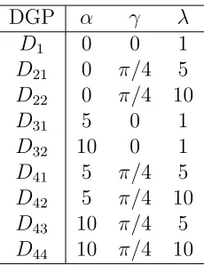
value for nonstationarity (α= 5,10) and for anisotropy ratio (λ= 5,10), and sample size (n= 50,100). From the combinations of the true parameter values in the models, we created nine sets of data as given in Table 3.2. D1 was generated from model M1, D21, D22 from model M2 with different λ, D31, D32 from model M3 with different α,
andD41, D42, D43, D44from modelM4 with the combination of differentλ andα. We
assumed the point source to be located at the origin c = (0,0) for model M3 and M4. These nine data sets were generated with two different sample sizes. 100 data
sets were replicated for each of the nine scenarios, and hence a total of 1800 data sets were generated for our simulation study.
3.3.3
Results
First, we compared the covariance functions of nine scenarios with n = 50 given in Table 3.2 by computing the Frobenius distances between these nine covariance functions. Frobenius distance can be used to measure the distance between two matrices and to indicate the difference between these matrices. Suppose A = {aij}
Table 3.2: True Parameter Values for Each Data Generation Process
DGP α γ λ
D1 0 0 1
D21 0 π/4 5
D22 0 π/4 10
D31 5 0 1
D32 10 0 1
D41 5 π/4 5
D42 5 π/4 10
D43 10 π/4 5
D44 10 π/4 10
Table 3.3: Frobenius Distance between Covariance Functions of Models Σ1 Σ21 Σ22 Σ31 Σ32 Σ41 Σ42 Σ43 Σ44
Σ1 0 8.350 9.745 10.972 11.032 11.120 11.132 11.128 11.133
Σ21 0 2.165 4.810 4.887 4.951 4.979 4.970 4.980
Σ22 0 3.407 3.487 3.413 3.448 3.437 3.450
Σ31 0 0.802 1.721 1.694 1.692 1.689
Σ32 0 1.767 1.741 1.707 1.705
Σ41 0 0.302 0.224 0.312
Σ42 0 0.119 0.076
Σ43 0 0.092
Σ44 0
distance between these two matrices is calculated as,
F(A, B) =
v u u t
n
X
i=1
n
X
j=1
(aij −bij)2. (3.12)
Thus the closerF(A, B) is to 0, then the more these two matricesAandB are similar. Also notice thatF(A, B) = 0 if and only if A=B.
Table 3.3 presents the Frobenius distances between the covariance functions of nine scenarios generated using sample size n = 50. Here, Σi represents the
small between the covariance functions generated from the same model with different parameter values, in particular, between the covariance functions of nonstationary models. Σ1 seemed very different from all of other covariance functions. Σ22 was a
little closer than Σ21 to the covariance functions of the nonstationary models. That
is, the stationary anisotropic model with a large anisotropy ratio (λ= 10) seems to be closer than the stationary anisotropic model with a small anisotropy ratio (λ = 5) to the nonstationary model. The distances of the stationary covariance functions from the nonstationary point source isotropic covariance functions are very similar to those from the nonstationary point source anisotropic covariance functions. Unlike in the stationary models, whether the covariance function is isotropic or anisotropic seemed not to make much difference in the nonstationary models. The stationary anisotropic model appeared closer to the nonstationary models than to the stationary isotropic model. The distances between nonstationary point source isotropic models and non-stationary point source anisotropic models were the smallest among the distances between different models. Similar comparative features are observed between covari-ance functions generated using the sample of size n= 100.
Each of the nine scenarios was modeled using one of four different models,M1,M2, M3, M4. Each dataset was thus modeled with one correct model and three incorrect
Table 3.4: Penalty Given by Each Criterion to Four Models with Two Different Sample Size
n= 50 n = 100
M1 M2 M3 M4 M1 M2 M3 M4
AIC 6 10 8 12 6 10 8 12
BIC 11.736 19.560 15.648 23.472 13.816 23.026 18.421 27.631 AICc 6.522 11.364 8.889 13.953 6.250 10.638 8.421 12.903
different. Only the penalty of AIC does not depend on the sample size n.
We examined whether AIC, AICc, and BIC can correctly identify the true un-derlying model when various spatial models are fit to a particular data set which is generated from one of the models fitted. Results are summarized in Tables 3.5-3.8. Each table presents the percentage of times one of the four models is chosen by an information criterion. For example, the first row and second column of Table 3.4 presents the percentage of times that model M1 is selected based on AICc when D1
is fitted. The last row of each table represents the total percentage of times that the true model is not picked by the corresponding criteria, which can be called an ‘Error ’. In each table, the true model is marked by ‘* ’ for convenience.
We expected the true model to be chosen most of the time, when the data are fitted to various models including the true model. Results from our simulation study indicated that AIC, AICc, and BIC performed well for some specific spatial models, however these criteria performed poorly as well for some other spatial models.
Table 3.5 presents results for D1 generated from the stationary isotropic model, M1. All criteria performed well for both n = 50 and n = 100. Especially BIC