Munich Personal RePEc Archive
A Time-Space Dynamic Panel Data
Model with Spatial Moving Average
Errors
Baltagi, Badi H. and Fingleton, Bernard and Pirotte, Alain
18 April 2018
Online at
https://mpra.ub.uni-muenchen.de/86371/
A Time-Space Dynamic Panel Data Model
with Spatial Moving Average Errors
Badi H. Baltagia, Bernard Fingletonb and Alain Pirottec
aDepartment of Economics and Center for Policy Research, Syracuse University,
United States
bDepartment of Land Economy, University of Cambridge, United Kingdom
cCRED, University Paris II Panthéon-Assas, France
April 18, 2018
Abstract
This paper focuses on the estimation and predictive performance of several esti-mators for the time-space dynamic panel data model with Spatial Moving Aver-age Random E¤ects (SMA-RE) structure of the disturbances. A dynamic spatial Generalized Moments (GM) estimator is proposed which combines the approaches proposed by Baltagi, Fingleton and Pirotte (2014) and Fingleton (2008). The main idea is to mix non-spatial and spatial instruments to obtain consistent estimates of the parameters. Then, a forecasting approach is proposed and a linear predictor is derived. Using Monte Carlo simulations, we compare the short-run and long-run e¤ects and evaluate the predictive e¢ciencies of optimal and various suboptimal predictors using the Root Mean Square Error (RMSE) criterion. Last, our ap-proach is illustrated by an application in geographical economics which studies the employment levels across 255 NUTS regions of the EU over the period 2001-2012, with the last two years reserved for prediction.
Keywords: Panel data; Spatial lag; Error components; Time-space; Dynamic; OLS; Within; GM; Spatial autocorrelation; Direct and indirect e¤ects; Moving average; Prediction; Simulations, Rook contiguity, Interregional trade.
JEL classi…cation: C23.
1
Introduction
There is a growing literature dedicated to dynamic spatial panels, see El-horst (2012, 2014), Lee and Yu (2010, 2015) for a review. Dynamic spatial panels are able to deal with unobservable spatial, individual and/or time speci…c e¤ects. They also tackle more e¢ciently endogeneity problems, such as the potential bias in the coe¢cient of the spatial lag of the dependent vari-able. Baltagi, Fingleton and Pirotte (2014) propose a dynamic spatial model that allows for time dependence as well as spatial dependence, but restricts the time-space covariate to zero along the lines of Franzese and Hays (2007), Kukenova and Monteiro (2009), Jacobs, Ligthart and Vrijburg (2009), Korni-otis (2010), Elhorst (2010), and Brady (2011) to mention a few. They focus on several estimators for the dynamic and autoregressive spatial lag panel data model with spatially correlated disturbances. In the spirit of Arellano and Bond (1991) and Mutl (2006), a dynamic spatial Generalized Method of Moments (GM) is proposed including the Kapoor, Kelejian and Prucha (2007, hereafter KKP) approach for the Spatial AutoRegressive (SAR) error term. The remainder term of the latter is assumed to have a random e¤ects structure. This means that the disturbances are characterised by a SAR-RE process. The main idea is to mix non-spatial and spatial instruments to ob-tain consistent estimates of the parameters. Their Monte Carlo study …nds that when the true model is a dynamic …rst order spatial autoregressive spec-i…cation with SAR-RE disturbances, estimators that ignore the endogeneity of the spatial lag of the dependent variable and endogeneity of the tempo-rally lagged dependent variable perform badly in terms of bias and RMSE. Accounting for spatial correlation in the disturbances also reduces bias and RMSE. Thus, ignoring both sources of spatial dependence leads to a huge bias in the estimated coe¢cients.
especially in the Bayesian Markov Chain Monte Carlo (MCMC) approach. Lee and Yu (2016) consider a spatial Durbin dynamic model which includes simultaneously time dependence, spatial dependence and time-space depen-dence on the explanatory variables. They focus on identi…cation issues and show that parameters are generally identi…ed via Two-Stage Least Square (2SLS) moment relations.
Following this literature, this paper employs a time-space speci…cation as de…ned by Anselin (2001, p. 318), i.e. including a temporal lag (capturing time dependence), a spatial lag (that accounts for spatial dependence), a cross-product term re‡ecting the time-space di¤usion of the dependent vari-able. Many theoretical and/or applied papers are based on this structure, building on a priori theory which does not call for WXs in the model, see Yu, de Jong and Lee (2008), Parent and LeSage (2010, 2011, 2012), Lee and Yu (2014) or Yang (2017) among others. Additionally, the disturbances are assumed to follow a Spatial Moving Average (SMA) process (local spatial spillover e¤ects) in the spirit of Fingleton (2008a). Fingleton (2008b) shows that the sharp cut-o¤ of the SMA disturbances speci…cation is moderated by the spatial lag element of the model. In the cross-section case, when the model contains a spatial lag dependent variable, Kelejian and Prucha (1998, 1999) suggest a 2SLS procedure. They propose that the instrument set should be kept to a low order to avoid linear dependence and retain a full column rank for the matrix of instruments, and thus recommend that (X;WNX) should be used, if the number of regressors is large. Inclusion of spatial lags on the explanatory variables could have a major impact on the performance of the estimation procedure if one were to keep to this rec-ommendation. Pace, LeSage and Zhu (2012) show that the instrumental variables estimation su¤ers greatly in situations where spatial lags of the explanatory variables (WNX) are included in the model speci…cation. The
reason is that this requires the use of (W2NX;W3NX; : : :) as instruments, in place of the conventional instruments that rely onWNX, and this appears to
estimation identi…ed by Pace, LeSage and Zhu (2012). Naturally the choice of this speci…cation would carefully examine the nature of the local spillovers in order to establish their appropriateness for the empirical application at hand.
This paper proposes a spatial GM estimator following the work of Arel-lano and Bond (1991), Mutl (2006) and KKP (2007). Using Monte Carlo simulations, we compare the empirical performance of our GM spatial esti-mator with that of OLS, Within and GMM à la ‘Arellano and Bond’. The latter estimators are panel data estimators that take no account of the spa-tial structure of the disturbances, especially on short-run and long-run e¤ects. We also compare our spatial estimator to other misspeci…ed spatial GM esti-mators, such as that of Mutl (2006). Moreover, forecasting with spatial panel has become recently an integral part of the empirical work in economics, see Baltagi and Li (2004, 2006), Longhi and Nijkamp (2007), Kholodilin, Siliv-erstovs, and Kooths (2008), Fingleton (2009), Schanne, Wapler and Weyh (2010), Girardin and Kholodilin (2011) and Baltagi, Fingleton and Pirotte (2014) among others. We develop a dynamic spatial predictor and evalu-ate the predictive e¢ciencies of various suboptimal predictors relative to the Root Mean Square Error (RMSE) criterion along the lines of Kelejian and Prucha (2007). The plan of the paper is as follows: Section 2 presents the model, section 3 focuses on our spatial GM estimator. Section 4 derives a lin-ear predictor. Section 5 describes the Monte Carlo design. Section 6 presents the simulation results, Section 7 illustrates our approach using an application in geographical economics which studies employment levels across 255 NUTS regions of the EU over the period 2001-2012, with estimation to 2010 and out-of-sample prediction for 2011 and 2012. The last section concludes.
2
The Time-Space Dynamic Panel Model with
SMA Errors
assume that the (N 1)vector yt, whereN is the number of individuals or
regions, at time t will persist at dynamically stable levels so that yt =yt 1
unless there are changes in factors that a¤ect the level of yt. For example
there may be changes in explanatory variables xt, wherext = (x1t; : : :,xN t)>
is an(N K)matrix of explanatory (exogenous) variables, or other changes, such as in unobservable e¤ects. If such a disturbance occurs at time t and is ephemeral, then yt6=yt 1 but given a subsequent period of quiescence as
t ! T then once again we expect yt to converge on a new equilibrium at which yT = yT 1: Assume data are observed where yt 6= yt 1 but tending
to converge, so that yt=f(yt 1), and an autoregressive process is assumed,
hence
yt=&+ yt 1, (1)
in which & is an (N 1)vector and is a scalar parameter. In the long-run with j j<1;and with no subsequent disturbances, the process converges to
yT = 1& .
Consider next connectivity between individuals or regions in the form of a matrix WN, which is a time-invariant (N N) matrix. For purposes of interpreting parameter estimates we normalize WN. This can be done in several ways, for instance by dividing WN by the maximum eigenvalue of WN to give1 W
N, or by dividing each element of WN by its row sum.
Either of these normalizations gives the maximum eigenvalue of WN equal
to 1, and the continuous range for which (IN 1WN) is nonsingular is
1
min(eig) < 1 < max(1eig) = 1, in which 1 is a scalar spatial autoregressive
parameter:
Given (1), logic dictates that
1WNyt = 1WN&+ 1WN yt 1. (2)
Subtracting (2) from (1) leads to another logically consistent expression in which the spatial dependence implied by (2) can be seen in (3) as an explicit cause of variation in yt. Thus
yt 1WNyt =&+ yt 1 ( 1WN&+ 1WN yt 1),
(IN 1WN)yt= ( IN 1 WN)yt 1+ (IN 1WN)&.
1The matrix W
N comprises …xed (non-stochastic) non-negative values with zeros on
Writing = 1 gives
yt=BN1[CNyt 1+BN&], (3)
in which BN = (IN 1WN);CN = ( IN + WN) in which is the au-toregressive time dependence parameter, 1 is the spatial lag coe¢cient, is the time-space di¤usion parameter and IN is an identity matrix of order N. In order to solve equation (3), given appropriate parameter restrictions, equation (3) converges to yT = (BN CN) 1BN&:
Introducing the additional covariates by writing BN& = (x ); in which
is a(k 1)vector, gives
yt=BN1[CNyt 1+x ].
In order to maintain dynamically stable simulations, following Elhorst (2001, 2014, p. 98), Parent and LeSage (2011, p. 478, 2012, p. 731) and Debarsy, Ertur and LeSage (2012, p. 162), requires the largest characteristic root (eigmax) of BN1CN to be less than 1. This restriction ensures that yt
converges to equilibrium levels yT = (BN CN) 1(x ).
Additional realism is introduced as follows. First, the restriction that = 1 is removed since 1 and are unknown, so that is free to vary.
However we anticipate that b b1b: Second, the time invariant matrix x
is replaced by time-varying matrix2 x
t:Third, unobservables are represented
by the error term "t. Although the system may, depending on BN1CN, still
tend towards equilibrium, equilibrium will be continuously disturbed and new equilibrium levels established as t varies. For simplicity of estimation, inter-regional connectivity is assumed to remain constant over the estima-tion period. These consideraestima-tions lead to the time-space dynamic panel data model for i= 1; : : : ; N; t= 1; : : : ; T, which takes the form
yit = yit 1+ 1wiyt+ wiyt 1+xit +"it, (4)
where "it is an error term for region i at time t and wi = (wi1; : : : ; wiN)
is a (1 N) vector which corresponds to the ith row of the matrix WN.
In contrast to the classical literature on panel data, grouping the data by periods rather than units is more convenient when we consider the spatial dimension. For each period t, we have
yt = yt 1+ 1WNyt+ WNyt 1+xt +"t,
[ CNL+BN]yt = xt +"t, (5)
2We assume that the elements ofX
where"t= ("1t; : : : ; "N t)>is an(N 1)vector andLis the time-lag operator,
i.e. Lyt=yt 1. BN is a nonsingular matrix, andBN1 is uniformly bounded. For (5) and following Elhorst (2001, p. 131), Parent and LeSage (2011, p. 478, 2012, p. 731) and Debarsy, Ertur and LeSage (2012, p. 162), stationarity conditions are satis…ed only if CNBN1 <1, which requires
+ ( 1+ )rmax <1 if 1+ 0, (6)
+ ( 1+ )rmin <1 if 1+ <0, (7)
( 1 )rmax > 1 if 1 0, (8)
( 1 )rmin > 1 if 1 <0, (9)
where rmin and rmax are the minimum and maximum eigenvalues of WN.
We allow for a general spatial-autoregressive-moving-average errors process
"it = "it 1+ 2mi"t+uit miut, (10)
where 2 and are respectively autoregressive and moving average
parame-ters, and mi = (mi1; : : : ; miN) is a (1 N) vector which corresponds to the ith row of the spatial matrixMN. MN is similar toWN in that it de…nes the
interaction assumed between the disturbances attributed to di¤erent regions, and it is often the case that MN =WN is assumed. Estimating , 2 and
jointly could be prohibitively di¢cult, and the most widely-used approach to modelling spatial error dependence is a restricted version of this in which
= 0 and = 0, so that
"it = 2wi"t+uit, (11)
in which the autoregressive parameter space must be de…ned so that (IN 2WN)is non-singular, see LeSage and Pace (2009, pp. 88-89). (11) is
referred to as a Spatial AutoRegressive (SAR) process and implies complex interdependence between locations, so that a shock at location j is transmit-ted to all other locations. The SAR process is known to transmit the shocks globally.
In contrast, the Spatial Moving Average (SMA) process, which is the focus of this paper, is obtained by the restrictions = 0 and 2 = 0, hence
so that a shock at locationj will only a¤ect the directly interacting locations given by the non-zero elements in WN. Hence shock-e¤ects are local rather
thanglobal. Regarding the error components,time dependency is introduced
in the innovation uit by specifying an unobserved permanent unit-speci…c
error component i together with the transient error component vit. Thus, uit follows an error component structure
uit = i+vit, (13)
where i is an individual speci…c time-invariant e¤ect which is assumed to be iid 0; 2 , andvit is a remainder e¤ect which is assumed to beiid(0; 2v). i and vit are independent of each other and among themselves. Combining
(12) and (13), we obtain the SMA-RE speci…cation of the disturbance "it.
For a cross-section t, we have
"t =HNut, (14)
with
ut = +vt, (15)
where HN = (IN WN), and ut = (u1t; : : : ; uN t)>, = ( 1; : : : ; N)
>
,
vt= (v1t; : : : ; vN t)> are three vectors of dimension (N 1).
By rewriting the model (5) as
yt=BN1CNyt 1+BN1xt +BN1"t, (16)
the matrix of partial derivatives of yt with respect to the kth explanatory variable of xt in unit 1 up to unit N at timet is given by
h @y
@x1k
@y
@xN k i
t = kB
1
N , (17)
where
BN1 = (IN 1WN) 1 =IN + 1WN + 21W2N + 31W3N + . (18)
The expression (17) denotes the e¤ect of a change of an explanatory variable in a particular spatial unit on the dependent variable of all other units in the short-term. Similarly, the long-term e¤ects are obtained by
h @y
@x1k
@y
@xN k i
= k[ CN +BN] 1
= k[(1 )IN ( 1+ )WN] 1
where
BN 1 = (IN 1WN) 1, 1 =
1+
1 and k =
k
1 . (20)
The expressions in (17) and (19) illustrate that they depend respectively on one and two global spatial multiplier matrices, respectively. Moreover, short-term indirect e¤ects do not occur if 1 = 0, while long-term indirect e¤ects
do not occur if 1 = .
3
A Four Stage Spatial GM Estimator
The presence of a spatial lag, a time-lagged and a time-space lag depen-dent variable renders the usual panel data estimators that ignore this spatial correlation biased and inconsistent. In this context, Instrumental Variables (IV) or GM estimators are required. These estimators assume much weaker assumptions about the initial conditions compared to those of Maximum Likelihood (ML). The consistency of ML estimators depends on the initial conditions and on the way in which the time dimension T and number of cross-sections N tend to in…nity. For dynamic panel data models, Bond (2002) argues that the distribution of the dependent variable depends in a non-negligible way on what is assumed about the distribution of the initial conditions. For example, the initial condition could be stochastic or non-stochastic, correlated or uncorrelated with the individual e¤ects, or have to satisfy stationarity properties. Di¤erent assumptions about the nature of the initial conditions will lead to di¤erent likelihood functions, and the resulting ML estimators can be inconsistent when the assumptions on the initial con-ditions are misspeci…ed, see Hsiao (2003, pp. 80-135) for more details. IV or GM estimators require much weaker assumptions. Following Anderson and Hsiao (1981, 1982) and Arellano and Bond (1991), the individual e¤ect i in (13), which is correlated with the spatial lag and time-lagged dependent variable, is eliminated by …rst-di¤erencing the model (4) yielding
yit= yit 1+ 1wi yt+ wi yt 1+ xit + "it; (21)
t = 2; : : : ; T, and for a cross-section t, we have
yt= yt 1+ 1WN yt+ WN yt 1 + xt + "t. (22)
Following (14) and (15), (22) can be written as
Following Arellano and Bond (1991), we can de…ne a GM estimator based on the assumption of no correlation between the …rst-di¤erenced disturbances and earlier time-lagged levels of the dependent variable, yit 1. This yields
the following moment conditions:
E(yil vit) = 0; 8i; l = 0;1; : : : ; t 2; t= 2; : : : ; T. (24)
If we assume that the explanatory variablesxk;im are strictly exogenous3, the
following additional moment conditions can be used
E(xk;im vit) = 0; 8i; k; m= 1; : : : ; T;t = 2; : : : ; T. (25)
If, xk;im is weakly exogenous then the associated moment conditions are
E(xk;im vit) = 0; 8i; k; m= 1; : : : ; t 1; t= 2; : : : ; T. (26)
Moreover, to take into account the endogeneity of the spatial lag, we can use spatially weighted earlier time-lagged levels of the dependent and explana-tory variables as instruments. This strategy is associated with the following moments conditions:
E(wiyl vit) = 0; l= 0;1; : : : ; t 2; t= 2; : : : ; T, (27)
E(wiyl vit) = 0; l= 0;1; : : : ; t 2; t= 2; : : : ; T, (28)
E(wixk;m vit) = 0; 8i; k; m= 1; : : : ; T; t= 2; : : : ; T, (29)
E(wixk;m vit) = 0; 8i; k; m= 1; : : : ; T; t= 2; : : : ; T, (30)
where wi = (wi1; : : : ; wiN) is a(1 N) vector which corresponds to the ith row of the matrix W2N. Considering the weakly exogenous assumption of
xk;im, the moment conditions (29) and (30) are replaced by the following:
E(wixk;m vit) = 0; 8i; k; m= 1; : : : ; t 1; t= 2; : : : ; T, (31)
E(wixk;m vit) = 0; 8i; k; m= 1; : : : ; t 1; t= 2; : : : ; T. (32)
Let us de…ne the matrix Z which contains the non-spatial instruments (i.e. related to the conditions (24) and (25)) as
Z=diag(Z2;Z3; : : : ;ZT), (33)
where
Zt= (y0;y1; : : : ;yt 2;x1; : : : ;xT) (34)
is an (N [(t 1) +KT]) matrix of instruments at time t, yl is a vector of
dimension (N 1) and xr is a matrix of dimension(N K). Moreover, we can de…ne a matrix Zs which contains the spatial instruments (i.e. related to the conditions (27), (28), (29) and (30)) as
Zs=diag(Zs2;Zs3; : : : ;ZsT), (35)
with
Zst = (yst;yts ;xs;xs ), (36)
where yst = y0s;ys1; : : : ;yst 2 , yst = y0s ;ys1 ; : : : ;yts 2 , xs = (xs1; : : : ;xsT),
xs = (xs1 ; : : : ;xsT ), and
ysl =
0 B B B @
w1yl
w2yl
.. .
wNyl 1 C C C
A=WNyl, y s l = 0 B B B @
w1yl
w2yl
.. .
wNyl 1 C C C A=W
2
Nyl, (37)
where yl= (y1l; : : : ; yN l)> and
xsr =
0 B B B @
w1x1r w1x2r w1xKr
w2x1r w2x2r w2xKr
..
. ... ...
wNx1r wNx2r wNxKr
1 C C C
A=WNxr, (38)
xsr =
0 B B B @
w1x1r w1x2r w1xKr
w2x1r w2x2r w2xKr
..
. ... ...
wNx1r wNx2r wNxKr
1 C C C A=W
2
Nxr, (39)
where xkr= (xk1r; : : : ; xkN r)>,k = 1; : : : ; K. If we stack the matrices Z and
Zs, we obtain the valid instruments for the model (21), namelyZ . Moreover, we use the weight matrix of moments
AN =
h
EhZ >( ") ( ")>Z ii
1
with
Eh( ") ( ")>i= 2v HNH>N , (41)
where = 0 B B B B B B B @
2 1 0 0 0
1 2 1 0 0
0 1 . .. ... ... ...
... ... ... ... 1 0
0 0 0 1 2 1
0 0 0 1 2
1 C C C C C C C A , (42)
is the variance-covariance matrix of the remainder MA(1) unit roots error which is of dimension (T 1 T 1)used by Arellano and Bond (1991) in their one-step GMM estimator.
A consistent estimate of the parameters and 2
v can be obtained using
a GM approach in the spirit of Fingleton (2008a) for the static spatial lag model including a SMA-RE process on the disturbances. In fact, Fingleton (2008a) extended the GM procedure from panel data proposed by KKP (2007) for the SAR-RE case to the SMA-RE one. Here, the main di¤erence is that we base the estimation of and 2
v on the …rst di¤erences of the errors to
account for the dynamics and to get rid of the individual e¤ects. Following the derivation of the moment conditions and ignoring the expectations of each term, the system involving and 2
v can be expressed as
N gN =0, (43)
where
N = 0 @ 2
N(T 1) 2 (T 1)t1 0
2 (T 1)t1 2 (T 1)t2 4 (T 1)t3
0 2 (T 1)t3 2 (T 1) (t1+t4)
1 A, =
0 @ 2 v 2 2 v 2 v 1 A,
gN =
0
@ "
> "
"> "
"> "
1
A, (44)
with t1 =tr WN>WN , t2 =tr (W2N)
>
WN2 , t3 =tr (W2N)
>
WN , t4 =
tr(W2N)>. The GM estimators of and 2 are the solution of the
(2008a) for the static spatial lag model including a SMA-RE process for the disturbances. Our spatial GM procedure comprises of the following four steps:
In the …rst step, we use an IV or GM estimator to get consistent esti-mates of , 1, and .
In the second step, the IV or GM residuals are used to obtain consistent estimates of the moving average parameter and the variance 2
v.
In the third step, we compute the preliminary one-stage consistent Spatial GM estimator which is given by
b1 = ( Xe>Z AbNZ > Xe) 1 Xe>Z AbNZ > y, (45)
where Xe = y 1;(IT 1 WN) y,(IT 1 WN) y 1, x , > 1 =
; 1; ; > and
b
AN =hZ > HbNHb>N Z i 1, (46)
with HbN = (IN bWN).
In the fourth step, following Arellano and Bond (1991), we replace (46) by its robust version
VN =
h
Z > IT 1 HbN IT 1 Hb>N Z
i 1
(47)
where
=h( v) ( v)>i (JT 1 IN), (48)
andJT 1 = T 1 >T 1 , T 1is a vector of ones of dimension(T 1 1).
To operationalize this estimator, v is replaced by di¤erenced resid-uals obtained from the preliminary one-stage consistent Spatial GM estimator (45). The resulting estimator is the two-stage Spatial GM estimator
4
Prediction
In 2014, Baltagi, Fingleton and Pirotte argued that the derivation of the predictor for a dynamic autoregressive spatial panel data model is more complicated because the time/space lags of the dependent variable are corre-lated with the disturbances. Thus, the Goldberger (1962) framework, which assumes no correlation between the regressors and the error term, is not applicable in this context. The predictor proposed by Baltagi, Fingleton and Pirotte (2014), under the restrictive assumption of no time-space de-pendence and SAR-RE disturbances structure, depends on the process that generates the initial values and this may be di¢cult to handle in practice. So, here, considering (4) without any restriction on time-space dependence and a SMA-RE process on the disturbances"which captures local spillovers, we propose a tractable approach which does not depend explicitly on the ini-tial values. In the …rst step, the individual e¤ects are estimated from the residuals observed over time. To obtain this, we commence by using a single cross-section equation at time t, in particular
yt = 1WNyt+CNyt 1+xt +"t. (50)
So that
"t=HNut=yt 1WNyt CNyt 1 xt , (51)
and
ut = +vt =HN1(yt 1WNyt CNyt 1 xt ), (52)
=HN1(BNyt CNyt 1 xt ) vt, (53)
with vt N(0; 2vIN). In order to calculate b, one uses observed data for
the sequence of ys in equation (53) together with the parameter estimates (b,b1,b,b,b,b2v,b2), using the data for the period t= 2; : : : ; T (assuming that
y0 is not available) on each occasion drawing an(N 1)vectorvtat random
from theN 0;b2vIN distribution. This gives T 1di¤erent estimates of b,
so we take the time mean as an estimate of the time-invariant(N 1)vector , given E[vt] =0. Also, the estimate is scaled so that its variance is equal
to b2. So, here, it is necessary to estimate 2 and not only and 2
v. These
level residuals are used to obtain consistent estimates of the moving average parameter and the variances 2
v and 2. In the second step, this estimated
, denoted by , is then used in a bootstrap forecast approach considering observed values yT for the …rst forecastybT+1;and estimates of futurebyfrom
then on. Thus, the predictor is given by
b
yt=BbN1hCbNbyt 1+xtb+HbN i, (54)
which solves recursively over t = T + 1; T + 2; : : : ; T + , 1 with yT
replacing ybT for t=T + 1. In the Monte Carlo experiments that follow, this
predictor (54) is compared to other suboptimal predictors which correspond to misspeci…ed dynamic estimators.
5
Monte Carlo Design
We assume that the dependent variable yit, i = 1; : : : ; N; t = 1; : : : ; T, is
given from a spatial dynamic panel data model of the form
yit=a+ yit 1+ 1wiyt+ wiyt 1+ xit+"it, (55)
where the disturbance "it follows a SMA process
"it =uit wiut, (56)
wi = (wi1; : : : ; wiN)is a(1 N) vector which corresponds theith row of the
matrix WN, = 0:4, since this equates to positive dependence, anduit has
an error component structure
uit = i+vit, (57)
with i iid:N 0; 2 ,vit iid:N(0; 2v)and 2; 2v = (0:8;0:2);(0:2;0:8).
The explanatory variable xit is generated as
xit= xit 1+ it, (58)
with = 0:8, it iid:N 0; 2 and 2 = 10. We setx
i; 50= 0 and generate
xit for t= 49; 48; : : : ; T. Foryit, we also setyi; 50 = 0 and discarded the
…rst 51 observations, using the observations t = 1 through T for estimation (we assume thaty0 is non available in order to be closer to the empirical
For the coe¢cients of (55), we take (a; ; 1; ; ) = (1;0:2;0:8; 0:2;1), (1;0:8;0:4; 0:3;1), (1;0:7;0:8; 0:6;1) and (1;0:8;0:8; 0:7;1). Moreover, following Baltagi and Yang (2013), the spatial matrix WN has a rook
conti-guity structure4. This matrix is generated as follows: (i) index theN spatial
units by 1; :::; N. Randomly permute these indices and then allocate them into a lattice of R M( N) squares. (ii) let wi;j = 1 if the index j is
in a square which is on the immediate left, or right, or above, or below the square which contains the index i, otherwise wi;j = 0; and (iii) divide each
element of WN by its row sum. For all experiments, 5;000 replications are
performed. We compute the mean, standard deviation, bias and RMSE of the coe¢cientsb,b1,b,b,band the average direct, indirect and total short-term and long-short-term e¤ects using respectively (17) and (19). Following KKP (2007), we adopt a measure of dispersion which is closely related to the stan-dard measure of root mean square error (RMSE), but is based on quantiles. It is de…ned as
RMSE=
"
bias2+ IQ
1:35
2#1=2
, (59)
where bias is the di¤erence between the median and the true value of the parameter, and IQ is the interquantile range de…ned as c1 c2 where c1
is the 0.75 quantile and c2 is the 0.25 quantile. Clearly, if the distribution
is normal the median is the mean and, aside from a slight rounding error, IQ/1.35 is the standard deviation. In this case, the measure (59) reduces to the standard RMSE.
We compare the performance of 5 estimators in our Monte Carlo experi-ments. These are as follows:
1. Ordinary Least Squares (OLS) which does not deal with the endogene-ity of the spatial lag WNy, the time lag y 1 and the time-space lag
WNy 1. OLS also ignores the SMA-RE process generating the
distur-bances.
2. The Within estimator which wipes out the individual e¤ects, but oth-erwise does not deal with the endogeneity of the spatial lagWNy, the
time lag y 1 and the time-space lagWNy 1 nor the SMA process for the disturbances.
4Following Kelejian and Prucha (1999), we have also considered the spatial matrix
which is labelled as “j ahead andjbehind” with the non-zero elements being1=2j,j= 2,
3. The Arellano and Bond (1991) GMM estimator which eliminates the individual e¤ects by di¤erencing, and handles the presence of the lagged dependent variable by using the orthogonality conditions (24) and (25). However, this estimator ignores the spatial lag WNy, the time-space
lag WNy 1 and the SMA process for the disturbances.
4. GM-TS-RE is an estimator that uses the orthogonality conditions (24) and (25) of Arellano and Bond (1991) as well as the spatial orthog-onality conditions (27), (28), (29) and (30). However, this estimator ignores the SMA process for the disturbances.
5. GM-TS-SMA-RE is an estimator that uses the orthogonality condi-tions (24) and (25) of Arellano and Bond (1991) as well as the spatial orthogonality conditions (27), (28), (29) and (30) used by GM-TS-RE, but it also accounts for the SMA structure of the disturbances using a similar approach to that of Fingleton (2008a), see Section 3.
Last, for each experiment, we use the post sample RMSE criterion and compute the out of sample forecast errors for each predictor associated with the alternative estimators for one to …ve step ahead forecasts. In order to do this, we generate 5 more time periods for each individual (i.e. T + , = 1; : : : ;5) which are not used in the estimation. An average RMSE is also calculated across all individuals at di¤erent forecast horizons.
6
Monte Carlo Results
The estimates obtainedviathe various estimators are summarised in Tables 1
to 4(N = 100)and 6 to 9(N = 200). They report the mean, bias and RMSE
of b,b1,b,band bgiven various assumed true values for the data generating
process. The di¤erence between Tables 1 and 2 (resp. Tables 5 and 6) is that in Table 2 (resp. Table 6) we assume greater individual heterogeneity where 2 = 0:8rather than0:2. This is done holding the total variance of the
disturbances constant, i.e., 2+ 2
v = 1 in both Tables. Tables 1 and 2 (resp.
Tables 5 and 6) show clearly that the GM-TS-SMA-RE estimator has the lowest RMSEs for all experiments considered. This is especially true when the individual heterogeneity and is high, i.e. when 2; 2
v = (0:8;0:2)
rather than 2; 2
v = (0:2;0:8). When N increases, comparing Tables 1
perfom better in terms of RMSE. Table 11 reports the mean RMSE and it clearly shows that GM-TS-SMA-RE performs well compared to the other estimators. Tables 3 and 4 (resp. Tables 7 and 8) give the RMSE variation for direct, indirect and total long and short-term e¤ects in the case of the two GM-based spatial estimators.
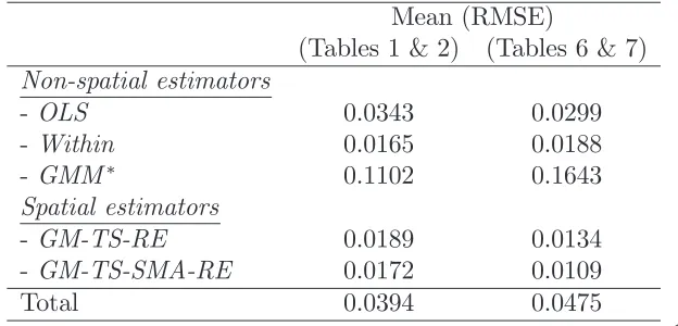
[image:19.595.143.455.279.429.2][INSERT TABLES 1 TO 10]
Table 11 - Mean RMSE for the non-spatial and spatial estimators
Mean (RMSE)
(Tables 1 & 2) (Tables 6 & 7) Non-spatial estimators
- OLS 0.0343 0.0299
- Within 0.0165 0.0188
- GMM 0.1102 0.1643
Spatial estimators
- GM-TS-RE 0.0189 0.0134
- GM-TS-SMA-RE 0.0172 0.0109
Total 0.0394 0.0475
This estimator does not consider RMSEs of the coe¢cients b1 and b.
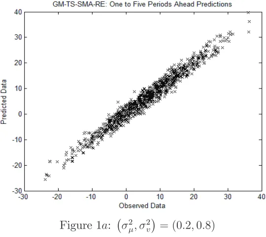
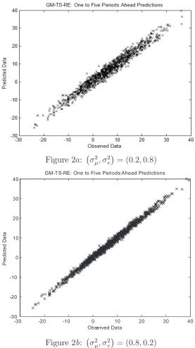
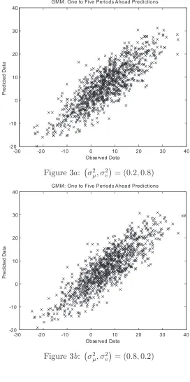
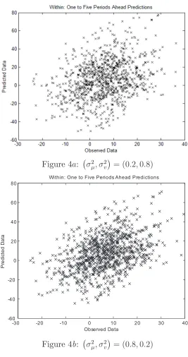
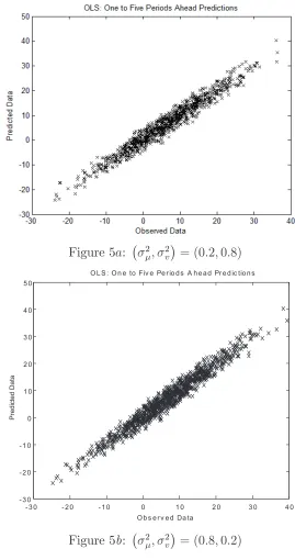
In order to illustrate the comparative prediction performance, Figures 1a to 5a and 1b to 5b show outcomes from speci…c parameter assump-tions considering (N; T) = (200;12). In particular, Figures 1a to 5a, use (a; ; 1; ; ; ) = (1;0:2;0:8; 0:2;1; 0:4), 2; 2
v = (0:2;0:8) and =
1; : : : ;5whereas Figures 1b to5b use the same values of (a; ; 1; ; ; ), but allow for a higher level of individual heterogeneity, i.e. 2; 2
v = (0:8;0:2).
Figure1b shows the good performance associated with the GM-TS-SMA-RE compared to the other …gures. This …gure also shows that the higher the individual heterogeneity, i.e. 2; 2
v = (0:8;0:2), the better the forecasting
Figure 1a: 2; 2
v = (0:2;0:8)
-30 -20 -10 0 10 20 30 40
-30 -20 -10 0 10 20 30 40
GM-T S-SMA-RE: One to Fi ve Peri ods Ahead Predi cti ons
Observed Data
P
re
d
ic
te
d
D
a
ta
Figure 1b: 2; 2
Figure 2a: 2; 2
v = (0:2;0:8)
-30 -20 -10 0 10 20 30 40
-30 -20 -10 0 10 20 30 40
GM-T S-RE: One to Fi ve Peri ods Ahead Predi cti ons
Observed Data
P
re
d
ic
te
d
D
a
ta
Figure 2b: 2; 2
-30 -20 -10 0 10 20 30 40 -20
-10 0 10 20 30 40
GMM : One to Fi ve Peri ods Ahead Predi cti ons
Observed Data
P
re
d
ic
te
d
D
a
[image:22.595.155.427.158.703.2]ta
Figure 3a: 2; 2
v = (0:2;0:8)
-30 -20 -10 0 10 20 30 40
-20 -10 0 10 20 30 40
GM M: One to Fi ve Peri ods Ahead Predi cti ons
Observed Data
P
re
d
ic
te
d
D
a
ta
Figure 3b: 2; 2
Figure 4a: 2; 2
v = (0:2;0:8)
-30 -20 -10 0 10 20 30 40
-60 -40 -20 0 20 40 60 80
Within: One to Five Periods Ahead Predi ctions
Observed Data
P
re
d
ic
te
d
D
a
ta
Figure 4b: 2; 2
Figure 5a: 2; 2
v = (0:2;0:8)
- 3 0 - 2 0 - 1 0 0 1 0 2 0 3 0 4 0
- 3 0 - 2 0 - 1 0 0 1 0 2 0 3 0 4 0 5 0
O L S : O n e to Fiv e Pe r io d s A h e a d Pr e d ic tio n s
O b s e r v e d D a ta
P
re
d
ic
te
d
D
a
ta
Figure 5b: 2; 2
7
Empirical Illustration
In this section, we apply the estimation and prediction methods outlined above to estimate a time-space dynamic panel data model in which the level of employment across EU regions observed over recent years is the dependent variable and levels of output and capital are hypothesized causes of employ-ment variation, controlling for spatial and temporal interactions involving employment. We analyze total employment over the period 2001-2010 across
N = 255NUTS2 regions of the EU5. The model speci…cation we adopt is
de-rived from standard urban economics as given by Abdel-Rahman and Fujita (1990), Ciccone and Hall (1996) and Fujita and Thisse (2002), among many others. From this it is possible to derive a model which shows that the drivers of (log) employment (lne) are (log) output denoted by lnq and a measure of (log) capital investment denoted by lnk. Following the arguments made at the start of Section 2, we assume an underlying trend toward equilibrium in employment levels in the absence of any disturbances. In reality equilib-rium will be disturbed by other factors, but we maintain an assumption of a tendency towards equilibrium following a shock, so that lnet =f(lnet 1)
and this leads logically to our speci…cation with temporal and spatial wage interdependence, thus
lnet =c t+ lnet 1+ 1WNlnet+ WNlnet 1+ 1lnqt+ 2lnkt+"t (60)
in which t is a vector of ones of dimension (N 1), et, et 1, qt and kt are
(N 1) vectors of observations in levels, with t= 2001; : : : ;2010. The data series are based on Cambridge Econometrics’ European Regional Economic Data Base, in whichetis the annual regional employment series,qtis output
(Gross Value Added, or GVA) and kt is a measure of capital investment (Gross Fixed Capital Formation, or GFCF). The error term "t captures all
other unobservable e¤ects in‡uencing the level of employment, especially interregional heterogeneity.
Written in …rst di¤erence terms, in other words as exponential growth rates, the estimating equation is
lnet = lnet 1+ 1WN lnet+ WN lnet 1+ 1 lnqt
+ 2 lnkt+ "t. (61)
5We use ’regions of the EU’ as a convenience, since some regions are located in closely
The matrixWN is based on estimated bilateral trade ‡ows between EU
NUTS2 regions. The data come from the PBL (the Netherlands Environ-mental Assessment Agency)6 who developed a new methodology which is
close to that of Simini et al. (2012). Details of the methodology are given in Thiessen et al. (2013a, b, c), see also Gianelle et al. (2014). The method follows a top-down approach and therefore is consistent with the national accounts of the di¤erent countries. Given the total international exports and imports on the country level, interregional trade ‡ows are derived using data on business travel (services) and on freight transport (goods). Trade ‡ows involving regions of Switzerland and Norway were obtained on the basis of interregional trade ‡ows estimated by the best linear disaggregation method of Chow and Lin (1971), which was initially used to break down annual time series into quarterly series (see Abeysinghe and Lee, 1998, Doran and Fin-gleton, 2014). In this, commencing with aggregate trade values7 between
21 EU counties, these were allocated to the NUTS2 regions. A parallel ap-proach has been used by Polasek, Verduras and Sellner (2010), Vidoli and Mazziotta (2010), and Fingleton, Garretsen and Martin (2015), who pro-vide more detail. Finally, OLS regression of the log PBL trade ‡ows on log Chow-Lin trade ‡ows produced parameters used to predict the missing PBL regional trade ‡ows for Switzerland and Norway using the values for these regions obtainedviathe Chow-Lin approach. We subsequently normalize the trade matrix by dividing by its maximum eigenvalue, thus giving the matrix
WN: This normalization ensures that the most positive real eigenvalue of
WN is equal to max(eig) = 1:0, and the continuous range for 1 for which
BN = (IN 1WN) is nonsingular is min(1eig) < 1 < 1. This normalization
retains real trade magnitude di¤erences between regions so thatWN lnet, for example, depend on the size of the trade ‡ow between regions. In contrast, normalization by row standardization would make interregional interaction depend on trade shares.
Assuming an SMA process for the compound errors, the spatial error de-pendence is "it =uit miut in whichmi is thei’th row ofMN, whereMN
is an (N N) row-normalized regional contiguity matrix. The key feature of an SMA process is that shocks to the unobservables have local rather than global e¤ects. Note that both components of the compound errors "t are
6We are grateful to Mark Thiessen, who kindly provided the data. The data can be
visualized at http://themasites.pbl.nl/eu-trade/index2.html?vis=net-scores.
7They are downloadable from http://cid.econ.ucdavis.edu/data/undata/undata.html,
assumed to be subject to this same spatial error dependence processes. The SMA assumption is somewhat distinct from the more usual SAR assump-tion for the errors, which implies complex simultaneous associaassump-tion involving errors across all regions.
With regard to causation, we make two assumptions. One is that the regressors are strictly exogenous. In this case the moments conditions8 are
given by equations (25) and (29), combined with the moments for the en-dogenous variable and its spatial lag, as de…ned in the moments equations (24) and (27). Probably a more realistic assumption is that there will be feedback from employment to the variables qt and kt but that this will be
delayed rather than instantaneous, and thus we estimate the model assuming that the variables are predetermined. In this case estimation is based on the moments (26), (31), (24) and (27).
Columns 1 and 2 of Table 12 gives the resulting parameter estimates9
for equation (61) assuming either predeterminedness or exogeneity, and this shows that the e¤ects of lnqt and lnkt on lnet are signi…cant and positive.
Note that the negative estimated also indicates positive error dependence. If the positive space and time dependence parameter estimates were large, so that + 1 > 1, this would not necessarily imply nonstationarity if <
0. On the other hand given a restriction that = 0 then large would necessarily requires small 1 in order to satisfy stationarity. Therefore under the assumption that = 0the possibility of bias is introduced. However with
6
= 0, in other words with no restriction imposed on space-time covariance, a large positive plus large positive 1 could be o¤set by a negative covariance term so that collectively the parameters pass the stationarity conditions. In this instance it turns out that with predetermined regressors the maximum absolute eigenvalue ofCNBN1 is0:6757<1, 1+ = 0:13472,j j+( 1+ ) =
0:7872<1, and 1 = 0:9359, ( 1 ) = 0:28337> 1, see (6), (7), (8) and (9). Likewise, assuming exogenous regressors, the model parameter estimates indicate stationarity and dynamic stability.
The estimates obtained cast some light on the question of increasing re-turns, in other words as a region’s economy grows, are there productivity
8For simplicity, we exclude the additional moments based onW2
N:
9Note that because the estimates are based on di¤erences, no estimate of the constant
c is provided. This estimate is subsequently constructed as the di¤erence between lne
and the expected lne given by the model without c, using means over time. With the
assumption of predetermined regressors this gives c= 0:4462;assuming exogeneity gives
bene…ts so that employment grows by less than output, due to positive ex-ternalities associated with increasing size and diversity of the economy as
q increases overcoming negative ones such as the e¤ects of congestion. As-suming predetermined regressors, controlling for the e¤ect of k, spatial in-teraction, temporal dependence and space-time covariance, the estimated 1 suggests that a 1% increase inqproduces a0:1272% increase in employment. This would indicate a high level of productivity growth. However, this es-timate is misleading. As noted earlier, under model speci…cations involving autoregressive spatial interdependence of a dependent variable y, the partial derivative @y
@xj is not simply equal to the regression coe¢cient j, as pointed
out by LeSage and Pace (2009). The true e¤ect of xj di¤ers from j because it also includes the consequences of spillovers across regions. Based on the Table 12 estimates, one obtains via equations (17) and (19) (the means of) the true derivatives which are given in Table 13, with total e¤ects partitioned into direct and indirect components. As shown in Table 13 the total long-term total e¤ect of q equal to 0:4184, assuming predetermined regressors, which remains well below the value of 1:0 which one would associate with constant returns to scale. In order to obtain the standard errors and hence t-ratios given in Table 13, we draw at random from the multivariate normal distribution with mean equal to the parameter estimates given in Table 12, and covariance matrix equal to the estimated covariance matrix for these pa-rameters. Each draw allows us to calculate the corresponding short and long term direct, indirect and total e¤ects. With multiple (500) draws we obtain the distributions of these e¤ects thus giving the standard errors in Table 13. From these draws it is evident that the e¤ects are signi…cantly di¤erent to zero under exogeneity and predetermindness. Note that the total long term elasticity with regard to GVA is similar, and clearly less than 1:0, regard-less of estimator. It is evident that increasing productivity is an enduring characteristic of the EU regional economy.
The predictive performance of the SMA speci…cation is given by the one-and two-step ahead predictions10, as measured by the post sample RMSE
criterion. Computing the out-of-sample forecast errors for 2011 and for 2012 indicates that the speci…cation with either predetermined regressors or as-suming exogeneity, provides relatively accurate predictions compared with the outcome of assuming SAR errors, which do not explicitly focus on
lo-10Data limitations mean that for 2012,kin each region is estimated using each region’s
cal spillovers. With SAR errors "it = 2
PN
j=1mij"jt +uit in which mij
denotes cell(i; j) of MN, and uit = i +vit; in which i iid(0; 2) is a
region (i.e. individual)-speci…c time-invariant e¤ect and the remainder ef-fect vit iid(0; 2v). In this case the RMSEs for the SAR errors estimator
are calculated from the di¤erence between yt and byt given by the prediction
equation
b
yt=BbN1 h
b
CNbyt 1+c t+xtb+HbN1 i
(62)
in which HbN = (IN b2MN) is a nonsingular matrix and is based on
=HN(BNyt CNyt 1 xt c t) vt. (63)
With exogenous regressors, the the SAR errors estimator is non-stationary and dynamically unstable with out-of-sample RMSE forecast errors for 2011 and for 2012 of 0:8305 and 2:3758: Assuming predetermined regressors, the estimator is stationary and gives RMSE’s of 0:1742 and 0:2291.
The …nal two columns of Table 12 gives estimates for the SMA errors speci…cation with predetermined and exogenous regressors, but with the additional variables WNx1t, the spatial lag of qt, with parameter 3, and
WNx2t, the spatial lag ofk, with parameter 4. This is thus a form of
spa-tial Durbin speci…cation with regressors xt = (x1t;x2t;WNx1t;WNx2t):The
additional covariates evidently cause a problem of weak instruments, giv-ing dynamically unstable nonstationary estimates, as re‡ected by the largest characteristic roots of BN1CN equal to 1:0663 and 1:9041 respectively, and
the one-step ahead RMSEs are 7:4094 and 3:0746: Assuming the Spatial Durbin with predetermined regressors and with 2 restricted to zero, gives a
largest characteristic root equal to 1:1127 and RMSE equal to 3:3007. The same speci…cation but with a spatial autoregressive (SAR) error process gives 2:489 and 23:3138 respectively. Thus omitting the spatial lags WNx1t and
WNx2t and hence restricting the direct e¤ect to the total e¤ect ratio to
Table 12 - GM-TS-SMA-RE parameter estimates
Parameters Predetermined Exogenous Spatial Durbin Spatial Durbin
(a) (b)
0:6525
(0:003769) (173:1)
0:5634
(0:001425) (395:2)
0:3357
(0:00209) (160:6)
0:5673
(0:002129) (266:4) 1 0:5353
(0:01045) (51:2)
0:5909
(0:006908) (85:54)
1:5160
(0:01156) (131:2)
1:1990
(0:01358) (88:3) 1 0:1272
(0:002116) (60:11)
0:1787
(0:0006129) (291:5)
0:3604
(0:001307) (275:6)
0:1897
(0:001245) (152:4)
2 0:02636
(0:0006568) (40:13)
0:01966
(0:0001589) (123:7)
0:03702
(0:0007463) ( 49:61)
0:01581
(0:0002156) (73:34)
3 _ _ 0:2910
(0:005024) (57:91)
0:3576
(0:006044) (59:18)
4 _ _ 0:3930
(0:003494) ( 112:5)
0:3025
(0:002825) ( 107:1)
0:4006
(0:008868) ( 45:17)
0:3807
(0:005913) ( 64:39)
0:8863
(0:008452) ( 104:9)
0:9465
(0:009802) ( 96:56)
0:7975 0:6545 0:3079 0:5852
2 0:0753 0:2786 0:0097 0:4663
2
v 0:0003 0:0003 0:0006 0:0003
Forecasting RMSE
2011 0:0465 0:1413 7:4094 3:0746
2012 0:0977 0:2168 7:4711 3:1091
Average 0:0721 0:1791 7:4403 3:0918
Table 13 - GM-TS-SMA-RE short- and long-term e¤ects
Predetermined Exogenous
Direct Indirect Total Direct Indirect Total GVA(q)
Short-term 0:1278
(0:00218) (60:94)
0:0285
(0:0007) (38:43)
0:1564
(0:0022) (70:27)
0:1798
(0:0006) (288:43)
0:0473
(0:0009) (51:31)
0:2271
(0:0011) (213:42)
Long-term 0:3669
(0:0068) (53:624)
0:0515
(0:0020) (26:08)
0:4184
(0:0069) (60:90)
0:4108
(0:0008) (494:39)
0:0779
(0:0017) (47:03)
0:4887
(0:0019) (257:59)
GFCF(k)
Short-term 0:0265
(0:0007) (39:67)
0:0059
(0:0002) (24:20)
0:0324
(0:0009) (38:07)
0:0198
(0:0002) (121:60)
0:0052
(0:0001) (46:80)
0:0250
(0:0002) (110:39)
Long-term 0:0760
(0:0017) (44:50)
0:0107
(0:0005) (20:76)
0:0867
(0:0020) (44:27)
0:0452
(0:0004) (117:40)
0:0086
(0:0002) (44:78)
0:0538
(0:0005) (111:81)
8
Conclusion
References
Abdel-Rahman, H. and Fujita, M. (1990). ‘Product variety, Marshallian externalities and city size’, Journal of Regional Science, Vol. 30, pp. 165–83.
Abeysinghe, T. and Lee, C. (1998). ‘Best linear unbiased disaggregation of annual GDP to quarterly …gures: the case of Malaysia’, Journal of Forecasting, Vol. 17, pp. 527-537.
Anderson, T.W. and Hsiao, C. (1981). ‘Estimation of dynamic models with error components’, Journal of the American Statistical Association, Vol. 76, pp. 598-606.
Anderson, T.W. and Hsiao, C. (1982). ‘Formulation and estimation of dynamic models using panel data’, Journal of Econometrics, Vol. 18, pp. 47-82.
Anselin, L. (2001). Spatial econometrics. Ch. 14 in B.H. Baltagi, ed., A Companion to Theoretical Econometrics, Blackwell Publishers Lte, Massachusetts, pp. 310-330.
Anselin, L., Le Gallo, J. and Jayet, H. (2008). Spatial panel econometrics, Ch. 19 in L. Mátyás and P. Sevestre, eds., The Econometrics of Panel Data: Fundamentals and Recent Developments in Theory and Practice, Springer-Verlag, Berlin, pp. 625-660.
Arellano, M. and Bond, S. (1991). ‘Some tests of speci…cation for panel data: Monte Carlo evidence and an application to employment’,Review of Economic Studies, Vol. 58, pp. 277-297.
Arellano, M. and Bover, O. (1995). ‘Another look at the instrumental vari-able estimation of error-components models’. Journal of Econometrics, Vol. 68, pp. 29-52.
Baltagi, B.H. and Li, D. (2006). ‘Prediction in the panel data model with spatial correlation: the case of liquor’, Spatial Economic Analysis, Vol. 1, pp. 175-185.
Baltagi, B.H. and Yang, Z. (2013). ‘Heteroskedasticity and non-normality robust LM tests for spatial dependence’, Regional Science and Urban Economics, Vol. 43, pp. 725-739.
Baltagi, B.H., Fingleton, B. and Pirotte, A. (2014). ‘Estimating and fore-casting with a dynamic spatial panel data model’, Oxford Bulletin of Economics and Statistics, Vol. 76, pp. 112-136.
Blundell, R. and Bond, S. (1998). ‘Initial conditions and moment restrictions in dynamic panel data models’, Journal of Econometrics, Vol. 87, pp. 115-143.
Blundell, R., Bond, S. and Windmeijer, F. (2000). ‘Estimation in dynamic panel data models: improving on the performance of the standard GMM estimator’. Advanced in Econometrics, 15, pp. 53-91.
Bond, S. (2002). ‘Dynamic panel data models: a guide to micro data meth-ods and practice’, Portuguese Economic Journal, Vol. 1, pp. 141-162.
Bouayad-Agha, S. and Védrine, L. (2010). ‘Estimation strategies for a spa-tial dynamic panel using GMM. A new approach to the convergence issue of European regions’, Spatial Economic Analysis, Vol. 5, pp. 205-227.
Brady, R.R. (2011). ‘Measuring the di¤usion of housing prices across space and time’, Journal of Applied Econometrics, Vol. 26, pp. 213-231.
Ciccone, A. and Hall, R. E. (1996). ‘Productivity and the density of eco-nomic activity’, American Economic Review, Vol. 86, pp. 54–70.
Chow, G. and Lin, A.-I. (1971). ‘Best linear unbiased interpolation, dis-tribution and extrapolation of time series by related series’, Review of Economics and Statistics, Vol. 53, pp. 372-375.
Doran, J. and Fingleton, B. (2014). ‘Economic shocks and growth: spatio-temporal perspectives on Europe’s economies in a time of crisis’,Papers in Regional Science, Vol. 93, pp. S137-S165.
Elhorst, J.P. (2001). ‘Dynamic models in space and time’, Geographical Analysis, Vol. 33, pp. 119-140.
Elhorst, J.P. (2010). ‘Dynamic panels with endogenous interaction e¤ects when T is small’, Regional Science and Urban Economics, Vol. 40, pp. 272-282.
Elhorst, J.P. (2012). ‘Dynamic spatial panels: models, methods and infer-ences’, Journal of Geographical Systems, Vol. 14, pp. 5-28.
Elhorst, J.P. (2014). Spatial Econometrics: From Cross-Sectional Data to Spatial Panels, Heidelberg, New York, Dordrecht, London: Springer-Verlag.
Feenstra, R.C., Lipsey, R.E., Deng, H., Ma, A.C. and Mo, H. (2005). ‘World trade ‡ows: 1962-2000’, NBER Working Paper No. 11040. Available at: http://www.nber.org/papers/w11040.
Fingleton, B. (2008a). ‘A generalized method of moments estimator for a spatial panel model with an endogenous spatial lag and spatial moving average errors’, Spatial Economic Analysis, Vol. 3, pp. 28-44.
Fingleton, B. (2008b). ‘A generalized method of moments estimator for a spatial model with moving average errors, with application to real estate prices’, Empirical Economics, Vol. 34, pp. 35–57.
Fingleton, B. (2009). ‘Prediction using panel data regression with spatial random e¤ects’, International Regional Science Review, Vol. 32, pp. 195-220.
Fingleton, B. and McCombie, J. (1998). ’Increasing returns and economic growth : some evidence for manufacturing from the European Union regions’, Oxford Economic Papers, Vol. 50, pp. 89-105.
Franzese Jr., R.J. and Hays, J.C. (2007). ‘Spatial econometric models of cross-sectional interdependence in political science panel and time-series-cross-section data’, Political Analysis, Vol. 15, pp. 140-164.
Fujita, M. and Thisse, J.-F. (2002). Economics of Agglomeration, Cam-bridge University Press, CamCam-bridge.
Gianelle C., Goenaga, X., González, I. and Thissen, M. (2014). ‘Smart specialisation in the tangled web of European inter-regional trade’, S3 Working Paper Series No. 05/2014, JRC-IPTS, Sevilla.
Girardin, E. and Kholodilin, K. A. (2011). ‘How helpful are spatial e¤ects in forecasting the growth of Chinese provinces?’, Journal of Forecasting, Vol. 30, pp. 622-643.
Goldberger, A.S. (1962). ‘Best linear unbiased prediction in the generalized linear regression model’, Journal of the American Statistical Associa-tion, Vol. 57, pp. 369-375.
Hsiao, C. (2003). Analysis of Panel Data, Cambridge University Press, New York.
Jacobs, J.P.A.M., Ligthart, J.E. and Vrijburg, H. (2009). ‘Dynamic panel data models featuring endogenous interaction and spatially correlated errors’, Working Paper n 09-15, International Studies Program, Geor-gia State University.
Kapoor, M., Kelejian, H.H. and Prucha, I.R. (2007). ‘Panel data models with spatially correlated error components’, Journal of Econometrics, Vol. 140, pp. 97-130.
Kelejian, H.H., and Prucha, I.R. (1998). ‘A generalized spatial two-stage least squares procedure for estimating a spatial autoregressive model with autoregressive disturbances’, Journal of Real Estate Finance and Economics, Vol. 17, 99-121.
Kelejian, H.H. and Prucha, I.R. (2007). ‘Relative e¢ciencies of various pre-dictors in spatial econometric models containing spatial lags’, Regional Science and Urban Economics, Vol. 37, pp. 363-374.
Kelejian, H.H. (2016). ‘Critical issues in spatial models: error term spec-i…cations, additional endogenous variables, pre-testing, and Bayesian analysis’, Letters in Spatial and Resource Sciences, Vol. 9, pp. 113-136.
Kholodilin, K. A., Siliverstovs, B. and Kooths, S. (2008). ‘A dynamic panel data approach to the forecasting of the GDP of German Länder’,Spatial Economic Analysis, Vol. 3, pp. 195-207.
Korniotis, G.M. (2010). ‘Estimating panel models with internal and exter-nal habit formation’, Journal of Business & Economic Statistics, Vol. 28, pp. 145-158.
Kukenova, M. and Monteiro, J.-A. (2009). ‘Spatial dynamic panel model and system GMM: a Monte Carlo investigation’, Munich Personal RePEc Archive paper n 14319. http://mpra.ub.uni-muenchen.de/14319/.
Lee, L.-F. and Yu, J. (2010). ‘Some recent developments in spatial panel data models’, Regional Science and Urban Economics, Vol. 40, pp. 255-271.
Lee, L.-F. and Yu, J. (2014). ‘E¢cient GMM estimation of spatial dynamic panel data models with …xed e¤ects’, Journal of Econometrics, Vol. 180, pp. 174-197.
Lee, L.-F. and Yu, J. (2015). Spatial panel data models, Ch. 12 in B.H. Bal-tagi, ed., Oxford Handbook of Panel Data, Oxford: Oxford University Press.
Lee, L.-F. and Yu, J. (2016). ‘Identi…cation of spatial Durbin panel models’, Journal of Applied Econometrics, Vol. 31, pp. 133-162.
LeSage, J.P. and Pace, R.K. (2009). Introduction to Spatial Econometrics, Chapman & Hall/CRC Press, Boca Raton.
Mutl, J. (2006). Dynamic panel data models with spatially correlated dis-turbances, PhD, University of Maryland.
Ord, J.K. (1975). ‘Estimation methods for models of spatial interaction’, Journal of the American Statistical Association, Vol. 70, pp. 120-126.
Pace, R.K., LeSage, J.P. and Zhu, S. (2012). Spatial dependence in regres-sors, Advances in Econometrics, Vol. 30, T.B. Fomby, R. Carter Hill, I. Jeliazkov, J.C. Escanciano and E. Hillebrand (Series Eds., Volume edi-tors: D. Terrell and D. Millimet), Emerald Group Publishing Limited, pp. 257-295.
Parent, O. and LeSage, J.P. (2010). ‘A spatial dynamic panel model with random e¤ects applied to commuting times’, Transportation Research, Part B, Vol. 44, pp. 633-645.
Parent, O. and LeSage, J.P. (2011). ‘A space-time …lter for panel data models containing random e¤ects’, Computational Statistics and Data Analysis, Vol. 55, pp. 475-490.
Parent, O. and LeSage, J.P. (2012). ‘Spatial dynamic panel data models with random e¤ects’, Regional Science & Urban Economics, Vol. 42, pp. 727-738.
Pesaran, M.H. (2015). Time Series and Panel Data Econometrics, Oxford: Oxford University Press.
Polasek, W., Verduras, C. and Sellner, R. (2010), ‘Bayesian methods for completing data in spatial models’, Review of Economic Analysis, Vol. 2, pp. 194-214.
Schanne, N., Wapler, R. and Weyh, A. (2010). ‘Regional unemployment forecasts with spatial interdependencies’,International Journal of Fore-casting, Vol. 26, pp. 908-926.
Simini F., González M.C., Maritan A. and Barabási A. (2012). A universal model for mobility and migration patterns, Nature, 484, 96–100.
Thissen, M., van Oort, F., Diodato, D. and Ruijs, A. (2013a). ‘Regional Competitiveness and Smart Specialization in Europe: Place-based
De-velopment in International Economic Networks’, Cheltenham, UK:
Thissen, M., Diodato, D. and van Oort, F. (2013b). ‘Integration and Con-vergence in Regional Europe: European Regional Trade Flows from 2000 to 2010’, PBL publication number: 1036, PBL Netherlands Envi-ronmental Assessment Agency, The Hague/Bilthoven.
Thissen, M., Diodato, D. and van Oort F. (2013c). ‘Integrated Regional Europe: European Regional Trade Flows in 2000’, PBL publication number: 1035, PBL Netherlands Environmental Assessment Agency, The Hague/Bilthoven.
Vidoli, F. and Mazziotta, C. (2010). ‘Spatial composite and disaggregate indicators: Chow-Lin methods and applications’, Proceedings of the 45th Scienti…c Meeting of the Italian Statistical Society, Padua.
Yang, Z.L. (2017). ‘Uni…ed M-estimation of …xed-e¤ects spatial dynamic models with short panels’, forthcoming in Journal of Econometrics.
Yu, J., de Jong, R. and Lee, L.-F. (2008). ‘Quasi-maximum likelihood estimators for spatial dynamic panel data with …xed e¤ects when both
n and T are large’, Journal of Econometrics, Vol. 146, pp. 118-134.
! "# ! $# ! " ! $# ! %# ! & ! "# ! $# ! " ! $# ! %# ! & ! "# ! $# ! " ! $# ! %# ! & ! "# ! $# ! " ! $# ! %# ! & ! "# ! $# ! " ! $# ! %# ! &
' ( (
'
)*
+*
! ,# ! $# ! - ! $# ! $# ! , ! ,# ! $# ! - ! $# ! $# ! , ! ,# ! $# ! - ! $# ! $# ! , ! ,# ! $# ! - ! $# ! $# ! , ! ,# ! $# ! - ! $# ! $# ! ,
'
'
! "# ! $# ! " ! $# ! %# ! & ! "# ! $# ! " ! $# ! %# ! & ! "# ! $# ! " ! $# ! %# ! & ! "# ! $# ! " ! $# ! %# ! & ! "# ! $# ! " ! $# ! %# ! &
' ( (
'
)*
+*
! ,# ! $# ! - ! $# ! $# ! , ! ,# ! $# ! - ! $# ! $# ! , ! ,# ! $# ! - ! $# ! $# ! , ! ,# ! $# ! - ! $# ! $# ! , ! ,# ! $# ! - ! $# ! $# ! ,
'
+*
! "
! "# ! $# ! " ! $# ! %# ! & ! "# ! $# ! " ! $# ! %# ! & ! "# ! $# ! " ! $# ! %# ! & ! "# ! $# ! " ! $# ! %# ! &
! "
# $
! ,# ! $# ! - ! $# ! $# ! , ! ,# ! $# ! - ! $# ! $# ! , ! ,# ! $# ! - ! $# ! $# ! , ! ,# ! $# ! - ! $# ! $# ! ,
# ! "
! "# ! $# ! " ! $# ! %# ! & ! "# ! $# ! " ! $# ! %# ! & ! "# ! $# ! " ! $# ! %# ! & ! "# ! $# ! " ! $# ! %# ! &
! "
# $
! ,# ! $# ! - ! $# ! $# ! , ! ,# ! $# ! - ! $# ! $# ! , ! ,# ! $# ! - ! $# ! $# ! , ! ,# ! $# ! - ! $# ! $# ! ,
! "
$ %
./0 .10 ! " ! $
! "# ! $# ! " ! $# ! %# ! & ! "# ! $# ! " ! $# ! %# ! & ! "# ! $# ! " ! $# ! %# ! & ! "# ! $# ! " ! $# ! %# ! & ! "# ! $# ! " ! $# ! %# ! &
%
"
%
"
% % % % &
! ,# ! $# ! - ! $# ! $# ! , ! ,# ! $# ! - ! $# ! $# ! , ! ,# ! $# ! - ! $# ! $# ! , ! ,# ! $# ! - ! $# ! $# ! , ! ,# ! $# ! - ! $# ! $# ! ,
%
"
%
"
% % % % &
./0 .10 ! $ ! "
! "# ! $# ! " ! $# ! %# ! & ! "# ! $# ! " ! $# ! %# ! & ! "# ! $# ! " ! $# ! %# ! & ! "# ! $# ! " ! $# ! %# ! & ! "# ! $# ! " ! $# ! %# ! &
%
"
%
"
% % % % &
! ,# ! $# ! - ! $# ! $# ! , ! ,# ! $# ! - ! $# ! $# ! , ! ,# ! $# ! - ! $# ! $# ! , ! ,# ! $# ! - ! $# ! $# ! , ! ,# ! $# ! - ! $# ! $# ! ,
%
"
%
"
&
! "# ! $# ! " ! $# ! %# ! & ! "# ! $# ! " ! $# ! %# ! & ! "# ! $# ! " ! $# ! %# ! & ! "# ! $# ! " ! $# ! %# ! & ! "# ! $# ! " ! $# ! %# ! &
' ( (
'
)*
+*
! ,# ! $# ! - ! $# ! $# ! , ! ,# ! $# ! - ! $# ! $# ! , ! ,# ! $# ! - ! $# ! $# ! , ! ,# ! $# ! - ! $# ! $# ! , ! ,# ! $# ! - ! $# ! $# ! ,
'
+*
'
! "# ! $# ! " ! $# ! %# ! & ! "# ! $# ! " ! $# ! %# ! & ! "# ! $# ! " ! $# ! %# ! & ! "# ! $# ! " ! $# ! %# ! & ! "# ! $# ! " ! $# ! %# ! &
' ( (
'
)*
+*
! ,# ! $# ! - ! $# ! $# ! , ! ,# ! $# ! - ! $# ! $# ! , ! ,# ! $# ! - ! $# ! $# ! , ! ,# ! $# ! - ! $# ! $# ! , ! ,# ! $# ! - ! $# ! $# ! ,
'
)*
+*
( ! "
! "# ! $# ! " ! $# ! %# ! & ! "# ! $# ! " ! $# ! %# ! & ! "# ! $# ! " ! $# ! %# ! & ! "# ! $# ! " ! $# ! %# ! &
! "
# $
) ! "
! "# ! $# ! " ! $# ! %# ! & ! "# ! $# ! " ! $# ! %# ! & ! "# ! $# ! " ! $# ! %# ! & ! "# ! $# ! " ! $# ! %# ! &
! "
# $
! ,# ! $# ! - ! $# ! $# ! , ! ,# ! $# ! - ! $# ! $# ! , ! ,# ! $# ! - ! $# ! $# ! , ! ,# ! $# ! - ! $# ! $# ! ,
! "
* %
./0 .10 ! " ! $
! "# ! $# ! " ! $# ! %# ! & ! "# ! $# ! " ! $# ! %# ! & ! "# ! $# ! " ! $# ! %# ! & ! "# ! $# ! " ! $# ! %# ! & ! "# ! $# ! " ! $# ! %# ! &
%
"
%
"
% % % % &
! ,# ! $# ! - ! $# ! $# ! , ! ,# ! $# ! - ! $# ! $# ! , ! ,# ! $# ! - ! $# ! $# ! , ! ,# ! $# ! - ! $# ! $# ! , ! ,# ! $# ! - ! $# ! $# ! ,
%
"
%
"
% % % % &
./0 .10 ! $ ! "
! "# ! $# ! " ! $# ! %# ! & ! "# ! $# ! " ! $# ! %# ! & ! "# ! $# ! " ! $# ! %# ! & ! "# ! $# ! " ! $# ! %# ! & ! "# ! $# ! " ! $# ! %# ! &
%
"
%
"
% % % % &
! ,# ! $# ! - ! $# ! $# ! , ! ,# ! $# ! - ! $# ! $# ! , ! ,# ! $# ! - ! $# ! $# ! , ! ,# ! $# ! - ! $# ! $# ! , ! ,# ! $# ! - ! $# ! $# ! ,
%
"
%
"