Simulation of Multi-Layer Rough Surfaces Media in the Passive
Millimeter-Wave Imaging
Chuan Yin1, 2, Ming Zhang1, 2, and Yaming Bo1, 2, *
Abstract—The simulation of multi-layer rough surfaces is an indispensable step in passive radiation imaging, to which little attention has been paid so far. Based on the existing model of brightness temperature tracing described in our recent works, diffused transmission of the bottom layer is taken into account in the improved model which is presented in this paper. Then, a method called multi-layer brightness temperature tracing method (MBTT) is established to obtain the brightness temperature of a rough surface, and the applied range of the simulation in passive millimeter-wave imaging (PMMW) is extended.
1. INTRODUCTION
Passive millimeter-wave imaging (PMMW), as a hot research topic in recent years, is widely used in various fields [1–3]. Past researches of PMMW imaging are concentrated in relatively short imaging distances. In late 90s, the development of advanced large-scale instantaneous imaging technology led to the innovation of simulation techniques for PMMW imaging, which is of great value in studies of PMMW radiation from various targets [4, 5]. It is known that PMMW imaging simulations are useful and helpful for applications such as recognizing the radiation characteristics of the target, explaining some of the radiation phenomena, finding specific radiation patterns and judging the measured results. In addition, for radiometer system designs, various factors such as working environment, operating frequency, antenna size, observing distance and image processing algorithms should be considered for an effective image simulation in different environmental conditions. For convenient application and quick assessment, simulation of PMMW imaging based on radiation gauge data can serve as an efficient tool in system evaluation and a complement of filed measurement, to save resources such as time, money, manpower and materials.
Two microwave imaging simulation methods have been reported, namely radiometric and brightness temperature tracing. Radiometric method firstly appears in the work of Salmon [6], which simulates the microwave imaging of plastic and metal objects. However, only specific objects are considered in the model. A general model suitable for any simple scene is established in [7], and the effect of a single reflection is considered. To simulate more complex scenes, a model with a greater level of sophistication is developed in [8], in which the interaction between various brightness temperature targets is calculated by the radiometric method. In [9–11], the interaction in the brightness temperature tracing method is calculated by the ray tracing method, which can adjust the resolution in a certain range to improve the flexibility. Brightness temperature simulation in extremely rough surface imaging is conducted in [9, 12, 13], in which surfaces are approximated using the Lambertian approximate law. However, the simulation results for rough surface imaging are not sufficiently accurate because of the approximation involved in the calculation. Our recent work presents an improved model with diffused reflection on rough surfaces and interactions between surrounding brightness temperatures in the non-reflection
Received 3 July 2016, Accepted 2 October 2016, Scheduled 17 October 2016 * Corresponding author: Yaming Bo ([email protected]).
1 School of Electronic Science and Engineering, Nanjing University of Posts and Telecommunications, Nanjing 210003, China. 2
directions. The multi-layer brightness temperature tracing method (MBTT) has been proposed to obtain the radiation brightness temperatures of the rough surfaces.
The review above leads us to the conclusion that previous work focuses on single layer media. Radiation from layered rough surface media of a subject is studied in [7], in which the micro-rough surface is considered into several small planes and then much more calculations are needed but the result accuracy can hardly be guaranteed. To simulate the scene of multi-layer rough surface, we present an improved model which considers diffused reflection and transmission on multi-layer rough surfaces and incorporates the surrounding brightness temperatures in the non-reflection directions. The MBTT method is then proposed in this study to calculate the coupling between various brightness temperature targets in the scene. The results verify the correctness and effectiveness of the improved model and the MBTT method. It is verified that the improved model is closer to the real scene, which effectively extends the applied range of the simulation in PMMW.
2. MODEL OF MBTT
2.1. MBTT Model of Layered Media
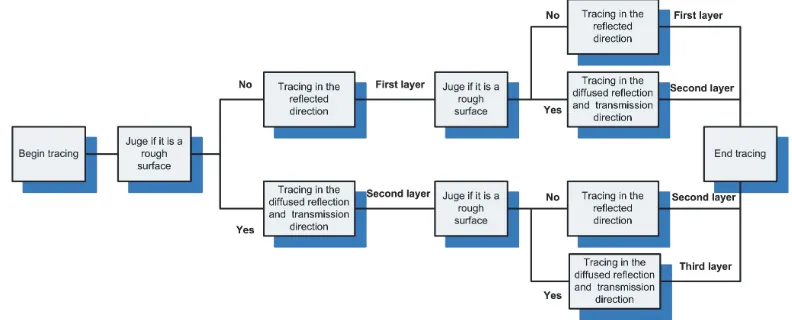
For the reason that the effect of diffused reflection and transmission should be considered in the simulation for rough surface imaging, all the rays have hierarchical structure in the tracing process. The hierarchical principal is detailed as follows. Rays which do not experience the diffused reflection or transmission are considered as the first layer, and those which experience once diffused reflection or transmission are considered as the second layer, and so on. Obviously, it can be discovered that the sensitivity of the brightness temperature is proportional to the layers. The schematic diagram is shown in Figure 1.
Figure 1. Schematic diagram of MBTT.
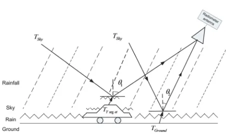
For the introduction of the MBTT principle, the physical model of space-to-ground scene is shown in Figure 2, in which a car is parked on the ground which is detected by the radiometer antenna in the space with rainfall background. The ground is covered by the rain. In the model, the top layer media is sky, the middle layer media is rain and the bottom layer is ground or the car. Two different cases are shown in the figure. One is the brightness temperature in the direction θ1, which is composed of the
sky, car, the rain and their coupling between each other. The other is the brightness temperature in the directionθ2, which is composed of sky, ground, the rain and their coupling. The brightness temperature
of the sky arrives at the antenna by the means of diffused reflection, while the brightness temperature of the car, the rain and the ground arrive at the antenna by the means of diffused transmission.
Figure 2. Physical model of car detecting in rain. Figure 3. Tracing model of MBTT of multi-layer medium rough surface.
is composed of three layers, the air, the rain and the ground. Two targets are located on the ground, which is covered by the rain. And the interface between the rain and the air is a rough one, while other interfaces in the model are smooth. After emitting, the ray crosses the rough surface after reflected by the target 1, and the cross point on the rough surface is set as a new source of a new layer to emit rays. The new rays can be divided into two classes according to the diffused reflection or transmission. Then the tracing will be terminated when the times of reflection and layer reach the certain number.
Assuming that the range of pitch angle is divided intoosegments, and azimuth angle ispsegments. In order to discriminate the different reflections and layers in the tracing, brightness temperature of each section is represented by Tij, the number of layer is expressed by i, if the number of maximum
layer is set as 3, then i = 1,3. The times of reflection is expressed by j, if the times of maximum reflection are set as 3, then j = 0,3. Therefore, the brightness temperature arrived at the radiometer is represented by T10(θo, ϕp) because it is the first layer, and the reflection time is 0. The brightness
temperature from the ground to target 1 is expressed by T11(θ2, ϕ2) because it has been reflected by
the target 1, and θ2 is the incident degree of the ray. The brightness temperature from the ground to
the cross point in the direction (θt, ϕt) is expressed by T20(θt, ϕt) because it is the second layer which
has not been reflected by any surface after emitted from the new source. The brightness temperature from the sky to the target 2 in direction (θ3, ϕ3) is expressed by T21(θ3, ϕ3).
2.2. Retrieving Model of Layered Media
The source in the tracing model is the radiometer antenna. For a real case, the source is the target or the sky, and the retrieving process is from the source to the radiometer. In the retrieving model, only the brightness temperature from the top layer is considered in the case of single layer, however the brightness temperature from the bottom layer is neglected, which is of practical important in the model of multilayer. Figure 4 shows the retrieving model of the MBTT of multi-layer surface scene.
As shown in Figure 4,T10(θo, ϕp) represents the brightness temperature arrived at the radiometer,
which is composed of the brightness temperature of the air in the incident direction Tup(θ2, ϕ2), the
brightness temperature from the target 1 T1·e1(θ1) and the brightness temperature from the rain that
reflected by target 1T11(θ2, ϕ2)·r1(θ2). It can be expressed by Equation (1).
T10(θo, ϕp) =T11(θ2, ϕ2)·r1(θ2) +T1·e1(θ2) +Tup(θ2, ϕ2) (1)
The brightness temperature from the ground arriving at target 1, T11(θ2, ϕ2), is composed of the
brightness temperature from the rain itself, coherent components and the non coherent components. It can be expressed by Equation (2).
T11(θ2, ϕ2) =
T12(θ1, ϕ1)·rp(θ1)·e(−4k
2s2cos2(θ1))
+T2tol(θ1, ϕ1) +TR·erp(θ1)
Figure 4. Retrieving model of the MBTT of multi-layer rough surface scene.
20 30 40 50 60 70 80
245 250 255 260 265 270 275 280 285
B
right
ne
s
s
t
e
m
p
e
ra
tur
e
(K
)
Zenith angle(degree) calculation result of grass (improving method) measured value of grass
calculation result of sand (improving method) measured value of sand
calculation result of sand (tradional method) calculation result of grass (tradional method)
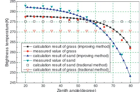
Figure 5. Comparison of the measured values.
In Equation (2), the first item is the coherent components, and the third item is the brightness temperature from the rain itself. TRis the average temperature of the rain, anderp(θ1) is the emissivity
of the rain in direction θ1.
For single layer, the second item in Equation (2), T2tal(θ1, ϕ1), is only the total brightness
temperature of the second layer after diffused reflection in direction (θ1, ϕ1), which can be expressed by
Equation (3).
T2tol(θ1, ϕ1) =
i=1,N
j=1,M
T20(θi, ϕj)·Γ(θi, ϕj;θ1, ϕ1). (3)
In Equation (3),T20(θi, ϕj) is the brightness temperature from arbitrary diffused reflection direction
arrived at the source of second layer. Γ(θi, ϕi;θ1, ϕ1) is the reflectivity from the direction (θi, ϕj) to the
direction (θ1, ϕ1).
For layered media, besides the diffused reflection, the diffused transmission should also be taken into consideration in the non-coherent components. Therefore, modified T2tal(θ1, ϕ1) in Equation (2)
will be expressed as Equation (4).
T2tol(θ1, ϕ1) =
i=1,N
j=1,M
T20(θi, ϕj)·Γ(θi, ϕj;θ1, ϕ1) +
k=1,N
l=1,M
T20(θk, ϕl)·Γt(θk, ϕl;θ1, ϕ1). (4)
In Equation (4), T20(θk, ϕl) is the brightness temperature from arbitrary diffused transmission
direction arrived at the source of second layer. Γt(θk, ϕl;θ1, ϕ1) is the transmittivity from the direction
(θk, ϕl) to the direction (θ1, ϕ1), which can be expressed by Equation (5).
Γpt(θk, ϕl;θ1, ϕ1) = θ1+2πN
θ1−2πN ϕ1+Mπ
ϕ1−Mπ
[σppt(θk, ϕl;θ1, ϕ1) +σpqt(θk, ϕl;θ1, ϕ1)]·sin(θ1)
4πcos(θk) dθ1dϕ1.
(5)
Γ(θi, ϕj;θ1, ϕ1) is the reflectivity from direction (θi, ϕj) to (θ1, ϕ1), which can be obtained in
Equation (6).
Γp(θi, ϕj;θ1, ϕ1) = θ1+2πN
θ1−2πN ϕ1+Mπ
ϕ1−Mπ
[σpp(θi, ϕj;θ1, ϕ1) +σpq(θi, ϕj;θ1, ϕ1)]·sin(θ1)
4πcos(θi) dθ1dϕ1.
(6)
In Figures 5 and 6, σppt(θk, ϕl;θ1, ϕ1) and σpp(θi, ϕj;θ1, ϕ1) are respectively the transmission and
reflection coefficient. The derivation of the two coefficients contained in [14]. In Figure 4,T20(θk, ϕl) is
taken as an example. It can be expressed by Equation (7).
where TD is the physical temperature of the ground, ed(θk) the emissivity of the ground in direction
θk, γ the attenuation coefficient of the rain, d the effective distance, and T21(θk, ϕl) the brightness
temperature from the rain surface down to the ground.
Besides the difference mentioned above, the emissivity of the rough surface in Equation (2) is also different from which in the case of single layer. For the case of single layer, we have
erp(θ1) = 1−rcorp(θ1)−rnonrp (θ1). (8)
For the case of multi-layer, the transmittivity of the rough surface should also be considered, and we have
erp(θ1) = 1−rrpco(θ1)−rrpnon(θ1)−trp(θ1), (9)
wheretrp(θ1) is the transmittivity from the rain to the air in directionθ1, and rrpnon(θ1) andtrp(θ1) are
expressed by Equations (10) and (11).
rrpnon(θ1) =
Ω
[σpp(θ1, ϕ1;θi, ϕj) +σpq(θ1, ϕ1;θi, ϕj)]·sin(θi)
4πcos(θ1) dθidϕj,
(10)
trp(θ1) =
Ω
[σppt(θ1, ϕ1;θk, ϕl) +σpqt(θ1, ϕ1;θk, ϕl)]·sin(θ1)
4πcos(θ1) dθkdϕl.
(11)
Then, we can obtain the modified brightness temperature from the rain to target 1 T11(θ2, ϕ2)
by combining Equations (4), (5), (6), (7), (9), (10) and (11) with (3). Thereafter, the brightness temperature arrived at the antenna, T10(θo, ϕp), can be obtained by Equation (1).
3. EXPERIMENTS AND ANALYSIS
3.1. Real Case of Grass and Sand
The proposed model is used to calculate the brightness temperatures of grass and sand for validation (Figure 5). Figure 6 shows the measured grass scene using a millimeter radiometer. The measurement is performed using a working frequency of 35 GHz, frequency bandwidth of the radiometer antenna of
Radiometer
Figure 6. Measured scene of the grass.
Buried Target
Radiometer
1 GHz, and distinguishability of 5.5◦. The root mean square height and correlation length of the grass are 3.5λand 10λ, respectively. And the root mean square height and correlation length of the sand are 3.0λand 13λ, respectively, which is smoother than the grass. The bottom layer of the grass and sand is soil. The complex permittivity values of the grass, sand, and soil are set as (1.353, 0.070), (5.1, 0.1), and (2.1, 0.9), respectively [15, 16].
As shown in Figure 5, for both media, the calculated values with the traditional method do not change with the zenith angle, because the Lambertian model is used in the traditional method which set the emissivity of the rough surface as a consistent value. The calculated values with the improved method are closer to the measured ones, but the slopes differ. The slope of the grass is lower than that of the sand possibly because of their different roughness levels. Hence, we conclude that the proposed model is accurate and feasible. To further study the effect of the proposed model, we perform simulation in 3D scene imaging.
3.2. Simulation in PMMW Imaging of Buried Targe
Figure 7 presents the optical image of targets buried in the sand. Some metal objects, which contain a six-face cylinder and a hexahedron, are selected as targets. Figure 8 shows the measured image by the radiometer, and Figure 9 demonstrates the model of the real scene.
In the scene of Figure 9, the depth of the sand is 0.25 m, the pitch angle ranges from 8◦ to 68◦, and the azimuth angle from −10◦ to +10◦. The root mean square height and correlation length of the sand are 3.0λand 13λ, respectively, and the complex permittivity of the targets is set as (3.5, 1.2). Figure 10 shows the simulated image of the scene.
-10 -8 -6 -4 -2 0 2 4 6 8 10 -30
-20 -10 0 10 20
30 194.0
195.8
197.6
199.5
201.3
203.1
204.9
206.7
208.5
210.4
212.2
214.0
Figure 8. Measured image of the real scene.
Figure 9. Model of the real scene.
-10 -8 -6 -4 -2 0 2 4 6 8 10 -30
-20 -10 0 10 20
30 192.0
194.0 196.0 198.0 200.0 202.0 204.0 206.0 208.0 210.0 212.0 214.0
The simulated results accurately reproduce the measured image of the radiometer. However, a slight difference exists between the measured and simulated images because of the scene modeling. We can conclude from the simulation of the buried target that the proposed multi-layer rough surface model is effective. To further study the characteristics of a multi-layer rough surface, we simulate a 3D virtue scene.
3.3. Simulations in PMMW of Virtue Scens
Figure 11 shows the virtue scene model. The pitch angle of the radiometer antenna ranges from 8◦to 68◦, and the azimuth angle ranges from−10◦ to +10◦. A hexahedron metal is located on the ground with a complex permittivity of (3.5, 1.2). The ground is assumed to be bail soil with a complex permittivity of (2.1, 0.45). The dry snow is located at 0.05 m depth on the ground and also the roof of the hexahedron. The complex permittivity of the dry snow varies depending on working frequency and moisture [17, 18]. For calculations, we set the working frequency as 10 GHz. Note that in the simulations of virtue scenes, environmental factors, such as fog and cloud cover, are not considered for the ambient temperature of the target [19–22].
To study the effect of surface roughness on the simulated image, we conduct calculations using the same model with different correlation lengths. Figures 12(a)–(d) show the simulated images. In the calculation, the average brightness temperature of the sky background, target, dry snow, and ground are assumed to be 180 K, 300 K, 220 K, and 300 K, respectively. The moisture of the dry snow is set as 12%, and the complex permittivity is (2.5, 0.9).
As shown in Figures 12(a)–(d), the four simulated images accurately reproduce the scene and are generally similar. The target buried in the dry snow can be detected by the radiometer. The brightness temperatures from various pitch angles as well as the ranges of which differ among the four images. However, when the pitch angle is the same, the brightness temperature is similar among different azimuth angles.
-10 -8 -6 -4 -2 0 2 4 6 8 10 -30
-20 -10 0 10 20
30 219.0
220.0 221.0 222.0 223.0 224.0 225.0 226.0 227.0 228.0
(a)
-10 -8 -6 -4 -2 0 2 4 6 8 10 -30
-20 -10 0 10 20 30
(b)
219.0
220.1
221.3
222.4
223.5
224.6 225.8
226.9
228.0
-10 -8 -6 -4 -2 0 2 4 6 8 10 -30
-20 -10 0 10 20
30 219.0
219.5 220.0 220.5 221.0 221.5 222.0 222.5 223.0 223.5 224.0
(c)
-10 -8 -6 -4 -2 0 2 4 6 8 10 -30
-20 -10 0 10 20
30 219.4
219.6 219.8 220.1 220.3 220.5 220.7 220.9 221.2 221.4 221.6
(d)
To observe changes in the brightness temperature with different pitch angles of each roughness value, we construct four curves with an azimuth angle of −8◦ (Figure 13). This study is based on the fact that the brightness temperature is related to pitch angle, but not to azimuth angle. The pitch angle is represented by θi in the follow figures.
In Figure 13, the four curves represent four different correlation lengths. The range of the brightness temperature decreases with increasing correlation length. This change is in contrast to that in single layers. Figure 14 shows the change curves of single-layer grass.
Changes in the brightness temperature decrease with increasing correlation length. The brightness temperature from the bottom layer differs between single and multiple layers. For the multi-layer, the brightness temperature arrived at the radiometer includes temperatures from diffuse air reflected by the rough surface, temperature from the surface itself, and temperature from the bottom layer. However, in the single layer, the brightness temperature is obtained from the top layer only. Figure 15 shows the change curves of brightness temperature from the bottom layer.
As shown in Figure 15, the change curves of the brightness temperature from the bottom layer are the same as the brightness temperature arrived at the radiometer. The brightness temperature reflected by the surface is lower than that from the bottom layer. The brightness temperature from the bottom layer determines the change curves. As such, we perform calculations with the same model
0 10 20 30 40 50 60 70
218 220 222 224 226 228 230 B rig h tn e s s t e m p er at u re( K )
θi(degree)
L=10λ L=15λ L=20λ L=25λ
σ=1.5λ
Figure 13. Change curves of brightness tem-perature with pitch angles of different correlation lengths.
30 40 50 60 70
150 160 170 180 190 200 B right ne s s t e m p e ra tur e (K )
θi(degree) L=6λ L=8λ L=10λ L=12λ L=15λ L=20λ
Figure 14. Change curves of brightness tem-perature with pitch angle of different correlation lengths of single layer.
0 10 20 30 40 50 60 70
28 30 32 34 36 38 40
θi(degree)
B rig ht ne s s t e m p e ra tur e (K
) L=10 L=15λλ
L=20λ L=25λ
using different root mean square (RMS) heights. Figures 16(a)–(d) show the simulated images. The other parameters are set the same as those in Figure 12.
In Figures 16(a)–(d), the four simulated images accurately reproduce the scene. The brightness temperatures from various pitch angles as well as the ranges differ among the four images. However, for a uniform pitch angle, the brightness temperature remains the same for different azimuth angles.
To observe the brightness temperature changes with pitch angles of varying roughness levels, we construct four curves with an azimuth angle of −8◦ (Figure 17).
-10 -8 -6 -4 -2 0 2 4 6 8 10 -30 -20 -10 0 10 20 30 219.0 220.0 221.0 222.0 223.0 224.0 225.0 226.0 227.0 228.0
-10 -8 -6 -4 -2 0 2 4 6 8 10 -30 -20 -10 0 10 20 30 218.0 219.0 220.0 221.0 222.0 223.0 224.0 225.0 226.0 227.0 228.0 229.0 230.0
-10 -8 -6 -4 -2 0 2 4 6 8 10 -30 -20 -10 0 10 20 30 216.0 217.0 218.0 219.0 220.0 221.0 222.0 223.0 224.0 225.0 226.0 227.0 228.0 229.0
-10 -8 -6 -4 -2 0 2 4 6 8 10 -30 -20 -10 0 10 20 30 216.0 217.0 218.0 219.0 220.0 221.0 222.0 223.0 224.0 225.0 226.0 227.0 (a) (b) (c) (d)
Figure 16. Simulated images with different roughness levels. In the four images, the RMS is set as
L= 10λ. (a)σ= 1.0λ, (b) σ= 1.5λ, (c)σ = 2.0λ, and (d) σ= 2.5λ.
0 10 20 30 40 50 60 70
215 216 217 218 219 220 221 222 223 224 225 226 227 228 229 σ=λ σ=1.5λ σ=2.0λ σ=2.5λ B right ne s s t e m p e ra tur e (K )
θi(degree)
L=10λ
Figure 17 shows that the change range of the brightness temperature increases with increasing RMS height. The higher the RMS height is, the deeper the roughness is. Therefore, the change range of the brightness temperature is proportional to the roughness in the same medium. To determine the effect of complex permittivity on brightness temperature, we simulate images of dry snow with different moisture contents, while keeping RMS height and correlation length the same (Figures 18(a)–(d)).
In Figures 18(a)–(d), the complex permittivity is set as (2.5, 0.9), (2.3, 0.7), (2.0, 0.5), and (1.6, 0.2) for (a), (b), (c), and (d), respectively [17]. The change range of the brightness temperature differs among the four images and is difficult to discriminate in Figure 18. To observe the brightness temperature changes with pitch angle and moisture, we construct four curves at an azimuth angle of−8◦(Figure 19). Figure 19 shows that the changes in the brightness temperature with different complex permittivity values are smaller than the changes with roughness; the range of the brightness temperature increases with increasing moisture content of the dry snow. However, the sharpness of the curves at varying moisture contents remains almost the same. To determine the effect of the thickness of the dry snow on the brightness temperature, we construct three curves of brightness temperature with pitch angles of varying thicknesses (Figure 20).
In Figure 20, the RMS height and correlation length are set as 1.5λand 10λ, respectively. And the moisture content of the dry snow is set as 12%. The curves vary with thickness. When the thickness of the dry snow is 0.02 m, the curve sharpness is the same as that shown in Figure 13. When the thickness is 0.08 m; the sharpness is closer to the curve of the single layer. When the thickness is 0.2 m, the sharp of the curve is similar to that of the single layer (Figure 14). Hence, the effect of the brightness temperature from the bottom layer decreases with increasing thickness. When the thickness is sufficiently deep, the effect of the bottom layer should not be considered in the calculation. This conclusion conforms to physical laws, thereby confirming the correctness of the model and method used in this paper.
-10 -8 -6 -4 -2 0 2 4 6 8 10 -30
-20 -10 0 10 20
30 219.0
220.0 221.0 222.0 223.0 224.0 225.0 226.0 227.0 228.0
(a)
-10 -8 -6 -4 -2 0 2 4 6 8 10 -30
-20 -10 0 10 20 30
(b)
219.0 220.0 221.0 222.0 223.0 224.0 225.0 226.0 227.0 228.0
-10 -8 -6 -4 -2 0 2 4 6 8 10 -30
-20 -10 0 10 20 30
(c)
219.0 220.0 221.0 222.0 223.0 224.0 225.0 226.0 227.0 228.0
-10 -8 -6 -4 -2 0 2 4 6 8 10 -30
-20 -10 0 10 20 30
(d)
219.0
220.0
221.0
222.0
223.0
224.0
225.0
226.0
227.0
0 10 20 30 40 50 60 70 218
220 222 224 226 228
B
right
ne
s
s
t
e
m
p
e
ra
tur
e
(K
)
θi(degree) 12%
10% 8% 6%
L=10λ σ=1.0λ
Figure 19. Change curves of brightness temper-ature with pitch angles of different moisture con-tents in the dry snow.
0 10 20 30 40 50 60 70
200 205 210 215 220 225 230
d=20cm d=8cm d=2cm
B
rig
h
tn
e
s
s
t
e
m
p
er
at
u
re(
K
)
θi(degree)
Figure 20. Change curves of brightness temper-ature with pitch angle of different thicknesses in the dry snow.
4. CONCLUSION
This paper proposes an improved model for simulation of a scene with multi-layer rough surface in PMMW imaging. MBTT considers diffused transmission from the bottom layer. The improved model is correct and effective for simulating multi-layer rough surfaces. The applicable range of the brightness temperature tracing method is extended, and the scene with buried target can be simulated by the method.
The effects of different RMS height, correlation length, and roughness of the dielectric constant of the rough surface are studied and analyzed. For the same material, RMS height is proportional to radiation brightness temperature, and correlation length is inversely proportional to radiation brightness temperature. Thus, roughness is proportional to brightness temperature in the same medium. Increases in RMS height and decreases in correlative length both indicate increases in roughness. The curve of the multi-layer is determined by the brightness temperature from the bottom layer. The results reveal that changes of brightness temperature with different complex permittivity values are less than the changes with different roughnesses. Finally, different thicknesses of the bottom layer are simulated. The effect of the brightness temperature from the bottom layer decreases with increasing thickness but should not be considered in the calculation when the thickness is sufficiently high.
ACKNOWLEDGMENT
This work is supported by the National Natural Science Foundation of China State Key Laboratory of Millimeter Waves, Natural Science Foundation of Jiangsu Province and Specialized Research Fund for the Doctoral Program of Higher Education under grant numbers 61071021, K201413, BK2012435 and 20133223120005, respectively.
REFERENCES
1. Liu, G. D. and Y. R. Zhang, “Three-dimensional microwave-induced thermo-acoustic imaging for breast cancer detection,” Acta Phys. Sin., Vol. 60, No. 7, 074303, 2011.
3. Zhang, X., H. Tortel, S. Ruy, et al., “Microwave imaging of soil water diffusion using the linear sampling method,”IEEE Geoscience & Remote Sensing Letters, Vol. 8, No. 3, 421–425, 2011. 4. Ruf, C. S., C. T. Swift, A. B. Tanner, et al., “Interferometric synthetic aperture microwave
radiometry for the remote sensing of the Earth,” IEEE Transactions on Geoscience & Remote Sensing, Vol. 26, No. 5, 597–611, 1988.
5. Yujiri, L., M. Shoucri, and P. Moffa, “Passive millimeter wave imaging,” IEEE Microwave Magazine, Vol. 4, 39–50, 2003.
6. Salmon, N. A., R. Appleby, and S. Price, “Scene simulation of passive millimeter-wave images of plastic and metal objects,” Proc. SPIE, 397–401, 2002.
7. Salmon, N. A., “Polarimetric scene simulation in millimeter-wave radiometric imaging,” Proc. SPIE, 260–269, 2004.
8. Salmon, N. A., “Polarimetric passive millimeter-wave imaging scene simulation including multiple reflections of subjects and their backgrounds,” Proc. SPIE, 354–358, 2005.
9. Zhang, C. and J. Wu, “Near-field 3D scene simulation for passive microwave imaging,”Proc. SPIE, Vol. 6419, 1–11, 2006.
10. Zhang C. and J. Wu, “Image simulation for ground objects microwave radiation,” Journal of Electronics &Information Technology, Vol. 29, 2725–2728, 2007.
11. Fetterman, M. R., J. Dougherty, and W. L. Kiser, Jr., “Scene simulation of mm-wave images,” IEEE 2007 AP-S Int. Symposium, 1493–1496, 2007.
12. Fetterman, M. R., J. Grata, and G. Jubic, “Simulation, acquisition and analysis of passive millimeter-wave images in remote sensing applications,” Optics Express, Vol. 25, 20503–20515, 2008.
13. Salmon, N. A., “Scattering in polarimetric millimetre-wave imaging scene simulation,”Proc. SPIE, Vol. 6211, 71–78, 2006.
14. Fawwaz, T., R. Ulaby, K, Moore, and K. F. Adrian,Microwave Remote Sensing Active and Passive, 1982.
15. Zhang J. R., D. H. Zhang, L. W. Wang, Y. Z. Zhao, W. Sheng, and W. Guo, “In situ measurement of typical objects’ permittivities in microwave remote sensing,”Journal of Electronics, Vol. 4, 566-9, 1997.
16. Zhang, J. R., “The microwave dielectric constant of canopy and soil,”Remote Sensing Technology and Application, Vol. 10, 40–50, 1995.
17. Sun, Z. W., P. S. Yu, and L. Xia, “Progress in study of snow parameter inversion by passive microwave remote sensing,”Remote Sensing for Land & Resources, Vol. 27, No. 1, 9–15, 2015. 18. Jiang, L. M., J. C. Shi, and L. X. Zhang, “Comparison of dry snow emission model with
experimental measurements,”Journal of Remote Sensing, Vol. 10, No. 4, 515–522, 2006.
19. Liebe, H. J., G. A. Hufford, and M. G. Cotton, “Propagation modeling of moist air and suspended water/ice particles at frequencies below 1000 GHz,” Atmospheric Propagation Effects Through Natural and Man-Made Obscurants for Visible to MM-Wave Radiation, Vol. 11, SEE N94-30495, 08–32, 1993.