Fast Ray Simulation Method Applied in Microwave Radiation Brightness Temperature Imaging

Fast Ray Simulation Method Applied in Microwave

Radiation Brightness Temperature Imaging

Chuan Yin

_,

_{Ju Qian}

_{, Ming Zhang}

_{, Yaming Bo}

1 _{School of Electronic Science and Engineering ,Nanjing University of Posts and Telecommunications, Nanjing} 210003, China.

2 _{State Key Laboratory of Millimeter Waves, Southeast University, Nanjing 210096, China.}

*Corresponding author. Tel.: 025-85866131; email: [email protected]

Manuscript submitted March 25, 2016; revised July 20, 2016.

doi: 10.17706/jcp.12.6.486-499

Abstract: Large-scale simulation and high quality of microwave brightness temperature imaging is the key technology for passive target detection. We applied the space meshing ray tracing method for brightness temperature tracing to establish a model of tracing and inversion. Simulated images were then compared with the measured images to verify the effectiveness of the proposed method. Results showed that the space meshing ray tracing method can significantly improve the calculation efficiency, thereby allowing high-accuracy large-scale simulation using the same calculation. The effect of the low-pass filter on the simulated image was also considered.

Keywords: Radiation brightness temperature, simulation in microwave imaging, space meshing ray tracing,

high accuracy.

1.

Introduction

Microwave imaging has attracted considerable interests in recent years because of its ability to penetrate the atmosphere, cloud and mist, dust, and so on [1]-[5]. Passive microwave imaging is widely used because of stealth detection and target discrimination [6]-[8].

Passive microwave imaging was first applied in remote sensing in 1960s [9]. Then, the advanced large-scale instantaneous imaging technology was developed in the late 90s [10], [11], which led to the development of simulation techniques for passive microwave imaging.

Image simulation of passive microwave radiation for the study of various targets is important. Radiation characteristics through simulation can aid in the understanding of the goal, explaining some radiation phenomenon, identifying specific radiation law, and determining whether the actual measurement result is good or bad. Various factors affecting radiometer system design, such as working environment, operating frequency, antenna size, observing distance, and image processing algorithms, must be considered for an effective image simulation in different environmental conditions. For convenient application and quick assessment, an image can be simulated on the basis of radiation gauge properties, which could serve as an effective complement or alternative to field measurements. This method of image simulation could save valuable time, money, manpower, and material resources.

to count the coupling. The later method is flexible and is adjustable within a certain range of image resolution.

The two aforementioned approaches can be both utilized, however, they both need the small plane intersection test in the simulation, and the order of the calculation growth is relatively large. Therefore, developing a fast and highly efficient simulation of large-scale complex environment imaging is difficult because of the nature of the calculation. To simulate a large-scale complex scene, we proposed a highly efficient imaging method using fast ray tracing technology.

Space meshing ray tracing method [17], [18] is based on the meshing division of the tracing space, and uses the relationship of the meshing to realize fast ray tracing. The key idea of the said method is to divide the space model into several simple joint geometric grid units. Then, the geometrical relationship between the ray propagation path and the grid cell will be used to calculate the ray propagation path. Hence, in the same amount of calculation, intersection test can be avoided to achieve fast calculation and highly accurate analysis of the dense ray. In this paper, the authors applied the space meshing ray tracing method to the brightness temperature tracing method. Results revealed that the method can efficiently simulate the sophisticated scene precisely and accurately. The two-dimensional analysis model of radiant brightness temperature was established in Section 3. In Section 4, the correctness of the improved method was verified by comparing the measurement of the simulated image of a plane’s runway with the actual runway measurement. We also simulated a three-dimensional virtual image of the scene to study the effect of microwave imaging simulation on ray interval. Another image was simulated to verify the effect of the low-pass filter. Finally, the authors compared the results of the improved method with the traditional one to demonstrate the high efficiency of the improved approach.

2.

Physical Model

The physical model of passive radiation included the radiation from targets, the atmosphere, the sun and the reflection between targets. The radiometer was placed in a certain position to receive the synthesized brightness temperature.

2.1.

Radiation from Targets

The electromagnetic wave was radiated from any object whose temperature was above zero. When an object is in a state of heat balance, the energy radiated outward is equal to the energy absorbed. The ideal complete absorber is called a "black body", and the relationship between its thermal radiation spectrum brightness, temperature, and wavelength can satisfy Planck’s black body radiation law [9].

3 2

5

2 1 2 1

( ) ( )

1 1

f hf kT hf kT

hf hc

B

c e



 

  (1)

For the above equation, Bf is the black body’s spectrum brightness, whose unit is

2 1 1

W m  sr Hz , his

the Planck’s constant ( 34

6.63 10  J), kis the Boltzmann constant (1.38 10 23J K 1), is the wavelength,

Tis the absolute temperature, f is the frequency, whose unit isHz, and c is the velocity of light.

For millimeter wave band, equation (1) can be simplified into approximate expressions (2) by Rayleigh Jeans given thathf kT1.

2

2

f

B T

k 



(2)

physical bodies are gray in nature, and their transmission power is generally less than the black body. The brightness temperature of gray is defined asB( , )  when its temperature isT. In the same temperature, the emissivity can be defined as the ratio of brightness of gray to black body, which is represented by  ( , ).

In general, the emissivity of the object is determined by the dielectric constant, roughness, physical temperature, direction, wavelength, polarization, and so on. The object surface can be divided into four categories according to the degree of roughness, which includes the following: smooth surface (ks0.1),

micro rough surface (0.1ks0.3), medium rough surface (0.3ks1), and extremely rough surface

(ks1). In the actual scene, many artificial objects can be considered having a smooth surface, such as

vehicles, roads, buildings, and so on, whereas most natural objects are classified as rough surfaces, such as the earth, the vegetation, the ocean, and so on.

2.2.

Radiation from the Atmosphere

Aside from the targets, the model of microwave radiation also includes radiation from the atmosphere. On condition that the atmospheric scattering is neglected, the downward and upward atmospheric radiation brightness temperatures can be expressed by:

' ) ' ( ) ' ( sec ) ,

( (0,')sec

0 dz e z T z k T z H a UP      



( (0, ')sec

dz e z T z k T z H a DN       



where, is the zenith angle, k_a( ')z is the absorption coefficient of the atmosphere when the height isz',

( ')

a

T z is the temperature of the atmosphere, and (0, ')z is the optical depth in the vertical direction between 0 and z', which is defined in (5) as:

' ) ' ( ) ' , 0 ( ' 0 dz z k z z a



2.3.

Brightness Temperature Output of Antenna

In the radiation measurement, the brightness temperature of the antenna mouth is not the measured value. The effect of the radiometer on the brightness temperature should be considered to calculate the real measured value. According to the measurement principle, the relationship between the calibration output brightness temperature of the antenna and the antenna mouth can be expressed by (6) as:





where, TAP is the brightness temperature of the in- mouth antenna, TA is the output brightness

temperature of the antenna, and Fnis the weighting result of antenna pattern. The weighting has a smooth

effect on the input brightness temperature of the antenna; therefore, the weighted image will have a gradient area at the edge of the target and background. The ideal normalized power pattern of the uniform distribution circular aperture antenna can be expressed by (7) as:

2 2 1 2 cos 1 / sin ) / sin ( 2 ) , (            



















width is3dB D, and the resolution of the imaging system is determined by the power direction of the

antenna.

2.4.

Effect of the Receiver

The brightness temperature output from the radiometer is not only affected by the antenna but is also influenced by the receiver. The low-pass filter in the receiver is considered as an integrator, which affects the brightness temperature output of the antenna. Given that is the integral time, the output voltage from the antenna isV t( ), and the output voltage from the low-pass filter isVout( )t , we obtain the equation:

0

( ) ( ) ( )

t out

V t 



(8)

1 / 0

( )

0 0

t h t     

 (9)

By combining the convolution formula with (8), we obtain the equation:

( ) ( ) ( ) out

V t h t v t

(10)

Based on (10), the brightness temperature output from the receiver is the convolution of the brightness temperature output from the antenna and the stimulating signalh t( ).

3.

Brightness Temperature Tracing

The fundamental idea of the brightness temperature tracing is to simulate the radiometer scanning. Each scan can be regarded as a ray, which will experience many physical processes, such as multiple reflections, collision and penetration, in the propagation path. After the whole physical process, the radiation brightness temperature arriving in the radiometer is retrieved. Aside from field intensity ray tracing, the brightness temperature in different directions is independent and has no path attenuation in the clear sky.

3.1.

Modeling of Brightness Temperature Retrieval

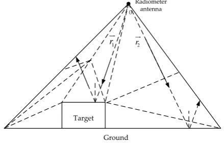
In practice, the targets are mostly non-transparent objects; therefore, the transmission is insignificant. More than one reflection time will cause another radiation source level; the atmospheric radiation is regarded as the source if the ray is emitted into the air. For simplicity, we assumed that the brightness temperature is only related to the angle of pitch. Based on this assumption, a two-dimensional model of detecting targets on the ground was established. The retrieval process is shown in Fig. 1.

D T 1  2  O T 2 ( ) B T  ) (2 UP

T

) (1 DN T Rad iom ete_r ant enna ) (1 DUP T 3 ( ) B T  3  3 ( ) DN T  3 ( ) UP T  4  4 ( ) DN T  4 ( ) UP T  4 ( ) B T 

In Fig. 1, three different cases are shown, the radiation from the atmosphere down to the ground or targets, which are calledT_DN( )₁ , T_DN(₃)and T_DN(₄)serve as the sources. T_Ddenotes the absolute temperature of the ground, the emissivity of the ground in the direction₁is represented by _D( )₁ , whereas

O

T denotes the absolute temperature of target, and  _O( ₂)and _O( ₃)denote emissivity of the target in

direction₂and₃.The brightness temperature,T_B(₂), is composed of two parts, which are from the

atmosphere TUP(2)and the target, when the effect of the radiometer is ignored. The brightness

temperature of the target, which comes from the groundTDUP( )1 , is also made up of two parts: the target

itself and the brightness temperature reflected by the target.TB(2)is given by (11) as:

2 2 2 1 2

( ) ( ) ( ) ( )(1 ( ))

B UP o o DUP o

T  T  T  T   

(11)

When TDUP( )1 is the brightness temperature arriving at the target, we use the equation:

)) ( 1 )( ( ) ( )

(1 DD 1 DN 1 D1

DUP T T

T   

(12)

We combine equations (11) and (12) to obtainTB(2)to determine the brightness temperature arriving at

the antenna.TB(2)is also composed of two parts, TUP(2)and the target, which is given by (13).

3 3 3 3 3

( ) ( ) ( ) ( )(1 ( ))

B UP o o DN o

T  T  T  T   

(13)

In the actual scene, all the variables are not only related to the pitch angle  _{and azimuth angle} .

3.2.

Modeling of Ray Tracing

Ray tracing is a technology used in predicting the radio wave propagation characteristics in indoor and outdoor environment. This technology is based on the principle of geometrical optics, geometrical diffraction, and uniform wedge diffraction. The direct reflection and diffraction propagation mechanisms were considered in ray tracing. Thus, ray tracing is now widely used in various fields [19]-[22].

Traditional ray tracing is used to approximate the surface of the target using small planes. The interface test between ray and plane is needed in tracing. The calculation of intersection test is not only related to the number of rays, but also to the times of reflections. However, the test can be ignored in space meshing ray tracing method, in which the reflection points of the rays are found directly by using the adjacency relationship between the tetrahedral meshing and the scene.

In this paper, we used the triangle as the mesh unit. After meshing, the tracing space was divided into several seamless joint tetrahedrons. All triangular faces in the scene are composed of two kinds: the one that is already present in the model is called the real face, and the other kind is called the virtual face because of the meshing. After initial tracing, the ray will meet some faces in the tracing path. If the face is a virtual one, the ray will pass through the face and continue tracing. However, if the face is real, the ray will trace in the reflection direction after being reflected by the face. Thus, tracing will terminate once the reflection times reach the set value or the ray goes out of the space. The idea of tracing is shown in Fig. 3, where the interface is represented by line segments, the dotted lines indicate the virtual faces, and solid lines indicate the real faces.

closed environment, the shape of the meshing space is modeled according to the shape of the environment. As a result, the environment outside the meshing space should also be involved in modeling and analysis.

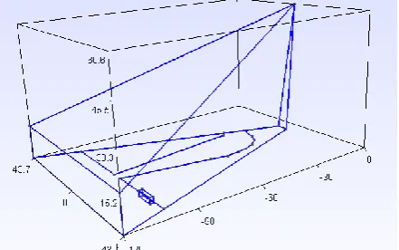
The model of detecting the target on the ground is established by the principle discussed above, and is revealed in Fig. 2. In a two-dimensional environment, the azimuth angle of the radiometer is not taken into account. According to the range of the pitch angle, a large triangle can be obtained, whereas several smaller triangles are obtained after meshing. Two rays escape the meshing space after being reflected by the target or the ground.

O

Ground Target

Radiometer antenna

1

r r2

Fig. 2. Two dimension model of space meshing ray tracing.

During tracing, the most critical problem is to trace the propagation path, which means judging the side from where the ray will come out of the known triangle. To address this problem, we used the extension coefficient method. When a ray crosses a triangle, the other two sides can be considered as possible edges. Then, the ray will be extended forward and backward, thus, the extended ray must intersect with the two possible edges at two cross points. Afterwards, two extension coefficients will be obtained. A positive extension coefficient indicates that the cross point is on the forward direction, whereas the backward direction is observed on a negative coefficient. The side with the smaller positive extension coefficient that the ray traverses through is the real edge. Afterwards, tracing will continue or terminate according to the principle stated above. The brightness temperature retrieval will begin when the tracing ends. If the meshing space is extended to three dimensions, the method discussed above will also be applicable on the condition that the triangle changes into tetrahedral, and the edge into a surface.

4.

Experiment and Imaging Results

4.1.

Simulated Image of Plane Runway

Fig. 3. Optical image of the runway. Fig. 4. Measured image of the runway.

using microwave imaging. Fig. 3 shows the optical image of the plane runway, while the measured image is revealed in Fig. 4. Cassegrain antenna with an aperture of 1.2 m and work frequency of 94 GHz was used as a radiometer. Fig. 5 shows the model of the plane runway. The grass next to the runway is an extremely rough surface, and its emissivity was approximated to a fixed value from arbitrary observing angles on the basis of Lambert’s approximate law, which was set at 0.85, and its brightness temperature as 270 K. the emissivity of the forest was set at 0.95, and its brightness temperature as 270 K. The simulated image is shown in Fig. 6.

Fig. 5. Model of the plane runway, in which the direction of the radiometer is defined by sphere angles

38o

  ,  0o _;  _{is the pitch angle of 60°,  is the azimuth angle, which is set as 20°,}

Runway

eps =6.0-j0.1,e_Grass =0.85,epsWarehouse=3.4-j0.02,TRunway=300K,TGrass=270K,TWarehouse =300K, TSky =180K,and

the ray interval is set as 0.1°.

-20 -15 -10 -5 0 5 10 15 20

-30 -20 -10 0 10 20

30 _180.0

190.0

200.0

210.0

220.0

230.0

240.0

250.0

260.0

270.0

280.0

290.0

Fig. 6. Simulated image of plane runway in vertical polarization.

As shown in Fig. 6, the simulation performed well in the imaging of the plane runway. However, the insignificant difference between the simulated image and the measured image is due to the difference in modeling. The results indicated that the brightness temperature of the runway monotonically decreased as the distance was decreasing. This decrease is because of the observe angle and the reflection of the sky. Moreover, the brightness temperature of the remote warehouses was lowest because the top of the warehouse is a metal material, thus, reflectivity is larger than its emissivity. In addition, due to its extremely rough texture, the brightness temperature of the grass next to the runway is constant and is independent with the incident angle and position. The black at the top of the image can be explained by the relatively low brightness temperature of the sky.

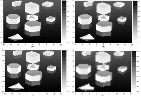
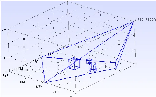
To discuss the effectiveness of the improved approach, we simulated the image of the three-dimensional virtual scene in this paper. As shown in Fig. 7, the work frequency of the radiometer was 90 GHz, which contains six hexahedrons of different sizes, a sphere, two six-sided cylinders, and a tetrahedral in different positions. They are all located on plane x-o-y, and the radiometer located at the vertex detects the targets, whose direction is defined by spherical angles 45o_and

45o

 ; the origin of coordinates is at the bottom of the ball. However, the diffraction and transmission are not considered in the model. Moreover, we assumed that the ambient temperature is not affected by environmental factors, such as rainfall, fog, and cloud cover [23]-[26].

Fig. 7. Three-dimensional model of Sceneepscube=epscylinder=3.4-j0.02,epssphere=epstetrahedral=8.0-j0.02,epsbottom surface=

6.0-j0.1,TSky=50K,TGround=250K,TTargets.=300K.Assuming that the range of the radiometer in the pitch angle and

the azimuth angle is 40°, and the meshing space is a four-sided cone.

-20 -15 -10 -5 0 5 10 15 20

-20 -15 -10 -5 0 5 10 15

20 220.0

230.0

240.0

250.0

260.0

270.0

280.0

290.0

300.0

(a) -20 -15 -10 -5 0 5 10 15 20

-20 -15 -10 -5 0 5 10 15

20 220.0

230.0

240.0

250.0

260.0

270.0

280.0

290.0

300.0

(b)

-20 -15 -10 -5 0 5 10 15 20

-20 -15 -10 -5 0 5 10 15 20

(c)

220.0

230.0

240.0

250.0

260.0

270.0

280.0

290.0

300.0

-20 -15 -10 -5 0 5 10 15 20

-20 -15 -10 -5 0 5 10 15 20

(d)

220.0

230.0

240.0

250.0

260.0

270.0

280.0

290.0

300.0

To determine the effect of ray interval of the simulation on microwave imaging, different angles of ray interval are set. The images of vertical polarized brightness temperature are revealed in Figures 8 (a-d). Moreover, considerable effort has been made to demonstrate that three levels are enough to simulate the radiation brightness temperature of the scene.

The four simulated images reproduced the scene well and are generally similar. However, the image was clearer when the ray interval is at 0.05°, the image of 0.1° was slightly obscure, and at 0.2°, a fuzzy wave shape appeared at the edge of the object and background. Moreover, the shape of the target began to blur when the ray interval was at 1°. As a result, the quality was enhanced with the decrease of the ray interval, thus, improving the simulation effect. The effect of the ray interval as a result of the method will be more evident in the simulation at long distances.

-20 -15 -10 -5 0 5 10 15 20

-20 -15 -10 -5 0 5 10 15 20

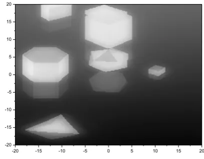
Fig. 9. Simulated image including the convolution effect of the low-pass filter.

To discuss the effect of the low-pass filter to the simulated image with ray interval at 0.2°, the effect of the convolution was considered as shown in Fig. 9. We also simulated the image without considering the effect of the convolution as shown in Fig. 10. The two images were almost similar, however, the focus on the edge were different. As shown in Fig. 10, the edge between the targets and the background was clearly seen, whereas in Fig. 9, the edge was blurred. Thus, the low-pass filter can provide a smooth image, similar to the effect of antenna on the image. Fig. 11 shows the simulated image, which included the effect of the antenna. Compared with Figs. 9 and 10, the edge between targets and the background was more blurred, and the image became smoother.

-20 -15 -10 -5 0 5 10 15 20

-20 -15 -10 -5 0 5 10 15 20

Fig. 10. Original simulated image.

-20 -15 -10 -5 0 5 10 15 20

-20 -15 -10 -5 0 5 10 15 20

4.3.

Comparison of Brightness Temperature Tracing

In the traditional approach of brightness temperature tracing, interface test is conducted on every small plane. Hence, the complexity of the model and the tested surface will double as the scale is incremented; the amount of calculation will also increase. Moreover, high distinguishability will further increase the amount of calculation. Thus, the shape of the target cannot be discriminated if the quality of the image does not meet the requirement.

To demonstrate the high efficiency of the improved method compared with the traditional method, we used both methods to simulate the same model. The model is shown in Fig. 12. In the open environment, the field expansion increases the complexity of the scene, thus, the number of targets that need to be detected also increases. Each of the detected objects is surrounded by the planes of different numbers. The planes and the sides of the scene denote the number of targets, which is considered as the variable of the model. Therefore, as shown in Fig. 12, the number of targets was 22, and if one more hexahedrons was added into the model, the targets will increase to 27. Different models with different numbers of targets were calculated to compare the efficiency of the two methods. The results are shown in Figs. 13–15.

Fig. 12. The model used to compare the two methods. In the model, the pentahedron has four targets, the hexahedrons have six targets, and the six-sided cylinders has seven targets. Four targets are coincident;

therefore, this model has 22 targets.

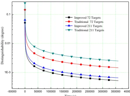
Fig. 13 shows the comparison of the two methods when the scale was increased in different ray intervals. The result indicated that the calculation time of the traditional brightness temperature tracing almost linearly increases. Moreover, different ray intervals have various slopes, which are proportional to the calculation time. On the other hand, shorter time was spent using the space meshing brightness temperature tracing approach. Fig. 14 illustrates the relationship between the scale and the calculation time in different ray intervals. In the same ray interval, the scale in which the improved method can detect was larger compared with the traditional method. The scale linearly increases, and the distinguishability is inversely proportional to the slope.

calculation, and enhance the image quality, thus meeting the demand of large-scale and high-quality imaging.

0 50 100 150 200 250

0 200 400 600 800 1000

Ti

me(s

)

Targets Improved 0.05degree Traditional0.05degree Improved 0.1degree Traditional0.1degree

Fig. 13. Comparison of the calculation time with the increase in the number of targets. Different models with different numbers of targets are calculated. Different curves show the different distinguishability with

different methods.

0 50 100 150 200 250 300

0 1000 2000 3000 4000 5000 6000

Ta

rg

et

s

Time (s)

Traditional 0.05degree Improved 0.05degree Traditional 0.1degree Improved 0.1degree

Fig. 14. Comparison of the targets when the calculation time is increased. The curves show different ray intervals with different methods, we can compare the scale that the two methods can detect in the same time.

-50000 0 50000 100000 150000 200000 250000 300000 350000 400000 1E-3

0.01 0.1

D

ist

in

g

u

ish

ab

il

it

y

(

d

eg

ree

)

Time (s)

Improved 72 Targets Traditional 72 Targets Improved 211 Targets Traditional 211 Targets

Fig. 15. Comparison of the distinguishability with the increase of calculation time, two different models with the different numbers of targets, 72 and 211 targets, respectively, are calculated, distinguishability of two

5.

Conclusion

In this study, space meshing ray tracing method for brightness temperature tracing was applied for the large-scale simulation in passive brightness temperature imaging with high accuracy. The model of brightness temperature tracing and retrieval was also established. The tracing process was described in detail to understand the improved method. Results indicated that the large-scale simulation with high distinguishability was efficiently realized by applying the proposed method. The correctness was verified by comparing the resulting image with the original measured image. The significance of ray interval to the simulation was demonstrated by comparing various images with different ray intervals.

The effect of the low-pass filter on the simulated image was discussed. Results showed that the low-pass filter can provide a smooth image; however, the edge between the targets and the background became blurry.

Furthermore, the high efficiency of the proposed method was verified by comparing the results with the original brightness temperature tracing method. The result indicated that the space meshing method for brightness temperature tracing can decrease the number of computation, and thus shorten calculation time, and enhance the image quality. However, the improved method is not sufficient in treating different rough surfaces. In addition, the diffusion reflection of rough surfaces was not considered. Further studies will be conducted to address these limitations.

Acknowledgments

This work is supported by the National Natural Science Foundation of China State Key Laboratory of Millimeter Waves, Natural Science Foundation of Jiangsu Province and Specialized Research Fund for the Doctoral Program of Higher Education under grant numbers 61071021, K201413, BK2012435 and 20133223120005, respectively.

References

[1] Liu, G. D., & Zhang, Y. R. (2011). Three-dimensional microwave-induced thermo-acoustic imaging for breast cancer detection. Acta Phys. Sin., 60.074303, 1-7.

[2] Ji, W. J., & Tong, C. M. (2012). Research on electromagnetic scattering computation and synthetic aperture radar imaging of ship located on two-dimensional ocean surface. Acta Phys. Sin., 61. 160301, 1-8.

[3] Zhang, X., Tortel, H., Ruy, S., et al. (2011). Microwave imaging of soil water diffusion using the linear sampling method. IEEE Geoscience & Remote Sensing Letters, 8(3), 421-425.

[4] Zhang, B., Chen, F., & Bai, L. (2011). An improved particle swarm optimization algorithm. Journal of Computers, 6(11), 2460-2467.

[5] Huang, L., & Lu, Y. (2015). Microwave imaging with random sparse array and compressed sensing for target detection. Proceedings of IEEE International Conference on Computational Electromagnetics (pp. 124-125).

[6] Svoboda, N. P., & Sabouni, A. (2014). Biocompatible implanted dielectric sensors for breast cancer detection. International Journal of Handheld Computing Research, 5.

[7] Zhang, Y. D., Jiang, Y. S., He, Y. T., & Wang, H. Y. (2011). Passive millimeter-wave imaging using photonic processing technology. J. Infrared Millim. Waves, 30, 551-555.

[8] Khan, S. I., Hong, Y., Gourley, J. J., Khattak, M. U., & De Groeve, T. (2014). Multi-sensor imaging and space-ground cross-validation for 2010 flood along indus river. Remote Sensing, 6, 2393-2407.

[9] Ulaby, F. T., Moore, R. K., & Fung, A. K. (1986). Microwave remote sensing. Artech House. Massachusettes.

radiometry for the remote sensing of the earth. IEEE Transactions on Geoscience & Remote Sensing, 26(5), 597-611.

[11]Yujiri, L., Shoucri, M., & Moffa, P. (2003). Passive millimeter wave imaging. IEEE Microwave Magazine, 4, 39-50.

[12]Salmon, N. A. (2004). Polarimetric scene simulation in millimeter wave radiometric imaging.

Proceedings of SPIE (pp. 260-269).

[13]Salmon, N. A. (2005). Polarimetric passive millimeter-wave imaging scene simulation including multiple reflections of subjects and their backgrounds. Proceedings of SPIE (pp. 354-358).

[14]Salmon, N. A. (2006). Scattering in polarimetric millimeter-wave imaging scene simulation.

Proceedings of SPIE (pp. 71-78).

[15]Zhang, C., & Wu, J. (2007). Imaging model for microwave radiation of land targets. Journal of System

Simulation, 12, 2637-2641.

[16]Zhang C., & Wu, J. (2007). Image simulation for ground objects microwave radiation. Journal of Electronics & Information Technology, 29, 2725-2728.

[17]Zhang, Z., Yun, Z., & Iskander, M. F. (2000). Ray tracing method for propagation models in wireless communication systems. Electron. Lett., 36, 464-465.

[18]Zhang, Z., Yun, Z., & Iskander, M. F., (2001). 3D tetrahedron ray tracing algorithm. Election. Lett., 37, 334-335.

[19]Wang, X. B., Wu, Z. S., Liang, Z. C., & Zhang, Y. (2012). Beam-tracking algorithm for composite scattering between low altitude targets and rough surface. Acta Phys. Sin., 61, 244105.

[20]Wang, H. C., Chen, S. C., & Chen, G. X. (2014). Migration methods for blended seismic data of multi-source. Chinese Journal of Geophysics, 57, 918-931.

[21]Hu, C. Y., & Lin C.H. (2015). Reverse ray tracing for transformation optics. Optics Express, 23(13), 17622-17637.

[22]Lee S. J., Shin D. K., Choi K. C., et al. (2015). Method and apparatus for ray tracing in a 3-dimensional image system. Patent application publication, 0304624, 1-5.

[23]Liebe, H. J., Hufford, G. A., & Cotton, M. G. (1993). Propagation modeling of moist air and suspended water/ice particles at frequencies below 1000 GHz. Atmospheric Propagation Effects through Natural and Man-Made Obscurants for Visible to MM-Wave Radiation, 11, 94-30495, 8-32.

[24]ITU Recommendation. (2001). Attenuation by atmospheric gases. 676-5.

[25]ITU Recommendation. (1999). Attenuation due to clouds and fog. 840-3.

[26]ITU Recommendation. (1999). Reference Standard Atmospheres. 835-3.

Chuan Yin received his bachelor and M.E. degree in Changzhou University and Sichuan University of Science and Engineering. He is a doctoral student at Nanjing University of Posts and Telecommunications. His main research area is simulation in microwave imaging and computational electromagnetic.

MingZhang received his Ph.D. degree from Southeast University in 1994. He is a professor and M.E. advisers at Nanjing University of Posts and Telecommunications. His main research area is electromagnetic field theory of complex medium, computational electromagnetic, electromagnetic scattering, EMC and EMI.