Automotive Inductive Position Sensor

(1)

Scholarship@Western

Electronic Thesis and Dissertation Repository

5-5-2017 12:00 AM

Automotive Inductive Position Sensor

Lingmin Shao

The University of Western Ontario

Supervisor Dr. Jun Yang

The University of Western Ontario

Graduate Program in Mechanical and Materials Engineering

A thesis submitted in partial fulfillment of the requirements for the degree in Doctor of Philosophy

Follow this and additional works at: https://ir.lib.uwo.ca/etd

Part of the Automotive Engineering Commons

Recommended Citation Recommended Citation

Shao, Lingmin, "Automotive Inductive Position Sensor" (2017). Electronic Thesis and Dissertation Repository. 4569.

https://ir.lib.uwo.ca/etd/4569

This Dissertation/Thesis is brought to you for free and open access by Scholarship@Western. It has been accepted for inclusion in Electronic Thesis and Dissertation Repository by an authorized administrator of

(2)

i

Inductive angular position sensors (IAPS) are widely used for high accuracy and low cost angular position sensing in harsh automotive environments, such as suspension height sensor and throttle body position sensor. These sensors ensure high resolution and long lifetime due to their contactless sensing mode and their simple structure. Furthermore, they are suitable for wider application areas. For instance, they can be miniaturized to fit into a compact packaging space, or be adopted to measure the relative angle of multiple rotating targets for the purposes of torque sensing.

In this work, a detailed SIMULINK model of an IAPS is first proposed in order to study and characterize the sensor performance. The model is validated by finite element analysis and circuit simulation, which provides a powerful design tool for sensor performance analysis. The sensor error introduced by geometry imperfection is thoroughly investigated for two-phase and three-phase configurations, and a corresponding correction method to improve the accuracy is proposed. A design optimization method based on the response surface methodology is also developed and used in the sensor development.

Three types of sensors are developed to demonstrate the inductive sensor technology. The first type is the miniaturized inductive sensor. To compensate for the weak signal strength and the reduced quality (Q) factor due to the scaling down effect, a resonant rotor is developed for this type of sensor. This sensor is fabricated by using the electrodeposition technique. The prototype shows an 8mm diameter sensor can function well at 1.5mm air gap. The second type is a steering torque sensor, which is designed to detect the relative torsional angle of a rotating torsional shaft. It demonstrates the mutual coupling of multiple inductive sensors. By selecting a proper layout and compensation algorithm, the torque sensor can achieve 0.1 degree accuracy. The third type is a passive inductive sensor, which is designed to reduce power consumption and electromagnetic emissions.

(3)

ii

analysis of IAPS and provide useful guidelines for the design and performance optimization of inductive sensors.

Keyword

(4)

iii

Acknowledgments

This thesis is the result of a chronicle academic journey full of challenges and excitement. I would like to thank my supervisor, Dr. Jun Yang, who gave me the opportunity to join the team and carry on an exciting research project and has closely followed my progression.

Professor Liying Jiang has been helpful tutors and a friendly guide over these past years. With her help, I understood how to shape a good research project.

My special thanks go to Mr. Larry Willemsen from KSR international, whose continuous support makes all this happen.

Through good and bad times, I could always count on the endless support and unconditional love from my wife Yan Xia and my extended family, who always encouraged me to work hard and never had a single doubt on my potential.

(5)

iv

List of Tables

Table 1-1 Main Automotive Application of Position Sensors ... 2

Table 1-2 Automotive Application Environment ... 4

Table 2-1 Coil self-inductance and resistance comparison between FEM and model. ... 24

Table 4-1 IAPS design parameters ... 55

Table 4-2 Design variation and simulation result ... 58

Table 4-3 Factors range ... 60

Table 4-4 Simulation result comparison ... 63

Table 5-1 circuit simulation result of different rotor design ... 68

Table 5-2 Electrical properties of the coils for numerical simulation ... 71

Table 5-3 Impedance and phase portrait of different configuration ... 74

Table 5-4 DC impedance ... 79

Table 6-1 Design parameters ... 89

Table 6-2 Electrical propertied of the coils ... 90

(11)

x

List of Figures

Figure 1-1 IMC Hall-Effect Sensor ... 6

Figure 2-1: IAPS electromagnetic structure top view and isotropic view ... 12

Figure 2-2: (a) Excitation magnetic field; (b) Magnetic field modulated by eddy current; (c) Receiving coil winding. ... 13

Figure 2-3 Inductive torque sensor equivalent circuit ... 15

Figure 2-4 (a) Rotor at position (b) and (c) clockwise and counter-clockwise winding of RX coil respectively. ... 17

Figure 2-5 (a) Rotor geometry. (b) Normalized harmonics. (c) Mutual inductance. ... 20

Figure 2-6 Current distribution by skin effect ... 21

Figure 2-7 Current distribution influenced by proximity effect. ... 22

Figure 2-8 (a) FEA model. (b) Mutual inductance between rotor and RX1 coil. (c) Mutual inductance between rotor and TX coil. ... 24

Figure 2-9 (a) Single differential LC oscillator; (b) Complementary LC oscillator; (c) Cross coupled oscillator equivalent circuit. ... 25

Figure 2-10 (a) Simulink model. (b) I-V curve of the oscillator. (c) Oscillator operating voltage. ... 27

Figure 2-11 IAPS electromagnetic structure model ... 29

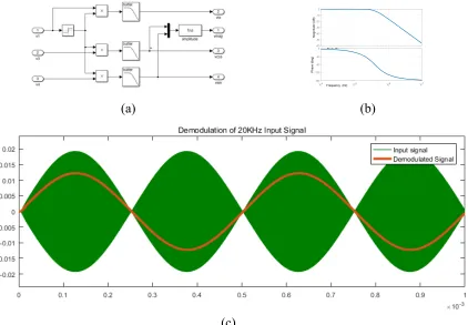
Figure 2-12 (a) Demodulation function block. (b) Bode plot of low pass filter. (c) Reference signal and demodulated signal. ... 30

Figure 2-13 IAPS open loop system model ... 30

(12)

xi

Figure 2-15 Air gap step response ... 32

Figure 2-16 (a) Signal strength feedback loop; (b) Air gap step response. ... 33

Figure 3-1 (a) Signals with DC offset; (b) Sensor output error caused by DC offset ... 36

Figure 3-2 (a) Signals with amplitude mismatch; (b) Sensor output error caused by amplitude mismatch. ... 37

Figure 3-3 (a) Signals with harmonics; (b) Sensor output error caused by harmonics. ... 38

Figure 3-4 (a) Signals with quadrature phase shift; (b) Sensor output error caused by quadrature phase shift ... 39

Figure 3-5 Error by signal DC offset in three-phase sensor ... 41

Figure 3-6 Error by signal amplitude mismatch in three-phase sensor ... 42

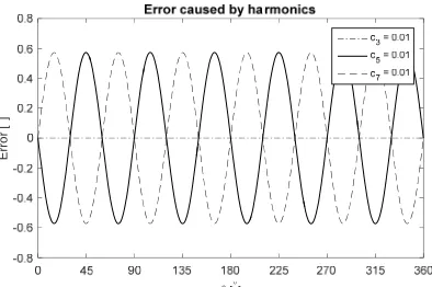
Figure 3-7 Error by signal harmonics in three-phase sensor ... 43

Figure 3-8 Error by signal phase shift in three-phase sensor ... 44

Figure 3-9 (a-d) the normalized high order harmonics of 2 pole to 5 pole, respectively. (e) linearity of two-phase and three-phase configuration. ... 45

Figure 3-10 Rotor profile with different 3rd harmonics ... 46

Figure 3-11 (a) 3rd_{and 5}th_{harmonics by different rotor shape harmonics. (b) corresponding} sensor output error. ... 47

Figure 3-12 (a) Input signal harmonics (b) Sensor error at different air gap ... 48

Figure 3-13 Rotor misaligned with IAPS coil ... 49

Figure 3-14 (a) & (b) normalized 3rd and 5th harmonics vs. rotor offset of two-phase configuration respectively. (c) & (d) sensor output error vs. rotor offset of three-phase configuration respectively. ... 50

(13)

xii

Figure 4-2 Box-Behnken design ... 54

Figure 4-3 Design parameters of (a) sensor coil, (b) rotor ... 57

Figure 4-4 Experiment configuration... 58

Figure 4-5 Response surface model of (a) Bias current, (b) TX voltage swing, (c) Linearity. ... 60

Figure 4-6 Pareto front of IAPS design ... 62

Figure 4-7 (A) ANSYS HFSS FEM model (b) ANSYS Designer SPICE model ... 63

Figure 5-1(a) solid rotor FEA model; (b) coil rotor FEA model. ... 66

Figure 5-2 Magnetic field strength when TX coil is driven by 50mW 4Mhz AC power. (a) solid rotor, (b) shorted rotor coil, (c) resonance rotor coil in-phase mode, (d) resonance rotor coil out-of-phase mode. ... 67

Figure 5-3 (a) simulation circuit; (b) tank current vs. rotor current. ... 68

Figure 5-4 Sensor configurations ... 69

Figure 5-5 Micro-inductive sensor equivalent circuit ... 70

Figure 5-6 Simulink model of MIAPS... 72

Figure 5-7 (a) eddy current; (b) receiving signal ... 73

Figure 5-8 operation region ... 76

Figure 5-9 Device cross section ... 76

Figure 5-10 micro coil fabrication process ... 79

Figure 5-11 probe station for device characterization ... 79

(14)

xiii

Figure 5-13 (a) Sensor assembly; (b) Rotor; (c) Test set up ... 81

Figure 5-14 (a) Sensor output transfer function; (b) Sensor linearity at different air gap. ... 81

Figure 5-15 (a) System in package design; (b) explosive view of substrate. ... 82

Figure 6-1 EPAS schematic arrangement. ... 83

Figure 6-2 (a) Steering torque sensor assembly. (a) sensor top view; (b) sensor iso view. .... 88

Figure 6-3 ISTS oscillator equivalent circuit ... 90

Figure 6-4 Mutual inductance (a) TX coil and rotor 1, (b) TX coil and rotor 2, (c) Rotor1 and Rotor 2 ... 91

Figure 6-5 Mutual inductance between the RX coils and rotors at different angle and air gap. ... 92

Figure 6-6 inductively coupled oscillator (a) Simulink model (b)SPICE model. ... 94

Figure 6-7 two oscillator (a) in opposite phase (b) same phase (c) quadrature phase (d) independently. ... 96

Figure 6-8 Steering torque sensor system model ... 96

Figure 6-9 (a) & (b) output for torsion angle of -8 and 8 degrees, respectively, (c) torsion angle output vs. steering angle, (d) torsion angle error. ... 100

Figure 6-10 (a) sensor output 1 when rotor 1 is fixed at different position and rotor 2 is rotating, (b) output 1 change caused by rotor 2, (c) cross-talk compensation, (d) residue cross-talk after compensation. ... 100

Figure 6-11 (a) & (b) Sensor 1 & 2 linearizer look-up table, (c) sensor output after linearization, (d) sensor linearity. ... 102

Figure 7-1 Inductive angle position sensor design. ... 105

(15)

xiv

Figure 7-3 (a) Equivalent inductance of coil L1 vs. rotor angle; (b) Fourier coefficient of inductance, C0 is not shown. ... 108

(16)

Chapter 1 Introduction

Automotive position sensor

A sensor is generally defined as an input device that provides a usable output in response to a specific physical measurand[1]. The measurand might be mechanical, electrical, magnetic, optical, chemical, acoustic, or a combination of any two or more of them [2], which affects the sensor in a certain way that causes a response represented by the sensor’s output. The output of many modern sensors is typically an electrical signal, but alternatively, could be a motion, deformation, or other usable type of output. Some examples of sensors include a thermocouple pair, which converts a temperature difference into an electrical output; a pressure sensor, which converts a fluid pressure into the deformation of a diaphragm [3]; a linear variable differential transformer (LVDT), which converts a position into an electrical output; and etc.

(17)

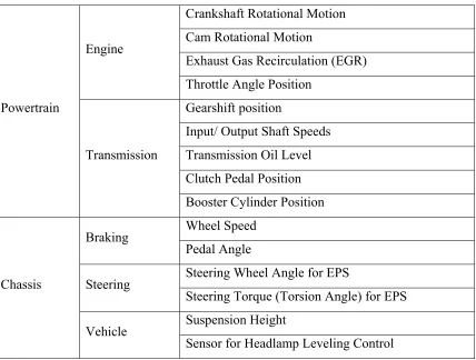
The application areas of automotive position sensors are mainly the powertrain, chassis and body systems [5]. Powertrain systems include the engine, transmission and all onboard diagnostics elements. Chassis systems include the suspension, braking, lightning, steering and stability systems. Body systems include the safety of occupants, comfort, information services, and in general the rest of systems aimed to fulfill the needs of the vehicle occupants [5, 6]. In the powertrain system, crankshaft and camshaft position sensors are used for the control of fuel injection and ignition timing, while the gear position sensor is applied in electronically controlled gear shifting to detect transmission gear position. In the antilock brake system (ABS) and the electronic stability program (ESP), wheel position sensor plays a major role in detecting wheel speed [7]. The position sensor is also a key element in “drive by wire” systems, active suspension, automatic headlight leveling, as well as in wiper, mirror and seat positioning. Another important application of position sensors is the detection of steering wheel position for autonomous driving systems. The main applications of automotive position sensors are summarized in table 1-1.

Table 1-1 Main Automotive Application of Position Sensors

Powertrain

Engine

Crankshaft Rotational Motion Cam Rotational Motion

Exhaust Gas Recirculation (EGR) Throttle Angle Position

Transmission

Gearshift position

Input/ Output Shaft Speeds Transmission Oil Level Clutch Pedal Position Booster Cylinder Position

Chassis

Braking Wheel Speed Pedal Angle

Steering Steering Wheel Angle for EPS

Steering Torque (Torsion Angle) for EPS Vehicle Suspension Height

(18)

Wiper Position Mirror Position

Body Safety Seat Position

Security Vehicle Tile for Anti-Theft System

With the advent of vehicle electrification, electric motors are gradually replacing the conventional mechanical and hydraulic systems [8]. The motor position sensor is another major application of position sensors. In brushless DC motors, field orientation control (FOC) regulates the commutation of the three phase current based on the rotor position. Minimizing the motor torque ripples depends on a smooth phase current commutation, which further depends on accurate rotor position information. The motor position sensor is essentially a high-speed angular sensor that can operate above 400 rpm with better than 0.5° accuracy and better than 0.1° resolution. Optical encoders or inductive resolvers are typically used for this application. The less expensive magnetic and inductive sensing technologies are gradually adopted while still generally meeting the technical requirements with lower performance margin [9].

1.1.1 Automotive position sensor requirements

(19)

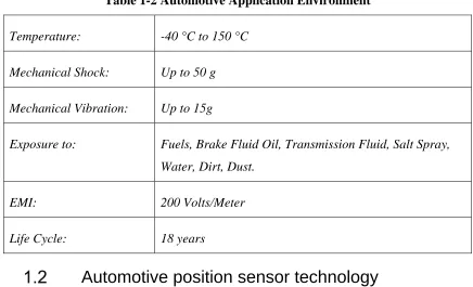
Table 1-2 Automotive Application Environment

Temperature: -40 °C to 150 °C

Mechanical Shock: Up to 50 g

Mechanical Vibration: Up to 15g

Exposure to: Fuels, Brake Fluid Oil, Transmission Fluid, Salt Spray,

Water, Dirt, Dust.

EMI: 200 Volts/Meter

Life Cycle: 18 years

Automotive position sensor technology

Based on the sensing technology, position sensors are classified in six major categories in the automotive applications sector, including resistive contacting sensor, Hall effect sensor, anisotropic magnetoresistive (AMR) Sensor, Optical Encoder, Integrated Magnetic Concentrator (IMC) Hall-Effect Sensor, and Inductive Position Sensor (IPS).

1.2.1 Resistive contacting sensor

(20)

1.2.2 Hall effect sensor

In an appropriate magnetic circuit, Hall sensor voltage varies with the angle between the flux density acting on the sensor and the bias current applied to the sensor. Typically, two Hall sensing elements are mounted in quadrature. The two Hall elements provide output signals, with one varying as a sine wave and the other as a cosine wave. The output signal is derived from the inverse tangent of the ratio of the quadrature element signals. This provides a linear indication of the angular position of the excitation field of the magnet,

thereby determining the angular position of the shaft [22]. Hall sensors are also used for linear position measurements, where magnet “head-on” and “slide-by” movements detect linear position [13].

1.2.3 Anisotropic Magnetoresistive (AMR) Sensor

The sensor exhibits changes of resistance as an external magnetic field rotates with respect to its sensing-elements. Two sets of four sensing elements are typically used. One set is physically offset from the other by a 45 degrees of angle. This angular offset again produces a quadrature 90 degree electrical phase angle difference. The two sets of sensing elements are connected in Wheatstone bridge signal-detection IC circuits. Both bridge circuits respond to the orientation of the external magnetic field and yield output signals. From these signals, the inverse tangent of their ratio gives a linear measurement of the angular position of the magnet target. The electrical angle goes through two cycles as the angular position of the magnet rotates one revolution. Further detailed information on AMR position sensors can be found in [23].

1.2.4 Optical

Encoder

(21)

wheel by starting with the position indicated by the potentiometer and then refining the calibration based on a period of straight-road driving.

1.2.5 Integrated Magnetic Concentrator (IMC) Hall-Effect Sensor

This sensor measures angular position using a single bar magnet attached to the rotating part whose angle is to be determined. The sensor is mounted on a fixed surface underneath the magnet. The sensor combines standard planar Hall effect technology with a unique Integrated Magnetic Concentrator(IMC) consists of the following components as shown in Figure1-1, this is done by with a detailed description provided for each.

Figure 1-1 IMC Hall-Effect Sensor

(22)

resolution of a combination of IMC-Hall element can be 10 times higher than that of the Hall element alone.

b) Hall-effect sensing elements: Hall-effect sensing elements are mounted on the silicon substrate, in four quadrant positions, below the IMC layer. Hall sensing elements detect the X and Y components of the magnetic field. As the magnet target rotates, pairs of Hall-effect sensing elements detect and generate quadrature and signal voltage waveforms [14].

c) Embedded digital signal processors (DSPs): The signals are in phase quadrature and are processed to determine a resolved angle with the inverse tangent function. DSPs are embedded on the silicon substrate along with the Hall effect sensing elements. Dual-DSP isolated dies are used for redundancy to ensure reliability [15].

The IMC rotary position sensor provides the following features: —Noncontact, easy-to-install, end-of-shaft mounting.

—Compact size, small outline package (excluding the magnet).

—Insensitivity to variations of magnetic field strength, temperature, and air gap. —Absolute 360 degree angular position measurement.

1.2.6 Inductive Position Sensor

(23)

Current flowing in the radial portions of the rotor conductor lobes generates a secondary magnetic field pattern that rotates with the rotor and inductively couples to the underlying receiving coils. Each of the receiving coils couples with the rotor magnetic field and inductively generates its own (phase-shifted) voltage waveform as a function of the rotor angle. The angle of the measured part (e.g., a throttle plate) is determined via signal processing of the magnitudes, signs, and gradients of the individually phase-shifted receiving-coil voltages [11], [12].

Inductive position sensors offer the following features: —Noncontact operation;

—No magnets are required;

—Low cost due to printed circuit board (PCB) structure; —Allow relaxed assembly alignment tolerances;

(24)

accelerator pedal sensors, steering angle position sensors, head lamp position sensors, etc. due to their mechanical variability (linear, rotational...), high temperature range, simplicity and robustness[11].

Objectives

Due to their outstanding merits, inductive sensors are most suitable for automotive applications where cost and flexibility are critical factors. They have been playing an important role in the automotive sensor family, and more and more automotive applications are switching to inductive sensing technology recently [12-14]. However, inductive position sensors are still not used as widely as magnetic position sensor in the automotive sector. One reason for the relative scarcity of inductive sensors is that their winding pattern makes them relatively big, especially for high accuracy devices that require precise winding. Another technical challenge is the designing of the optimal winding pattern and the rotor shape. Besides, the analysis of the inductive sensor performance heavily relay on Finite element analysis (FEA), which is very time-consuming.

To tackle these technical challenges, a design methodology for a robust and cost-effective inductive position sensor is developed in this work. A mathematic model for the sensor system is essential to understand the dominating factors of the sensor performance. Meanwhile the relation between the sensor raw signal quality and the sensor error need to be understood systematically to improve sensor accuracy. Since the design optimization of the inductive position sensor involves numerous design variables and optimization goals, an efficient optimization method specific for the inductive position sensor needs to be developed.

The objectives of the present work are multifold:

(1) the development of lumped mathematic model of inductive position sensor, which will be used as analytical tool for inductive sensor design and optimization;

(25)

(3) the developments of steering torque sensor and its experimental verification to demonstrate the inductive position sensor fusion;

(4) study of a passive inductive position sensor.

The underlying common theme of these objectives is the use of inductive sensing technology.

Thesis

Outline

The reminder of this work is organized as follows.

In section 2 we present the theoretical modeling of inductive position system including the electromagnetic structure, the oscillator circuit and the signal processing. The result is further verified by FEA and SPICE numerical simulation. A sensor system SIMULINK model is developed to present the transient behavior.

In section 3 we analyze the sensor error introduced by the imperfection of sensor raw signals for both two-phase and three-phase configurations. The corresponding correction method is also proposed.

In section 4 we optimize the sensor performance based on the response surface methodology. The method allows us to get an optimal design efficiently.

We develop a miniaturized inductive angular position sensor in section 5, which includes the modeling, numerical simulation, microfabrication process development and experiment validation.

We propose a steering torque sensor in section 6, the challenge and the potential the fusion of multiple inductive sensors are discussed.

(26)

Chapter 2 Theory and Modeling of Inductive Sensor

Background

An inductive angular position sensor (IAPS) typically comprises an electromagnetic structure and a support circuit[15, 16], which is commonly used to detect the angular position of the target relative to the reference. The electromagnetic structure consists of a transmitting coil, a certain number of receiving coils and a conductive rotor, which interact with each other through inductive coupling. The circuit provides power to sustain an alternating magnetic field, and it also conditions the receiving signal for Analog/Digital (A/D) conversion. The digitized signals are then used to calculate the angle, which is mapped into the desired output type. The output could be analog, Pulse Width Modulation (PWM) or digital format such as Inter-Integrated Circuit (I2_{C), Single Edge Nibble}

Transmission (SENT) or Serial Peripheral Interface (SPI).

To optimize the sensor performance for a specific application, it is critical to model the sensor system that includes both the electromagnetic structure and circuit. Numerical modeling is a popular method to model the IAPS system. The electromagnetic structure can be modeled by FEA, and the impedance matrix of the structure is derived after solving the electromagnetic field with a proper excitation at the coil terminal. The derived impedance matrix is then used in SPICE for circuit simulation. Such method provides good insight of the sensor performance from the perspective of both the electromagnetic field and the circuit. However, both FEA and SPICE circuity simulations are very time-consuming, and therefore, they are not practical when a large variation of design parameters needs to be investigated for sensor performance optimization.

(27)

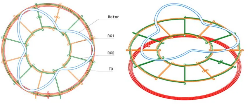
Sensor electromagnetic structure configuration

The minimal configuration of the electromagnetic structure of an IAPS, as shown in Figure 2-1, consists of a transmitting coil (TX), a conductive rotor indicating the target position, and at least two set of receiving coils (RXs). In the two-receiving-coil setup, the RXC coil receives a cosine signal of the rotor position and the RXS coil receives a sine signal of the rotor position. The rotor position can thus be calculated from the arctangent function of these two receiving signals. In some other configurations, three receiving coils are used to achieve better sensor performance. The benefit and signal processing of using three receiving coils will be discussed later in chapter 3.

Figure 2-1: IAPS electromagnetic structure top view and isotropic view

Sensor

Working

Principle

(28)

axially symmetric as shown in figure 2-2(b). Thus, the receiving coils can pick up signals that represent the coupler position.

(a) (b) (c)

Figure 2-2: (a) Excitation magnetic field; (b) Magnetic field modulated by eddy current; (c) Receiving coil winding.

Since the cross section of the excitation coil is much smaller than the coil’s length, the coil can be treated as filamentary wire. The magnitude of the resultant magnetic field generated at location

r



by current I passing through the excitation coil can be computed by using the

Bio-Savart law[17], as



_ 



TX

C p

x r

x r x Id r

B 0 ( ₃ )

4 )

( _ _ 

 

(2-1)

where path C_TX is the center line of the transmitting coil, dx is the differential element of the wire in the direction of the current. Since path C_TX is axially symmetric, the primary magnetic field induced by the transmitting coil B_p(r) is also axially symmetric, as demonstrated in Figure 2-2 (a).

When a conductive rotor loop is exposed to the excitation magnetic field, the induced voltage on the loop can be expressed by using Faraday's law of induction,



 

 

RT

dS B dt

d

(29)

where _RT is the area enclosed by the rotor profile. Consequently, an eddy current is induced on the rotor loop, i.e.,

R V

I  (2-3)

where R is the rotor loop resistance. The eddy current of the rotor can further generate a

secondary magnetic field, which could be expressed as,



_ 



RT

C S

x r

x r x Id r

B 0 ( ₃ )

4 )

( _ _ 

 

(2-4)

where CRTis the rotor profile path. Since the rotor profile is not axially symmetric, the

secondary magnetic field induced by the eddy current is not axial symmetric either. The total magnetic field is the superimposition of the primary and the secondary magnetic fields, i.e.,

) ( ) ( )

(r B r B r

Bt p S

 

 _ _ _(2-5)

Consequently, the receiving coil picks up a voltage of





 

RX

dS B dt

d

VRX t (2-6)

where RXis the area enclosed by the receiving coil.

Although FEA can be used to calculate the sensor signal and performance, it is generally very time-consuming. In the design stage, a wide design variation including different design parameters at different geometrical positions needs to be assessed. An accurate equivalent circuit will help us gain more insight on the critical factors of design and speed up the optimization procedure.

(30)

can be modeled as an inductor L₁and a resistor R₁ connected in series, and the rotor can

also be modeled as an inductor L₂ and a resistor R2 connected in series. The TX and the

rotor are inductively coupled through the mutual inductance M12.

Figure 2-3 Inductive torque sensor equivalent circuit

The TX is energized by an oscillator, which is modeled as a nonlinear resistor, as shown in Figure 2-3. When an alternating current passes through the TX, an eddy current is induced in the rotor through the inductive coupling. The mutual inductive coupling between the TX and the rotor can be modeled from the transformer equation and Kirchhoff's voltage law (KVL) as,

 

   

 

   

    

 



 



0

2 2 1 12 2

2

1 1 1 2 12 1

1

R t i t i dt

d M t i dt

d L

t v R t i t i dt

d M t i dt

d L

(2-7)

where i₁

 

t and i₂

 

t are the branch current through the TX and the rotor, respectively;v₁

 

t

is the voltage across the TX.

(31)

 

         t i dt d M t i dt d M t v t i dt d M t i dt d M t v 2 24 1 14 4 2 23 1 13 3 , ,     (2-8)

where M₁₃ and M₁₄are the mutual inductances between the receiving coils and the TX

coil, which are independent of the rotor angle since the TX is axially symmetric; M23

 



and M₂₄

 

 are the mutual inductances between the receiving coils and the rotor, and both

are depend on the rotor angle position.

When the TX coil is axial symmetrically wound, and the RX coil consists of clockwise and counter-clockwise segment interlaced alternatively, the mutual inductance between the TX and the RX disappears, i.e., M₁₃=M₁₄=0, due to the geometrical symmetricity. Equation

(2.8) is thus reduced to,

 

       t i dt d M t v t i dt d M t v 2 24 4 2 23 3 , ,     (2-9)

Therefore, the rotor angle position can be derived from signals v₃

 

,t and v₄

 

,t . In

practice, since the geometric relation between the RX coils and the rotor repeats after a maximum angle of 2π, the mutual inductance is a periodic function of the angle. It is convenient to design the geometry of the RX coils and the rotor so that their mutual inductance is a sinusoidal function of the angle, i.e.,

 

         p p N k M N k M cos sin 24 23 _(2-10)

where the pole numberN_pis defined as the number of the periodic features of the RX and the rotor. From equations (2-6) and (2-10), the rotor angle can be derived as,

   



v t v t



a

N_p tan2 , , ,

1

4

3  

(32)

Equation (2-10) shows that the two RX coils have identical geometry, with /2Npangle

offset from each other. The advantage of such a configuration is that the sensor accuracy only depends on the mutual inductance between the RX and the rotor, which will greatly reduce the design complexity.

Electrical

property

Equations (2-7) and (2-9) define the sensor signal. In order to solve the system of equations, the electrical properties used in the equations need to be solved first. This section provides an analytical solution for the electrical properties based on the geometry. Meanwhile, the excitation signal strength can be found by solving the governing equations of the oscillator circuit.

2.4.1 Mutual Inductance

The sensor output relies on the mutual inductances between the rotor and RX coils, which is further determined by the geometry of the rotor and the RX coils. It should be noted that the RXC is a quadrature electrical degree offset of the RXS; therefore, only one set of RX coil needs to be studied.

(a) (b) (c)

Figure 2-4 (a) Rotor at position (b) and (c) clockwise and counter-clockwise winding of RX coil respectively.

Figure 2-4 shows that the receiving coil can be further decomposed into a clockwise winding C₁and a counterclockwise windingC2. WindingC2offsets windingC1 by N_p

(33)

p

N pole design. Therefore the mutual inductance at position  between the rotor and the

RXC can be computed by using the Neumann formula:

 

 

 

)

( 1 2

2 1 0 2 1 4 ) (     rt

C C C r r

r d r d

M _ _

 

(2-12)

where C_rt()is the rotor profile path at position .

Because of the geometrical relation between C₁andC2as interpreted above, equation

(2-12) can be further simplified as:

             

 

)

( 1 2

2 1 0 1 4 ) ( ) ( ) ( ) (         rt p C C N r r r d r d M M M M     _(2-13)

Equation (2-13) shows that the sensor output can be fully determined by the double line integral between a receiving coil path C₁ and the path of rotorC rt ( ) .

Due to the geometrical periodicity and symmetry, the mutual inductance M ( ) is an even function with a period of

p

N



2 _{. It can be expressed in Fourier series as:}



    0 ) cos( ) ( i p i iN C

M



(2-14)

When the clockwise winding C1 and the counterclockwise windingC2 are combined

together, all even terms of the Fourier series are canceled out, and the mutual inductance between the rotor and the receiving coil is reduced to:



     0 1

2 cos((2 1) )

2 ) (

i

p

i i N

C

M



(2-15)

Equation (2-15) shows that the mutual inductance M() is not guaranteed to be a

(34)

will introduce error to the sensor output. The RX coil shown in Figure 2-4 is optimal since it uses the area most efficiently. The rotor geometry should match with the RX coil to get high signal strength and low high order harmonics. There is no analytical solution of the corresponding rotor geometry for a given RX geometry, which will be optimized using the trial-error method. In the following study three simplest rotor geometries, including eccentric circular, sinusoidal and star shape, are investigated. All those three geometries can be described by two parameters. In the case study, R₁and R2for both the RX and the

rotor are set to 7.5 mm and 15 mm, respectively, while the air gap between the RX and the rotor is set to 2 mm. Figure 2-5 shows that the star shape has the highest mutual inductance and the highest harmonics, while the eccentric circle shape has the lowest mutual inductance and harmonics. The sinusoidal rotor shape has a good balance on both the mutual inductance and the high order harmonics; therefore, this shape is chosen for the rotor design. The profile of the sinusoidal shape rotor can be described by:





) ( ) ( )cos( ),0 2

( ₂1 ₂ ₁

2 1 2

1     

 R R R R N_p

R (2-16)

where R₁and R2are the max and the min radius of the rotor profile, respectively.

(35)

(c)

Figure 2-5 (a) Rotor geometry. (b) Normalized harmonics. (c) Mutual inductance.

2.4.2 Self-inductance

The self-inductance of a filamentary current loop can be approximated by the mutual-inductance of two loops that are spatially separated by the geometrical mean distance (GMD) of its cross section [18].

 

 

 

C C d _x _x

x d x d L 2 1 2 1 0

4  

 





(2-17)

where d is the self GMD. The GMD between two areas S₁ and S2 is defined as:

1 2 2

1 1 2

) ln( 1

)

ln( x dsds

S S d S S

 

 (2-18)

The self GMD of a rectangle of width a and height b is [19]:

 

12 25 tan 3 2 tan 3 2 1 ln 6 1 ln 6 ln

ln 1 1

2 2 2 2 2 2 2 2 2

2_ _ _ _ _ _ _ _

   b a a b a b b a b a a b a b b a b a

d (2-19)

It can be evaluated by a simplified equation (2.20) within 0.2% accuracy for any a and b

[19].

) ( 2235 .

0 a b

(36)

2.4.3 Resistance

At high frequency, the skin effect concentrates the current at the surface of the metallic wire, which reduces its effective cross section and increases the AC resistance. Figure 2-6 demonstrates the current density distribution of an 18 mm diameter circular copper wire with rectangle cross section of 800 µm by 35 µm at 4 MHz frequency in Maxwell 2D. The skin effect makes the current density at the edge of the wire 4 times higher than at the center of the wire.

Figure 2-6 Current distribution by skin effect

The resistance caused by the skin depth can be approximated as [20]

w

t

e

t

R

skin DC t

0 0

1

0



_





_





 









(2-21)

where t₀ and w are the coil thickness and width, respectively, and  is the skin depth

expressed by

 

 

f

 (2-22)

with



and



being the material resistivity and permeability, respectively, and f being the operating frequency.

(37)

conductors is smaller than the conductor width. This phenomenon is called the proximity effect [21]. Figure 2-7 demonstrates the current distribution of 4 adjacent copper wires simulated by Maxwell 2D, where the current tends to distribute at the most outside.

Figure 2-7 Current distribution influenced by proximity effect.

The additional resistance caused by the proximity effect can be evaluated by [22]

                2 101 1 crit DC prox R R   (2-23) With sheet crit R W P 2 0 1 . 3 _  

 (2-24)

where critis the frequency at which the current crowding become significant and sheet

R is

the metal trace sheet resistance. Therefore, the total AC resistance of the coil by the skin effect and the proximity effect can be evaluated by







































 







 2 101 0 0 0

₁

1

crit w t DC AC t

e

t

R





 (2-25)

2.4.4 Stray Capacitance

(38)

which limits the operating frequency of the sensor. The stray capacitance of a single layer air-core coil is numerically modeled in [23]. For a multilayer coil with N_a layers and N_t

turns per layer, the stray capacitance can be approximated as [24],

 



 



_      _ _ _ _ 



 l i m b

N C l m C i m

C t

1

2

1 ₁ ₂ ₁ ₁

2 (2-26)

where C_bis the parasitic capacitance between two adjacent turns in the same layer, and C_m

is the parasitic capacitance between the two different layers. The parasitic capacitances of the tightly wounded coil can be determined as [24],









_                



4 4 0 0 0 0 0 0 0 0 5 . 0 cos 1 cos 1  























h r r D C d r r D C r r i r m r i r b (2-27)

where D_i,r₀,_r,hare the average diameter of coil, wire radius, thickness, and relative

permittivity of strand insulation and the separation distance between the two layers, respectively.

FEA or an impedance analyzer can be used to find the impedance characteristic and the resonance frequency of the structure, from which the parasitic capacitance can be derived. However, the simulation results indicate that when the resonance frequency is much higher than the sensor operating frequency, the coil behaves as a pure inductor. Therefore, the parasitic capacitance can be neglected without introducing much error.

2.4.5 Validation

(39)

be noted that our model takes less than 5% computing time of the FEM. Therefore, this model will be used in the later analysis of this research.

(a) (b) (c)

Figure 2-8 (a) FEA model. (b) Mutual inductance between rotor and RX1 coil. (c) Mutual inductance between rotor and TX coil.

Table 2-1 Coil self-inductance and resistance comparison between FEM and model.

FEA Model difference L1 [µH] 3.163 3.162 ‐0.06%

R1 [Ohm] 1.415 1.411 ‐0.27%

L2 [nH] 68.921 68.835 ‐0.12%

R2 [Ohm] 0.1698 0.170 0.09%

Sensor Oscillator Driving Circuit

The transmitting coil needs to be energized by a resonant oscillator circuit to compensate for the Ohmic loss. The resonant oscillator typically consists of a frequency selective network or a resonator and a nonlinear amplifier. In an IAPS, the resonator is an LC tank circuit, where the TX coil inherently acts as the inductor and capacitor [11, 25]. Due to their relatively good phase noise performance, ease of implementation in integrated system, and differential operation, cross-coupled inductance–capacitance (LC) oscillators play an important role in the high-frequency sensor applications [26-30].

One implementation of the cross-coupled LC oscillator is a single differential-pair oscillator[27] as shown in Figure 2-7(a). The main advantage of this configuration is that the DC level shift enables a large oscillation amplitude [31]; therefore, this implementation is adopted when the oscillation amplitude is critical for an enhanced signal strength. The

3 -20

-15

120 -10 -5 0

2.5 100

5 10 15

80 20

gap [mm] 2

theta [degree] 60 ₄₀

1.5 20 ₀ ₁

FEM Model

1 1.2 1.4 1.6 1.8 2 2.2 2.4 2.6 2.8 3

gap [mm]

90 95 100 105 110 115 120 125 130 135

(40)

other implementation is a complementary LC-tank oscillator, as shown in Figure 2-7(b), which employs both NMOS and PMOS switching transistors. The advantages of the complementary LC-tank oscillator includes [32] twice the tank voltage swing for the same current consumption, a larger loop gain due to the contribution of both NMOS and PMOS trans-conductance, and a controlled voltage swing that is always within the supply rail.

(a)

(b)

(c)

Figure 2-9 (a) Single differential LC oscillator; (b) Complementary LC oscillator; (c) Cross coupled oscillator equivalent circuit.

The free-running oscillator is an autonomous system, which can be modeled as a voltage controlled nonlinear resistor and an LC tank as in Figure 2-7(c). When the oscillator is working in the current-limit regime the voltage amplitude is proportional to the bias current multiplied by the tank parallel losses[33]. The governing equation of the oscillator circuit is given as[34]

   

 

   

 

                t v S G S t i t v dt d C t v R t i t i dt d L n tanh (2-28)

where C,L,R are the tank capacitance, inductance and series resistance, respectively. v

 

t

is the voltage drop cross the capacitor, i

 

t is the branch current of the inductor L, Sis the saturation current of the nonlinear resistor, and G_n is the gain of the nonlinear resistor,

0 M4 M3 C Itail Vdd L/2 L/2 R/2 R/2 0 M4 M3 M1 M2 R L C Itail Vdd R L C

(41)

which is determined by the transductance of the NMOS and PMOS devices. To understand the circuit oscillation startup condition, linear analysis is conducted. Under small signal condition, the nonlinear resistor can be linearized as,

 

|() 0

tanh  

     t v n n t v G t v S G

S (2-29)

Equation (2-28) is reduced to (2.30) in a matrix form as,

 

_                           t v t i C G C L L R t v dt d t i dt d n 1 1 (2-30)

To ensure the oscillation starts autonmously, the equation system (2-30) must be unstable. It can be shown that when the following condition is met,

L RC

Gn  (2-31)

the real part of the eigenvalue of the matrix

            C G C L L R n 1 1

is positive, and G_nis large enough

to compensate for the Ohmic loss of R. When R C

L _

, a periodic oscillation with the angular frequency given by equation (2-32) will start up.

LC

1

0 

 (2-32)

The corresponding SIMULINK model of equation (2-24) is demonstrated in Figure 2-9 (a). The circuit was simulated with the following parameters:L4.2H , C470pF,

  3.6

R , S1mA and Gn 0.00161. With these selected parameters, the LC tank

(42)

A SPICE simulation with the same parameters is run to validate the model, with the result in comparison with the analytical solution shown in Figure 2-9 (c). The operating voltage of the SPICE simulation is 6.24V. The start-up transient profile of the oscillation voltage also deviates slightly. The error source includes the deviation of the current-voltage relation of the nonlinear resistor and the neglected parasitic conductance and the capacitance of the transistor devices. Based on the comparison, the analytical model is sufficiently accurate to analyze the steady state system behavior.

(a) (b) (c)

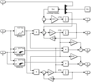
Figure 2-10 (a) Simulink model. (b) I-V curve of the oscillator. (c) Oscillator operating voltage.

IAPS Electromagnetic Structure Model

Based on the previous discussion, when a rotor is added into the system, the governing equations of the IAPS electromagnetic structure become

 

   

 

   

 

                       0 tanh 0 1 1 1 1 2 2 1 12 2 2 1 1 1 2 12 1 1 t v S G S t i t v dt d C R t i t i dt d M t i dt d L t v R t i t i dt d M t i dt d L n (2-33)

In the model, the excitation coil L₁ and the rotor L₂ are coupled through the mutual

(43)

 

                                                  t v t i t i G R R C L M M L t v dt d t i dt d t i dt d n 1 2 1 2 1 1 1 2 12 12 1 1 2 1 0 1 0 0 1 0 0 0 0 0 (2-34)

The analytic solution of the oscillation start up condition is quite difficult. However, for any given parameteres, we can check whether the real part of at least one of the eigenvalues

of the matrix

                        n G R R C L M M L 0 1 0 0 1 0 0 0 0 0 2 1 1 1 2 12 12 1

is positive. In the design stage, we

can use an approximated formula:

1 1 1 L C R k

Gn  (2-35)

where kis a safety factor greater than 1.

The receiving signal v₃ and v₄ are generated by the current on L₁ and L₂ through the

mutual inductanceM13, M23, M14 and M24. It can be expressed by,

 

         t i dt d z M t i dt d M t z v t i dt d z M t i dt d M t z v 2 24 1 14 4 2 23 1 13 3 , ) , , ( , ) , , (     13

M and M₁₄are all constants independent of the rotor position, while M23and M24 are

functions of air gap

z

and rotor angular position  .

(44)

Figure 2-11 IAPS electromagnetic structure model

Signal

Demodulation

The receiving signal is a high frequency signal, which needs to be demodulated and converted to digital format for further signal processing. One demodulation method is the synchronous peak detection, in which signals are sampled at the carrier’s peaks. In [35], a pair of quadrature carrier signals were used to demodulate the sensor signals. The signals were sampled using zero crossing detection of the 90 degrees phase shifted carrier signal. This method is attractive since it is simple and can demodulate the signal with no delay. However, the accuracy of this method is prone to the carrier noise.

The demodulation of this sensor uses the excitation signal v₁ as the synchronization

(45)

(a) (b)

(c)

Figure 2-12 (a) Demodulation function block. (b) Bode plot of low pass filter. (c) Reference signal and demodulated signal.

System

Model

Figure 2-13 IAPS open loop system model

The IAPS system model consists of a magnetic structure block (Figure 2-10), a signal demodulation block (Figure 2-11(a)) and a signal processing block. The signal-processing block calculates the angle from the sine and cosine signals. Figure 2-13 shows the

Phas

e (deg)

M

agnit

(46)

simulation result at a constant 2 mm air gap. The sensor can detect up to a maximum of 120 degree rotor angle since the output repeats every 120 degrees of the rotor angular position. In the first 30 µs sensor the signal strength gradually builds up. Sensor has low resolution during this transition stage, however sensor still has a correct output since the ratio of two signals remains correct.

(a)

(b)

(c)

Figure 2-14 (a) Receiving signal and demodulated signal. (b) Excitation current on transmitting coil and eddy current on rotor. (c) Rotor position and sensor output.

Signal

Strength

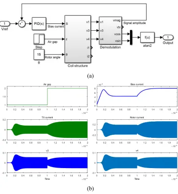
Feedback

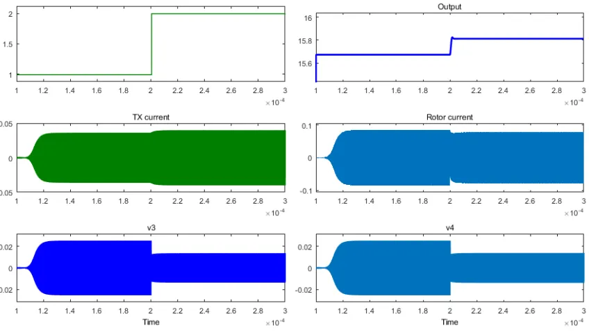
In operation condition the sensor might be subjected to geometric variation such as the air gap change. Such variation can cause the output signal change. Figure 2-14 shows the step response of the sensor air gap change. For a constant bias current S and a constant rotor

angle, when the air gap changes from 1mm to 2 mm, the excitation current increases due to the reduced load, and the eddy current on the rotor drops because of the reduced mutual inductance M₁₂. The receiving signals v₃and v₄drop by half because of the reduced eddy

current and reduced mutual inductances M23 and M24, however, the sensor output only

(47)

Figure 2-15 Air gap step response

(48)

(a)

(b)

Figure 2-16 (a) Signal strength feedback loop; (b) Air gap step response.

Conclusion

A mathematic model of the sensor system is developed in this chapter. The model is first simulated in SIMULINK, then validated by FEM and SPICE simulation. The results of the SIMULINK simulation agree very well with the FEM simulation. The model can be used for design optimization.

(49)

Chapter 3 IAPS

Error

Analysis

Accuracy is one of the key performance requirements for sensors. The output error of the IAPS is defined as the difference between the sensor position output and its real position. The allowable output error of the IAPS depends on its specific applications. Improving the accuracy of angular position sensors has received much attention in the literature [36-40]. In order to improve the accuracy of IAPS, it is essential to have a good understanding of its error sources. This chapter first investigates the output error caused by input signal error in two-phase and three-phase sensor configurations. The root causes of input signal error from the sensor implementation and sensor assembly are then studied. The final segment of this chapter discusses possible methods to improve IAPS accuracy.

Two–phase sensor output error

When the IAPS detects the angle from two input signals, this configuration is defined as a two-phase sensor [38]. In a practical sensor implementation, misalignment of the mechanical placement of the sensor board and the magnet can exist. In addition, there is part-to-part variation between the sensor devices if two discrete devices are used for generating signals with quadrature phase difference. Therefore, the resulting output signal from the sensor will contain undesired harmonics, amplitude variation and phase shift. The various irregularities cause the sensor output to deviate from the ideal case and thereby introduce various errors. In order to analyze the effect of these various signal irregularities on sensor accuracy, the errors are categorized as DC offset mismatch, amplitude mismatch, harmonics content of sine and cosine signals, and quadrature phase shift error. The sensor output error introduced by the signal errors is analyzed in the following part.

The output of the IAPS for an idea signal can be calculated by:

) , ( 2

tan x y

a



 (3-1)

(50)

 

    



sin cos 1 1 c y c x (3-2)

When the sensor signal deviates from the ideal signal, the sensor output becomes:

) , ( 2 tan ~ dy y dx x

a  





(3-3)

where dx and dy are the errors of the sine and cosine signals, respectively.

From Taylor’s expansion, the sensor output can be expressed as,

...

)

,

(

2 tan

)

,

(

2 tan

₂ ₂











y

x

ydx

xdy

y

x

a

dy

y

dx

x

a

(3-4)

Therefore the error of the sensor output can be determined as:

2 2

~

y

x

ydx

xdy















(3-5)

3.1.1 DC

Offset

The DC offset error in the sine and cosine signals is due to the unbalance between the clockwise and count-clockwise winding. The offset error causes the sine/cosine signal to have unbalanced positive and negative amplitudes and anomalies in the zero crossing. Assuming that the cosine and sine signals have c0_x and c0y DC biases, respectively, as

illustrated in Fig. 3-1(a), we have,

 

       y x c c y c c x 0 1 0 1 sin cos



(3-6)

From equation (3-5), the DC offset in the signals induces sensor output error as,

 



 



cos sin

1 0 1 0 c c c

c _y _x

 

(51)

(a) (b)

Figure 3-1 (a) Signals with DC offset; (b) Sensor output error caused by DC offset

Fig. 3-1(b) shows the errors caused by the sine and cosine signal DC offset, which have a phase difference of 90 degrees and thus cannot be canceled out. The period of the error caused by the DC offset is 360 degrees.

3.1.2 Amplitude

Mismatch

Ideally, both sine and cosine signals should have the same amplitude. Amplitude mismatch occurs when the geometry of the sine and cosine receiving coils are not identical. For instance, if the sine coil and the cosine coil are located at different PCB layers, the coil closer to the rotor will have greater amplitude. If the sine and cosine signals are defined as follows, where the cosine signal has higher amplitude than the sine signal by  percentage as illustrated in Fig. 3-3(a),

 



  

  

 









sin 1

cos

1 1 c y

c x

(3-8)

the corresponding sensor error can thus be derived from equation (3-5) as,

 









₂1

sin

2 

(3-9)

Error [

(52)

(a) (b)

Figure 3-2 (a) Signals with amplitude mismatch; (b) Sensor output error caused by amplitude mismatch.

Fig. 3-3(b) demonstrates the error caused by the amplitude mismatch; its period is 180 degrees.

3.1.3 Harmonic

Error

The sensor signals contain higher odd order harmonics. In particular, the geometrical mismatch and positional eccentricity between the coil and the rotor produce 3rd_{and 5}th

order harmonics. If the signals contain harmonics, as illustrated in Fig. 3-4(a), i.e.,

 











        

0 2 1

5 3 1 1 2 cos ... 5 cos 3 cos cos i i i c c c c x      (3-10)

 





 











            0 1 2 5 3 1 2 1 2 sin ) 1 ( ... 5 sin 3 sin sin i i i i c c c c x y        (3-11)

the corresponding error of the sensor is,

 

4 sin

 

8 ... sin 1 7 9 1 3

5



c c c c c

c  _ 



 (3-12)

Error [

(53)

In most cases, only the 3rd_{and the 5}th_{harmonics are significant, which dominate the} sensor accuracy.

(a) _(b)

Figure 3-3 (a) Signals with harmonics; (b) Sensor output error caused by harmonics.

Fig. 3-4(b) shows that the errors caused by both 3rd_{and 5}th_{harmonics have the same} period of 90 degrees, and therefore, the error will be canceled out when the harmonics have the same sign. This feature can be utilized to improve sensor accuracy.

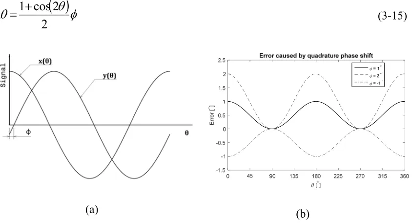
3.1.4 Quadrature Phase Shift Error

In ideal cases, the signals should exhibit a quadrature relationship. Due to the imperfect coil implementation, there could be a deviation from quadrature which causes additional error in the sensor output. The quadrature phase shift error  of two signals is defined below, and illustrated in Fig 3-5(a).

 





  

 







sin cos

1 1 c y

c x

(3-13)

The sine signal can be expressed in Taylor’s series:

 

cos

 

...

sin ₁

1  

c



c





y (3-14)

The error of the sensor caused by the quadrature phase shift error is thus determined as

Error [

Automotive Inductive Position Sensor

Scholarship@Western

Scholarship@Western