Accelerating MicroRNA Target Prediction Using Multithreading

Accelerating MicroRNA Target Prediction Using

Multithreading

Animesh Hazra1_{, Subrata Kumar Mandal}2_{, Soumyabrata Bhattacharyya}3_{, Aritra Dutta}4_{, Subham Jain}5 1

Assisstant. Professor, Computer Science & Engg. Department, Jalpaiguri Govt. Engg. College, Jalpaiguri, India. 2

Assisstant. Professor, Information Technology Department, Jalpaiguri Govt. Engg. College, Jalpaiguri, India. 3, 4, 5

Student, Computer Science & Engg. Department, Jalpaiguri Govt. Engg. College, Jalpaiguri, India

Abstract— MicroRNAs(miRNAs) are short, 21–23 nucleotide-long, single stranded RNA molecules that have been identified as one of the most significant molecules that regulate gene expression in various organisms which bind to 3' untranslated regions (3' UTRs) of their target mRNAs. The expression of miRNAs varies in different tissues, based on their functions. It is remarkably important to predict the targets of miRNAs by computational approaches to understand their effects on gene regulation and other biological functions. Various computational methods have been developed for miRNA target prediction. The available tools for miRNA target prediction encompass a range of different computational approaches, from the modelling of physical interactions to the inclusion of machine learning. It is crucial to adjust the Bioinformatics tools for more accurate target predictions, as it is equally important to validate the predicted target genes experimentally. CPUs having multiple cores are becoming increasingly popular and common nowadays. These are used for CPU intensive tasks and processing of complex data structures. We can employ it to speed up miRNA target prediction procedure. It can be a faster method. In this paper, we have explored the use of multicore CPUs to accelerate miRNA target prediction. We have executed our target prediction algorithm on multicore CPUs to parallelize it using multithreading.

Keywords — Bioinformatics, miRNA, Target Prediction, Gene Expression Regulation, Multithreading.

I. INTRODUCTION

Over the decades, the discovery of microRNAs (miRNAs) has totally changed our understanding of the complexity of gene regulatory networks. It is estimated that over half of mammalian protein coding-genes are regulated by miRNAs and most human mRNAs (Messenger RNA is a large family of RNA molecules that carry genetic information from DNA to other parts of the cell for processing i.e., ribosome sites for protein synthesis [3]) have binding sites for miRNAs [38]. Which genes are regulated by specific miRNA serves high potential biological knowledge. It serves a preliminary step in understanding the interaction of a miRNA with other genes and its functional position in regulatory mechanisms [4]. It is recognized from experimentally validated miRNAs and their target mRNAs that, they have high complementarity between them. Using this as a foundation, many algorithms have been developed to evaluate targets of specific miRNAs. Target prediction algorithms are mainly based on dynamic programming technique, machine learning, the free energy of the miRNA-target duplex and Hidden Markov Model (HMM).

Results obtained from these algorithms produce many false-positive target sequences [35][36][37]. True false-positives determine whether the two aligned sequences are genuinely homologous, whereas false positives determine whether they have been aligned by the algorithm by chance. If the alignment score falls below some threshold some of the alignments are not reported by the algorithm. We need to determine whether the sequences are true negatives (i.e., genuinely unrelated) or false negatives (i.e., homologous sequences that receive a score suggesting that they are not homologous). The goal of this paper is to develop an algorithm using dynamic programming that can estimate the miRNA targets with lower false-positive rates. Near perfect complementarity between miRNA and mRNA sequences eases the prediction of miRNA targets in plants. However, in animals it is really a challenging issue. Interaction between miRNA and mRNA lacks the perfect complementarity. This results in many different computational techniques to predict miRNA targets. A main goal of alignment algorithms is to maximize the sensitivity and specificity of sequence alignments. Sensitivity, also defined as the true positive rate (TPR), is the ratio of experimentally validated miRNA-target gene interactions predicted by an algorithm i.e., the number of true positives divided by the addition of true positive and false negative results. Also, Specificity is equal to 1 - false positive rate (FPR) which is defined as the ratio of false miRNA target gene interactions detected by an algorithm as being true i.e., the number of true negative results divided by the sum of false positive and true negative results [5]. Sensitivity is a measure of the ability of an algorithm to correctly identify genuinely related sequences whereas Specificity describes the sequence alignments that are not homologous. The performance of the algorithm is defined as the product of specificity and sensitivity. Most of the approaches used for miRNA target prediction are similar [36]. Some of the prediction criteria are:

1) The miRNA and 3' UTR of mRNA sequence have complementarity between them, especially between the seed region, position 2-8 of miRNA and mRNA. 2) The thermodynamics of miRNA and mRNA

interaction can be assessed by currently accessible RNA folding packages. Many prediction algorithms exploit this fact for target prediction [36].

We have accelerated the target prediction algorithm using multi-threading. The performance of multithreading depends on processor architecture, thread parallelism etc. If several threads work on the same dataset, they can actually share their cache. It ultimately leads to better cache usage or synchronization on its values. If an application does not exhibit sufficient amount of parallelism for multithreading, the processor utilization will not increase. Even if parallelism exists, the sharing of processor resources i.e., caches, functional units, etc., among threads, the context switching costs and the overhead of thread management and scheduling may hinder the overall performance [11][40].

A.Seed Match

MicroRNAs regulate the gene expression by binding to the mRNA. The seed sequence is essential for the binding of the miRNA to the mRNA. The seed sequence of a miRNA is defined as the first 2–8 nucleotides starting at the 5' end and counting toward the 3’ end. Even though base pairing of miRNA and its target mRNA does not match perfect, the seed sequence has to be perfectly complementary. When adenosine (A) pairs with uracil (U) and cytosine (C) pairs with guanine (G) then a perfect match occurs between a miRNA and mRNA sequences. A perfect seed match between the miRNA and the mRNA target has no gaps in alignment in the 2-8 region. Depending on the algorithm, various types of seed matches can be considered. The following types are the main types of seed matches [6][9]:

1) 6mer: A perfect match for six nucleotides between the miRNA seed and mRNA sequence.

2) 7mer-m8: An exact match to positions 2–8 of the mature miRNA seed.

3) 7mer-A1: A perfect match from nucleotides 2–7 of the mature miRNA seed followed by an A.

4) 8mer: A perfect match from nucleotides 2–8 of the mature miRNA seed followed by an A.

B.Different Regions of mRNA

Fig. 1. mRNA structure, approximately to scale for a human mRNA [3].

Figure 1 shows three main regions in a mRNA sequence, 3’ UTR, 5’ UTR and the CDS region. The coding region of a gene, alternatively known as the coding sequence or CDS (from coding DNA sequence), is that portion of a gene's DNA or RNA, that codes for protein. The untranslated areas of mRNA are non-protein-coding. It indicates that their sequence is not read as codons relating to a specific amino acid. The significance of these untranslated regions of mRNA is just beginning to be understood [3]. Recent researches have reported some connections between mutations in untranslated

regions and increased risk for growing a specific disease, such as cancer.

C.Local Alignment Algorithm

The local alignment algorithm uses the Dynamic Programming technique. The local alignment algorithm of Smith and Waterman (1981) is the most exhaustive method by which subsets of two protein or nucleotide sequences can be aligned. Local alignment is extremely useful in a variety of applications like database searching. A local sequence alignment algorithm resembles global alignment in sense that two proteins are arranged in a matrix and an optimal path along a diagonal is sought. However, there is no penalty for starting the alignment at some internal position, and the alignment does not necessarily extend to the ends of the two sequences [7].

In Smith–Waterman algorithm similarity matrix is constructed with an extra row along the top and an extra column on the left side. For sequences of lengths m and n, the matrix have dimensions m + 1 and n + 1. The score in each cell is selected as the maximum of the preceding diagonal or the score obtained from the introduction of a gap. However, the score cannot be negative. If all other score options produce a negative value, then a zero must be inserted in the cell [7]. We consider the gap penalty as a negative value. The score M[i,j] is given as the maximum of four possible values:

1) The score from the cell at position i – 1, j – 1, that is, the score diagonally up to the left. To this score, add the new score at position s[i,j], which consists of either a match or a mismatch.

2) M[i, j – 1] (i.e., the score one cell to the left) plus a gap penalty.

3) M[i –1, j] (i.e., the score immediately above the new cell) plus a gap penalty.

4) The number zero.

This condition ensures that there are no negative values in the matrix. In contrast, negative numbers commonly occur in global alignments because of gap or mismatch penalties.

Fig. 2. Recurrence relation for Smith-Waterman (SW) algorithm.

From the above recurrence relation, the matrix is filled from top left to bottom right with entry [i,j] requiring the entries [i,j-1], [i-1,j-1], and [i-1,j]. By choosing the maximum value we make sure the best score is found and stored, so that the next entries are build up based on that.In this relation s[i][j] is the match/mismatch value.

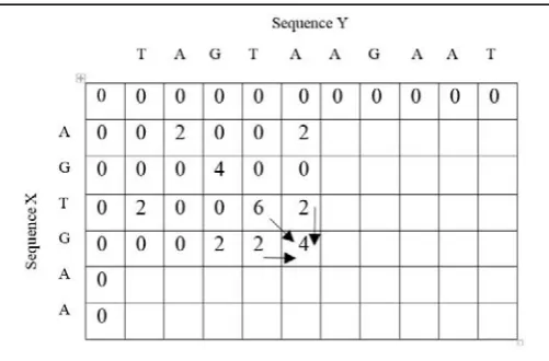
An example of the operation of local alignment algorithm to align two nucleic acid sequences are shown in Figure 3 and Figure 4 [10]. We have taken two sequences as Sequence X and Sequence Y respectively. The sequences are given below:

M[i][0] = 0 , M[0][j] = 0 ; 0.

 Sequence X – “AGTGAA”

 Sequence Y – “TAGTAAGAAT”

Also, Figure 3 shows the steps involved in computing the similarity matrix. Here, we assumed that the match score is 2, mismatch score is -2, and the gap penalty is -4. Figure 4 shows the local alignments with the optimal score (Scoreopt)

calculated using the equation number (1). The topmost row and the leftmost column of the matrix are filled with zeros.

Fig. 3. Steps involved in the calculation of similarity matrix using the

sequences X and Y.

The maximal alignment can begin and end anywhere in the matrix. The procedure is to identify the highest value in the matrix using the equation number (1). However, there can be more than one optimal score. More than one optimal score signifies that the sequences have more than one alignments. The trace‐back procedure begins with this highest‐value position and proceeds diagonally up to the left until a cell is reached with a value of zero. This defines the start of the alignment, and it is not necessarily at the extreme top left of the matrix.

Scoreopt =max (M[i][j]) (1)

i.e.,

Fig. 4. Local alignment of the sequences X and Y with the optimal score

using Smith-Waterman (SW) algorithm.

Here, 6 is the maximum score so we start all the alignments from the cell having the value 6. We then backtrack the matrix until a zero is found.

Fig. 5. Possible aligned sequences obtained from the given nucleotide

sequences.

The aligned sequences obtained by aligning Sequence X and Sequence Y are shown in Figure 5. During backtracking we move in opposite direction. If the score is obtained from its immediate diagonal or upper or left cell, we proceed along that path.

D. miRNA– mRNA Interactions

sequence. There is no single model that would depict all miRNA-mRNA interactions as they are relatively heterogeneous. At least 6-7 nucleotides consecutively paired in positions 2-8 of miRNA are usually required to improve the effectiveness of miRNA-mRNA interaction which in turn facilitates target prediction. Securing more and more information about miRNAs and their role in gene regulation encouraged researchers to improve the way of analysing individual miRNA-mRNA interactions.

Fig. 6. miRNA and mRNA target interaction [6].

Figure 6 shows schematic overview of a miRNA interaction with its mRNA target [6]. The position number of the miRNA is shown in blue. The seed sequence refers to nucleotides in miRNA position number 2–8. Flank denotes the mRNA sequence on either side of the seed region. WC matches in the seed sequence are shown in red, and G-U wobble in the seed sequence is shown in green. In a wobble base pairing between two nucleotides in RNA molecules does not follow Watson-Crick (Guanine-Cytosine and Adenine-Thymine) base pairrules.

II. LITERATURE SURVEY

Early researches in the area of miRNA informatics focused on identifying miRNA genes along long strands. The problem is identified as investigating a region which represents a putative miRNA from given sequence [4]. A more challenging problem in the field is the validation of target genes for specific miRNAs. The difficulties in experimental validation of miRNA target genes have prompted the researchers to devise new computational methods to produce potential targets. The problem has been widely studied over the decade [39]. Most of the available methods use sequence information coming from miRNA and potential mRNA targets. Due to presence of perfect complementarity between miRNA sequences and mRNA targets, the problem is easily tractable in plants. However, in animals most miRNAs are not perfectly complementary to their targets, so the process cannot be easily explained. Some recent researches attempted to use gene expression data to evaluate the miRNA-target relationships. Current researches have already recognized that miRNAs have a certain effect on the expression level of the mRNAs that are established as their targets. Therefore, we can conclude that miRNA and mRNA should exhibit strong correlation if there is a binding relationship between them. Specific gene that are regulated by an individual miRNA provides high potential biological knowledge. It serves as a preliminary step in understanding the interactions of a miRNA

with other genes and it’s functional position in regulatory mechanism [4].

A. MicroRNA Target Prediction Tools

miRanda [12][13] looks for high complementarity between miRNA and mRNA for identifying potential binding sites. The scoring method used by the algorithm favors complementarity between 3' end of mRNA and 5' end of the miRNA. Using basic parameter settings the false-positive rate is between 24% and 39%.

miRanda-mirSVR [6][12] is an online tool that is a combination of two approaches. miRanda is used to recognize potential target sites and mirSVR is used to score them using an approach similar to SVM. It does not allow one to supply new data i.e. all the results are precomputed.

Support vector machine [21] uses machine learning approach for evaluating interactions between miRNA and mRNA. SVM is based on different features which can be classified into three elements: structural, thermodynamic and position based features. This method builds a statistical model and tries to validate miRNA targets by fitting miRNA and their targets in the model.

TargetScan and TargetScanS [14][15] method checks for complementarity in the seed region. Also, it checks the complementarity in other regions. In the beginning of the prediction process it tries to filter many false-positives. Also, it uses conservation criteria for filtering. Predicted binding sites are then validated thermodynamically. TargetScanS is the improved version of TargetScan. The estimated false-positive rate is between 22% and 31%.

MirTarget2 [34] uses features extracted from a large microarray training dataset for predicting different miRNA targets. It makes target prediction using SVM [6].This machine-learning approach uses several popular prediction features like seed match, conservation, free energy, site accessibility etc. MirTarget2 predictions can be obtained from miRDB.

PicTar [16][17] algorithm uses a group of orthologous 3' UTRs from multiple species and then scans it for those displaying seed match to miRNAs. Then the matched alignments are filtered according to their thermodynamic stability. Predicted targets are then scored using Hidden Markov Model (HMM) maximum-likelihood fit approach. DIANA-microT[18][19][20] was one of the first miRNA target prediction tool to predict targets in humans. This method uses a 38 nucleotide window that gradually moves across a 3' UTR sequence. It also calculates free energy of binding sites for target prediction [29]. Instead of 5' end complementarity it takes into account the 3' end complementarity to the miRNA.

independent test dataset the sensitivity and specificity becomes 76.5% and 66.1%.

Probability of Interaction by Target Accessibility (PITA)[23] focuses on the features like seed match, free energy, site accessibility, conservation, and target-site abundance for target prediction. However, it uses target-site accessibility as the major feature for miRNA target prediction. At the preliminary step PITA recognizes a potential site by seed match criteria. It then considers site accessibility by computing a free energy score of the miRNA and its targets. Thereafter, target site abundance is considered [6].

RNAhybrid [25][26] is based on features like seed match, free energy and target-site abundance etc. It takes a user defined seed region and considers the free energy between a miRNA and its targets. Various advanced features are provided by the tool like specification of hits per target, helix constraints, maximal bulge loop size, maximal internal loop size and maximum free energy cutoff [6].

Although these tools use a combination of features to compensate for the shortcomings, each of these tools has its own merits and demerits. In terms of their wide range of capabilities, ease of use, comparatively current input data and maintenance of the software, three of these tools surpasses the others. These are miRanda-mirSVR, DIANA-microT-CDS and TargetScan. All of these tools are updated periodically over the last several years and are easy to use [6].

B.MicroRNA Target Gene Databases

MicroRNA database and microRNA targets databases is a collection of databases and web portals and servers used for microRNAs and their targets.

StarBase [28] focuses on miRNA-lncRNA, miRNA-mRNA, miRNA-circRNA, miRNA-pseudogene, miRNA-sncRNA, protein-lncRNA and protein-sncRNA interactions.

TargetScan [14] predicts biological targets of miRNAs by searching for perfect match in the seed region of each miRNA. In flies and nematodes, based on the probability of their evolutionary conservation the predictions are ranked. In mammals and nematodes, the user can chose to extend the predictions beyond conserved sites and consider all sites. TarBase [30] database contains experimentally tested and

validated miRNA targets, in humans/mice, fruit fly, worms, and zebrafish.

miRTarBase [31] is experimentally validated microRNA-target interactions database with up-to-date results. It contains experimentally validated data on various species.

C.MicroRNA Databases

miRBase [32] database is a searchable database of published miRNA sequences and annotation. microRNA.org [12] is a database for experimentally validated microRNA expression patterns, predicted microRNA targets and target downregulation scores.

miRDB [33][34] is an online database which mainly focuses on functional annotation as well as miRNA target prediction. Functional annotations are reported with a primary focus on mature miRNAs.

However many more database like miRNAmap, PhenomiR, miRecords, miRWalk etc are also available.

III. PROPOSED ALGORITHM

Input:

1. Number of threads. 2. MicroRNA sequence. 3. DNA Sequence in 3’ UTR.

Output:

Aligned sequences greater than a certain threshold value.

Step 1: Compute the complement of the DNA sequence

i.e., the A (Adenine) is complemented to U (Uracil) and C (Cytosine) to G (Guanine) and vice versa to get the mRNA sequence. Also reverse the sequence for target prediction.

Step 2: Compute the number of sliding windows and

assign equal number of sliding windows to each thread. It can be done in the following ways:

a) Compute the total number of sliding windows. b) Divide the total number of sliding windows (say

w) by the number of threads (say t) and assign it to X.

c) Assign X number of sliding windows to each thread.

d) If w modulus t is not equal to 0, i.e., w/t has a remainder, then assign these remaining windows to the final thread.

Step 3: Generate sequences equal to the size of the

miRNA sequence by sliding window approach in each thread.

Step 4: Assign the match value, mismatch value, gap

penalty in the 2-8 region (seed region) of the miRNA greater in magnitude than the values in rest of the regions. Compute local alignment with the sequences.

Step 5: Write all the alignments greater than the threshold

value.

Step 6: Observe the 2-8 region of the miRNA sequence in

the alignments.

a) If there is a contiguous pairing in the seed region we conclude that it is a true positive pair.

b) If there is no contiguous pairing in any of the alignments, we conclude that it is a false positive pair.

IV. EXPERIMENTAL RESULTS

For performance analysis, the algorithm was tested in different types of processors to observe how the algorithm utilizes the multi-threading concept, carried by the different multicore CPUs. Table. I displays the different processors, on which the algorithm was tested. We have taken the following gene sequence and a miRNA sequence.

We get the target mRNA sequence from the input gene sequence. Finally, we compute the local alignment between the mRNA and microRNA sequences.

The input gene (DNA) sequence is as follows:

>NM_173647 Gene NAME: RNF149 GeneID: 284996

“ACACGTGCCCACTGAAGTGGCACCAACAGAAGTTT GGCTTGAACTAAAGGACATTTTATTTTTTTTACTTTA GCACATAATTTGTATATTTGAAAATAATGTATATTAT TTTACCTATTAGATTCTGATTTGATATACAAAGGACT AAGATATTTTCTTCTTGAAGAGACTTTTCGATTAGTC CTCATATATTTATCTACTAAAATAGAGTGTTTACCAT GAACAGTGTGTTGCTTCAGACTATTACAAAGACAAC TGGGGCAGGTACTCTAATATAAAGGACAGGTGGTGT TTCTAAATAATTGGCTGCTATGGTTCTGTAAAAACCA GTTAATTCTATTTTTCAAGGTTTTTGGCAAAGCACAT CAATGTTAGACTAGTTGAAGTGGAATTGTATAATTCA ATTCGATAATTGATCTCATGGGCTTTCCCTGGAGGAA AGGTTTTTTTTGTTGTTTTTTTTTTAAGAACTTGAAAC TTGTAAACTGAGATGTCTGTAGCTTTTTTGCCCATCT GTAGTGTATGTGAAGATTTCAAAACCTGAGAGCACT TTTTCTTTGTTTAGAATTATGAGAAAGGCACTAGATG ACTTTAGGATTTGCATTTTTCCCTTTATTGCCTCATTT CTTGTGACGCCTTGTTGGGGAGGGAAATCTGTTTATT TTTTCCTACAAATAAAAAGCTAAGATTCTATATCGCA CATGAGCATTAAGTTCTTCATTGCCTTGTTAAGGAAA ATGAGTAGGCAGACTCAGAATCTGTTATATTGATTTC AGTTACAATTTAATCTTTACAATTAAAAGGGCGAAA GATGTAGAATTTTAGTTTTTGTTGTTGACTCGAAATA ACCAGTTTTCTTGATTAGAGTTTAAGCAGATTTAATA CCATGACCTTGCTTAACCGTTTCTTCTTTTTTACTTGC TTGCTGTTCTTTTGGGTCAAAGGAGCAGGCTAATGCA AAGCTTTTGGAGACTGCTAAGTGTTAAAAAGTGATT AAACACACACTCTGCTATTTTTTCACTTCTTGGAGGT AGAAGTCGAGTATGAGGCAGTTATTTTTTAGAGTGT GGAATTATAGTCTTTCCTTGCTCCTAGTTATTCTGTAT ATCTTTACTTTGTAGGTAAAAATAAATGTTTATTTAA AACAATTTTTAAAATTATAAATTTATTTTTATAGCCA TATGTAGGATATAAAGATTTATATAGATTATTTTCTC AAGCTACTTAATGCTTTAATTCTAGCTACTCATCATG AAATAGTAAACAGTTTTACTGAAATAAACTCTACAG ACAGATGCAGTATGAGGAGCTATTGAAGTAGAAAAT GTATTTCGCTTTGCACACTGAGTTGGTTTTAGCAGAC AACCTCAAGTAGGTTTCCATAACAGCCATTACCTTTG AAATCTACCTTCTGTAGTTTATTATAAATAGGAAAAT ACATCCTGATTCTGTAGCAAGTAGATTGTTTGCTCTT TGTCTTTAAGAAATACTAGGAGGGCCGGGCGCGGTG

GCTCACGCCTGTAATCCCAGCACTTTGGGAGGCCGA GGCGGGCGGATCACGAGGTCAGGAGATCGAGACCAT CCCGGCTAAAACGGTGAAACCCCGTCTCTACTAAAA ATACAAAAAATTAGCCGG”

The input mature microRNA sequence is as follows:

>hsa-miR-373 MIMAT0000726 Homo sapiens miR-373 “GAAGUGCUUCGAUUUUGGGGUGU”.

Here, we have used the scoring scheme such that in the 2-8 region of miRNA the match, mismatch and gap values are more than the rest of the regions. We used a match value of 14, mismatch value of -10 and gap penalty of -6 for the seed region. For other regions, these values are set to half of their values i.e. 7,-5 and -3 respectively. Here, the length of the mRNA sequence is 1636 and the length of miRNA sequence is 23. Let the number of threads be 3, so the mRNA sequence is divided into 3 parts. The total number of sliding window is m-n+1, where m is the length of the mRNA sequence and n is the length of the miRNA sequence. So, the value of m-n+1 will be equal to (1636-23+1) which is 1614. Now, we divide the total number of sliding windows by the number of threads which is denoted as X, where X indicates the number of sliding windows allocated to each thread. Therefore, the value of X is equal to (1614 / 3) i.e. 538. The mRNA sequence is divided into 3 parts from positions 0-559, 538-1097 and 1076 -1635. Here, the lower limit of the sequence is (X * i) and the upper limit of the sequence is (X * (i+1) + |miRNA| - 2) where ‘i’ denotes the number of iterations and |miRNA| denotes the length of the miRNA sequence. Also, ‘i’ varies from 0 to number. of threads minus 1. If the number of sliding windows is not a perfect divisor of the number of threads, then we compute the remainder which is equal to the number of sliding windows modulus number of threads. We add this remainder to the upper limit in the last sequence.

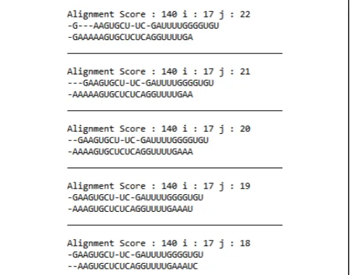
Fig. 7. Alignments obtained by the algorithm over the target sequence.

the miRNA sequence miR-373, we get alignments which is shown in Fig. 7 with a threshold value of 135.We observed the aligned sequences in Fig. 7 for contiguous pairing in the 2-8 region of the miRNA. There are no gaps in the seed region and hence it is contiguous. So, it is a true positive pair. Here, Alignment Score denotes the alignment score obtained during aligning the sequence. Also, ‘i’ and ‘j’ denotes the row and column of the cell in the alignment matrix where the highest score is found.

V. DISCUSSIONS

As more information about miRNA–mRNA interactions are becoming available, target prediction algorithms and publically available databases are continuously being developed. New publically available database tools are being developed to incorporate the new data [24]. A number of computational tools have been developed for miRNA target prediction over the decade. Here, we applied multithreading approach to analyse the seed region of miRNA for perfect matches with the target gene sequence. We know, local alignment using Smith-Waterman algorithm runs in O(n2₎

time. Despite of its high time complexity, it produces more accurate result than any other algorithms. So, we have used multi-threading technique to compensate for this high time complexity. We have provided a theoretical proof for the calculation of time complexity of our algorithm which is based on three assumptions. The assumptions are given at the end of this section. We have shown the computation of single or multiple threads on different multi-core CPUs. We have cited the relationships between the number of threads and number of processors and the computation of perfect linear speed-up with different number of processors. Suppose, length of the mRNA sequence is m and the length of the miRNA sequence is n. Let, the size of each sliding window be n. Then, the total no of sliding windows will be m–n+1. Assume, each operation of Smith-Waterman algorithm takes k unit of time. Then, if it is executed serially (i.e., using single processor), it will take ((m–n+1)*k) units of time.

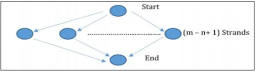
Computational diagram 1 is shown as follows:

Fig. 8. Computational diagram 1 (algorithm using single thread).

Figure 8 shows the execution of algorithm using single thread. If a sequence of instructions contain no parallel control then we may group them into a single strand, each of which denotes collection of one or more instructions. The instructions before the execution of Smith-Waterman algorithm are grouped into a single strand denoted by Start. After execution of Smith-Waterman algorithm, remaining instructions for computing results are grouped together to

form a single strand denoted by End. The (m-n+1) denotes the number of sliding windows the algorithm operates on. Thus, when all the tasks of a single thread are taken into account, we get a total of ((m-n+1) + 2) operations. Let us assume that it takes k units of time to execute Smith-Waterman algorithm once. Then the total time taken by the algorithm will be (k*(m-n+1)) plus time taken to execute Start and End strands. But, we know that each of the (m - n + 1) Smith-Waterman operation can be executed in parallel without any interference. This is shown in Figure 9. Thus, if there are (m - n + 1) processors, the entire operation will take k units of time plus the time taken to execute Start and End Strands.

Fig. 9. Computational diagram 2 (algorithm using multiple threads)

Let, Tp be the time taken by p processors to execute the

algorithm.

Let’s assume that the Start Phase and End Phase takes constant time, i.e. O(1).

Therefore,

T1 = Time taken by a single processor

= (m – n + 1) * k + 2 * O(1) ≈ (m - n + 1) * k

T∞= Time taken by infinite processors = k + 2 * O(1)

≈ k

However, if there are infinite processors we won’t achieve perfect linear speed up. We can achieve perfect linear speed up when exactly (m - n +1) processors are used.

Also as we know that [42],

Tp ≤ (T1/p) + T∞ (2)

From equation number (2) we get an upper bound on Tp.

Also, T∞(w) denotes the running time of executing ‘w’ sliding windows using infinite processors. Here, ‘w’ denotes the number of sliding windows. So,

T∞(w) = max (T∞(1), T∞(1)……… T∞(1)) = T∞(1)

= k (3)

Now, we know that each Smith-Waterman algorithm takes O(n2_{) amount of time. Thus, T}

∞(w) = k = O(n2) = c*n2 where c is a constant. Also

Here, T1(w) denotes the time taken by single processor to

execute ‘w’ sliding windows.

Therefore, Parallelism = T1 (w)/ T∞(w) (5)

Using equation number (3) and (4) in equation number (5) we get,

Parallelism = Θ(m-n+1).

Few optimistic assumptions that are necessary here are as follows:

a) At the time of execution of the program, all the processors are experiencing minimum possible load. b) The operating system equally distributes the load

among the processors.

c) Depending on the processor’s availability each thread will be executed by distinct processor.

We have executed the algorithm on different processors and it is shown in TABLE I.

TABLE I

EXECUTION OF THE ALGORITHM ON DIFFERENT ENVIRONMENTS

Processor , RAM Used No. of

Cores No. of Threads Intel® Core™ i3-3110M @2.40

GHz, 4GB RAM 2 4

Intel® Core™ i5-4210U @1.7 GHz,

2.4 GHz, 4GB RAM 4 4

Intel® Core™ i7-3610 QM @2.3

GHz, 8GB RAM 4 8

VI. CONCLUSION

A number of computational tools have been designed for miRNA target prediction but to choose a perfect tool is a challenging task in Computational Biology. There is no particular algorithm that can be used generally for every analysis of 3’ UTR sequences. Securing more and more knowledge about miRNAs and their role in gene regulation prompted researchers to devise ways of analyzing individual miRNA-mRNA target interactions. This paper focuses on developing a new computational method using dynamic programming and multi-threading to predict miRNA targets with more accuracy. The paper discusses the currently available computational methods in brief and proposes a new algorithm using the currently available knowledge about miRNA and mRNA interactions. We have explored the use of multi-core CPUs on target prediction. We tested this algorithm on CPUs having multiple cores and observed the results. The quality of target prediction with this method can be further improved by adding the more target predicting criteria’s like conservation, free energy etc. in future.

ACKNOWLEDGEMENT

We take this opportunity to thank Mr. Suman Ghosal and Mrs. Shaoli Das of Indian Association for the Cultivation of Science, Kolkata for their exceptional guidance and support. We would also like to thank Dr. Dipak Kumar Koley and Mr. Subhas Barman faculty members in the Department of Computer Science and Engineering. Jalpaiguri Govt. Engineering College, Jalpaiguri, for their valuable time and feedback during the preparation of this research paper.

REFERENCES

[1] Semih Ekimler and Kaniye Sahin, “Computational Methods for MicroRNA Target Prediction “; Genes 2014, Vol: 5, Pages: 671-683;

doi:10.3390/genes5030671.

[2] Suman Ghosal, Shekhar Saha, Shaoli Das, Rituparno Sen, Swagata Goswami, Siddhartha S. Jana & Jayprokas Chakrabarti, “miRepress: modelling gene expression regulation by microRNA with non-conventional binding sites”, Scientific Reports, 2016 Feb 29; 6:22334. doi: 10.1038/srep22334.

[3] https://en.wikipedia.org/

[4] Hasan Oğul, Mahinur S. Akkaya; “Data integration in functional analysis of microRNAs”, Current Bioinformatics, Dec 2011, Vol: 6,

Issue 4, Pages: 462-472, doi: 10.2174/157489311798072945.

[5] Yanju Zhang and Fons J. Verbeek; “Comparison and Integration of Target Prediction Algorithms for microRNA Studies”, Journal of Integrative Bioinformatics. 2010 Mar 25, Vol : 7 , Issue 3, Pages doi:

10.2390/biecoll-jib-2010-127.

[6] Sarah M. Peterson Jeffrey A. Thompson, Melanie L. Ufkin, Pradeep Sathyanarayana, Lucy Liaw and Clare Bates Congdon, “Common features of microRNA target prediction tools”; Frontiers in Genetics, 18 February 2014, Pages: 671-683 doi: 10.3389/fgene.2014.00023. [7] Jonathan Pevsner; “Bioinformatics and Functional Genomics” , Third

Edition, John Wiley & sons Inc., ISBN: 978-1-118-58178-0

[8] Bandyopadhyay, S., and Mitra, R. (2009). “TargetMiner: microRNA target prediction with systematic identification of tissue-specific negative examples”. Bioinformatics 25, Pages: 2625–2631. doi: 10.1093/bioinformatics/btp503.

[9] Wenlong Xu, Anthony San Lucas, Zixing Wang, Yin Liu; “Identifying microRNA targets in different gene regions”; BMC Bioinformatics

2014, Vol: 15 , Suppl 7: S4.

[10] Wellington S. Martins, Juan del Cuvillo Wenwu Cui and Guang R. Gao, “Whole Genome Alignment using a Multithreaded Parallel Implementation”, Proceedings of the Symposium on Computer

Architecture and High Performance Computing (SBAC), 2001, Pages:

1-8.

[11] Pramitha Perera and Roshan Ragel; “Accelerating Motif Finding in DNA Sequences with Multicore CPUs”, IEEE 8th International Conference on Industrial and Information Systems, 2013 Pages : 242-247, doi : 10.1109/ICIInfS.2013.6731989.

[12] microRNA.org – Targets and Expressions: [Online] (Accessed on 19/04/2016), http://www.microrna.org/

[13] Enright, A. J., John, B., Gaul, U., Tuschl, T., Sander, C., and Marks, D. S. (2003). “MicroRNA targets in drosophila”. Genome Biology, Vol: 5:

R1. doi: 10.1186/gb-2003-5-1-r1.

[14] TargetScanHuman Release 7.0, August 2015: [Online] (Accessed on 19/04/2016 ), http://www.targetscan.org

[15] Lewis, B. P., Shih, I. H., Jones-Rhoades, M. W., Bartel, D. P., and Burge, C. B. (2003). “Prediction of mammalian microRNA targets”.

Cell, Vol: 115, Pages: 787–798. doi: 10.1016/S0092-8674(03)01018-3.

[17] Krek, A., Grun, D., Poy, M. N., Wolf, R., Rosenberg, L., Epstein, E. J., et al. (2005). “Combinatorial microRNA target predictions”. Nat. Genet. Vol: 37, Pages: 495–500. doi: 10.1038/ng1536.

[18] DIANA TOOLS: [Online] (Accessed on 19/04/2016), http://www.microrna.gr/microT-CDS

[19] Paraskevopoulou, M. D., Georgakilas, G., Kostoulas, N., Vlachos, I. S., Vergoulis, T., Reczko, M., et al. (2013). “DIANA-microT web server v5.0: service integration into miRNA functional analysis workflows”.

Nucleic Acids Res. 41, Pages: W169–W173. doi: 10.1093/nar/gkt393.

[20] Reczko, M., Maragkakis, M., Alexiou, P., Grosse, I., and Hatzigeorgiou, A. G. “Functional microRNA targets in protein coding sequences”.

Bioinformatics, Vol: 28, Pages: 771–776. 2012, doi:

10.1093/bioinformatics/bts043).

[21] Kim, S. K., Nam, J. W., Rhee, J. K., Lee, W. J., and Zhang, B. T. (2006). “miTarget: microRNA target gene prediction using a support vector machine”. BMC Bioinformatics, Vol: 7, Pages: 411. doi:

10.1186/1471-2105-7-411).

[22] TargetMiner website: [Online] (Accessed on 19/04/2016), http://www.isical.ac.in/~bioinfo_miu/targetminer20.htm

[23] Kertesz M, Iovino N, Unnerstall U, Gaul U, Segal E. The role of site accessibility in microRNA target recognition. Nat Genet. 2007; Vol: 39(10), Pages: 1278-1284.

[24] Amit Kumar, Adam K.-L. Wong, Mark L. Tizard, Robert J. Moore, Christophe Lefèvre, "miRNA_Targets: A database for miRNA target predictions in coding and non-coding regions of mRNAs", Genomics 100, 2012, Pages: 352–356.

[25] RNAhybrid website: [Online] (Accessed on 19/04/2016), http://bibiserv.techfak.uni-bielefeld.de/rnahybrid/

[26] Kruger, J., and Rehmsmeier, M. (2006). “RNAhybrid: microRNA target prediction easy, fast and flexible”. Nucleic Acids Res. Vol: 34, Pages: W451–W454. doi: 10.1093/nar/gkl243).

[27] I. Lee, S.S. Ajay, J.I. Yook, H.S. Kim, S.H. Hong, N.H. Kim, S.M. Dhanasekaran, A.M.Chinnaiyan, B.D. Athey, "New class of microRNA targets containing simultaneous 5’ UTR and 3’ UTR interaction sites",

Genome Res. 19, 2009, Pages: 1175–1183.

[28] Starbase v2.0: [Online] (Accessed on 22/04/2016), http://starbase.sysu.edu.cn/

[29] Kiriakidou, M.; Nelson, P.T.; Kouranov, A.; Fitziev, P.; Bouyioukos, C.; Mourelatos, Z.; Hatzigeorgiou, A. “A combined computational– experimental approach predicts human microRNA targets”. Genes Dev. 2004, Vol: 18, Pages: 1165–1178.

[30] Sethupathy P, Corda B, Hatzigeorgiou AG. "TarBase: A comprehensive database of experimentally supported animal microRNA targets". Rna

2006; Vol: 12, Issue 2 Pages: 192-197.

[31] miRTarBase, the experimentally validated microRNA-target interactions database: [Online] (Accessed on 19/04/2016), http://mirtarbase.mbc.nctu.edu.tw/

[32] miRBase website [Online] (Accessed on 19/04/2016), http://www.mirbase.org/

[33] miRNA database website [Online] (Accessed on 19/04/2016 ), http://mirdb.org/miRDB/

[34] Wang, X. (2008). “miRDB: a microRNA target prediction and functional annotation database with a wiki interface”. RNA, Vol: 14, Pages: 1012–1017. doi: 10.1261/rna.965408.

[35] Baohong Zhang, Xiaoping Pan, Qinglian Wang, George P. Cobb, Todd A. Anderson; “Computational identification of microRNAs and their targets”; Computational Biology and Chemistry, Vol: 30, Issue 6, Pages

395-407.

[36] Pierre Mazière, Anton J. Enright; “Prediction of microRNA targets”;

Drug Discovery Today, Vol: 12, Issue 11, Pages 452-458.

[37] Sungroh Yoon and Giovanni De Micheli; “Computational Identification of MicroRNAs and their Targets”; Birth Defects Research (Part C) , Vol: 78, Pages : 118 –128 (2006).

[38] Robin C. Friedman, Kyle Kai-How Farh, Christopher B. Burge, and David P. Bartel; “Most mammalian mRNAs are conserved targets of microRNAs”, Genome Res. 2009 Jan; Vol: 19, Issue 1, Pages: 92–105.

doi: 10.1101/gr.082701.108.

[39] Hammell M.,"Computational methods to identify miRNA targets".

Semin Cell Dev Biol (in press), 2011, doi:

10.1016/j.semcdb.2010.01.004.

[40] Hantak Kwak, BenLee, Ali R. Hurson, Suk-Han Yoon, Woo-Jong Hahn, “Effects of Multithreading on Cache Performance”; IEEE Transaction on Computers, Vol: 48, Issue 2, Feb: 1999.

[41] T.M. Witkos, E. Koscianska and W.J. Krzyzosiak; “Practical Aspects of microRNA Target Prediction”, Current Molecular Medicine, 2011, Vol: 11, Pages: 93-109.

[42] Thomas H. Cormen, Charles E. Leiserson, Ronald L. Rivest, Clifford Stein, “Introduction to Algorithms”, Third Edition, The MIT Press,