Towards Tight Security of Cascaded LRW2
Bart Mennink
Digital Security Group, Radboud University, Nijmegen, The Netherlands
Abstract. The Cascaded LRW2 tweakable block cipher was introduced by Landecker et al. at CRYPTO 2012, and proven secure up to 22n/3 queries. There has not been any attack on the construction faster than the generic attack in 2nqueries. In this work we initiate the quest towards a tight bound. We first present a distinguishing attack in 2n1/223n/4
queries against a generalized version of the scheme. The attack is sup-ported with an experimental verification and a formal success probabil-ity analysis. We subsequently discuss non-trivial bottlenecks in proving tight security, most importantly the distinguisher’s freedom in choosing the tweak values. Finally, we prove that if every tweak value occurs at most 2n/4 times, Cascaded LRW2 is secure up to 23n/4queries.
Keywords: LRW2, Cascaded LRW2, tweakable block cipher, tightness.
1
Introduction
A block cipher is a family of permutations that is indexed via a secret key. While block ciphers are omnipresent in cryptographic permutations, they inherently lack flexibility and many applications of block ciphers are either implicitly or explicitly designed from a tweakable block cipher: a functionEe:K × T × M →
M that is a family of permutations indexed by secret key k ∈ K and public tweak t ∈ T. Tweakable block ciphers were formalized by Liskov, Rivest, and Wagner [19] and find a broad range of applications, most notably in the direction of authenticated encryption (such as OCB [15,32,33], COPA [1], AEZ [11], and Deoxys [13,29]) and in XTS disk encryption [9].
This work centers around a generic tweakable block cipher design that was introduced in Liskov et al.’s original paper [19]. It internally uses a block cipher E, and is defined as follows:
LRW2((k, h), t, m) =E(k, m⊕h(t))⊕h(t), (1)
A notable approach towards beyond birthday bound secure tweakable block ciphers is by Landecker et al. [17], who suggested to cascade two independent evaluations of LRW2:
CLRW2((k1, k2, h1, h2), t, m) = LRW2((k2, h2), t,LRW2((k1, h1), t, m)), =Ek2(Ek1(m⊕h1(t))⊕h1(t)⊕h2(t))⊕h2(t),
where k1, k2 are two block cipher keys and h1, h2 XOR universal hash func-tions. They proved that this construction is indistinguishable from random up to approximately 22n/3 queries. This proof was very technical, and Procter [30] pointed out that it was, in fact, flawed. The proof was subsequently fixed by both Landecker et al. and Procter, but it does not generalize to higher security, either for the construction as is or for a generalization to multiple cascades. So far, there has never been any attack justifying tightness of the bound; the best attack so far is a generic one in 2n queries.
The state of affairs stands in sharp contrast with that of two rounds of Tweakable Even-Mansour, LRW2’s sibling based on public permutations [6]:
CTEM((h1, h2), t, m) =p2(p1(m⊕h1(t))⊕h1(t)⊕h2(t))⊕h2(t),
where p1, p2 are two permutations and h1, h2 uniform and XOR universal hash functions. Cogliati et al. [6] proved that CTEM is indistinguishable from random up to approximately 22n/3 queries, and this bound is tight: keeping the tweak constant reduces the scheme to a key alternating cipher for which Bogdanov et al. [2] derived an attack in query complexity approximately 22n/3. This attack uses availability of the public permutations and is therefore not applicable to CLRW2.
1.1 Attack on Generalized Cascaded LRW2
We consider a generalized version of Cascaded LRW2, for brevity called “GCL:”
GCLf1,f2,f3((k
1, k2, kf), t, m) =E(k2, E(k1, m⊕f1(t))⊕f2(t))⊕f3(t), (2)
where k1, k2 are two block cipher keys and kf a key to the masking
func-tions (f1, f2, f3) (for ease of presentation, the key input to the fi’s is left
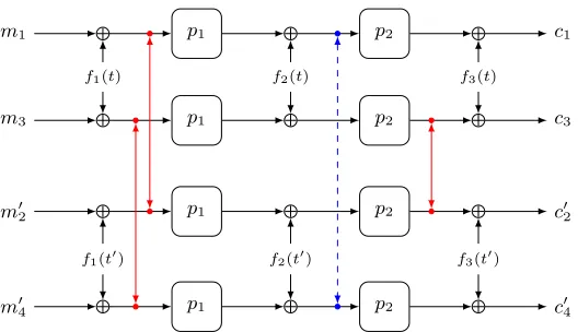
im-plicit throughout). GCLf1,f2,f3 is depicted in Figure 1. If h1, h2 are two XOR universal hash functions, then GCLh1,h1⊕h2,h2 matches CLRW2 (where we set kf = (h1, h2)).
m Ek1 Ek2 c
f1(t) f2(t) f3(t)
Fig. 1: Depiction of GCLf1,f2,f3.
In support of its correctness, the attack is backed up with a formal suc-cess probability computation in Section 3.3 as well as an implementation in Section 3.4. The formal success analysis demonstrates that for n ≥ 27, the distinguisher’s success probability is at least 1/2. The small-scale implemen-tation demonstrates that for GCLf1,f2,f3 based on random permutations on n = 16,20,24 bits, the special collisions as searched for in the attack indeed appear more often than usual. The gap between the accuracy innof the exper-imental verification and the security proof is caused by the fact that some loose probability bounds had to be used in the rather conservative proof.
The attack is independent of the masking functionsf1, f2, f3. It implies that GCLf1,f2,f3 cannot achieve optimal security, regardless of the choice of masking. The attack particularly applies to CLRW2, therewith improving the best known attack to date.
1.2 Towards Tight Security?
In Section 4 we approach the attack from a more theoretical perspective, and describe the main limitations in proving security of GCLf1,f2,f3 beyond 22n/3. The quasi-formal discussion relies on equating executions of GCLf1,f2,f3 with a bipartite graph, and by drawing a parallel with Patarin’s mirror theory [20,22,
26,28] we indicate various issues in trying to prove security beyond 22n/3. The most notable one of these, namely the potential existence of four queries which alternatively collide on the input of Ek1 or output ofEk2 is precisely the one exploited in our attack in 2n1/223n/4 queries. We also pinpoint where and how the current gap between a security lower bound of 22n/3 and an attack upper bound of 23n/4 arises. Most importantly, as the distinguisher can freely choose
the value of the tweak for every query, it can set a certain distinguishing event with a significant probability.
1.3 Improved Security of Cascaded LRW2 Under Tweak Limits
In Section 5 we use these insights obtained in our quest towards tight security. We return to CLRW2, or equivalently GCLh1,h1⊕h2,h2, and prove that if (i)h
condition on the occurrence of the tweak seems restrictive, but many modes of operation based on a tweakable block cipher query their primitives for tweaks that are constituted of a nonce or random number concatenated with a counter value [10,12,15,29]: in a nonce-respecting setting, every nonce appears at most 1 +qf times, where qf is the amount of forgery attempts.
The proof relies on Patarin’s mirror theory up to the first recursion, i.e., up to 3n/4-bit security. It shares ideas with the analysis of Mennink and Neves [20] on Encrypted Davies-Meyer [7], namely that an evaluation (t, m, c) of CLRW2 can be rewritten as a sum of permutations “in the middle.” Adversarial power to choose tweak values, however, precludes optimal security, and security up to 23n/4 is the best possible bound.
1.4 Longer Cascades?
Lampe and Seurin [16] suggested the cascade ofρ≥1 evaluations of LRW2, and proved that for evenρthis construction is secure up to approximately 2ρn/(ρ+2) queries. Lee et al. [18] proved that if the universal hash functions are replaced by random functions, security up to 2ρn/(ρ+1)is achieved. It is generally conjectured that the security of the cascade ofρLRW2’s is 2ρn/(ρ+1)[16–18], but also for this larger cascade, nothing is known on the attack side, besides the trivial attack in 2n queries. Unfortunately, it does not seem possible to generalize the attack
of Section 3nor the security proof of Section 5to larger cascades. As before, it is noteworthy that a cascade of ρ≥1 evaluations of TEM can be attacked in approximately 2ρn/(ρ+1)queries [2].
2
Preliminaries
For n∈ N, {0,1}n denotes the set of bit strings of length n, and perm(n) the set of all permutations on {0,1}n. Extending notation, for κ ∈
N, we denote by iperm(κ, n) the set of all “indexed permutations,” families of permutations pk ∈perm(n), indexed byk∈ {0,1}κ. We additionally denote by iperm(κ, τ, n)
for τ ∈ Nthe set of all indexed permutations where the index consists of two elements (k, t) ∈ {0,1}κ× {0,1}τ. Form, n ∈
Nsuch that m≥ n, the falling factorial is defined as (m)n =m(m−1)· · ·(m−n+ 1) =m!/(m−n)!. Forn∈N andm∈ {0, . . . ,2n−1}, we denote byhmi
n the encoding ofmas ann-bit string.
IfX is a finite set,x←− X$ denotes the event of uniformly randomly drawingx fromX.
2.1 Block Ciphers and Tweakable Block Ciphers
A block cipher with key size κ and state size n is a functionE ∈ iperm(κ, n). For fixed key k∈ {0,1}κ we denote E
k(·) =E(k,·), and its inverse is denoted
Ek−1(·). A tweakable block cipher with key size κ, tweak size τ, and state size n is a functionEe ∈iperm(κ, τ, n). For fixed key k∈ {0,1}κ andt ∈ {0,1}τ we
Letκ, n ∈ N and letE ∈ iperm(κ, n) be a block cipher. The advantage of a distinguisher D in breaking the SPRP (strong pseudorandom permutation) security ofE is defined as
AdvsprpE (D) =PrDEk± = 1−PrDp± = 1, (3)
where the probabilities are taken over the random drawing of k ←− {$ 0,1}κ,
p ←−$ perm(n), and the randomness used by D. The resources that D may use are typically expressed in terms of query complexity (to the oracle) and time complexity (for offline computations).
As block ciphers are a special case of tweakable block ciphers with tweak space of size 1 (τ = 0), the security definition straightforwardly generalizes to the latter. Letκ, τ, n∈Nand letEe∈iperm(κ, τ, n) be a tweakable block cipher.
The advantage of a distinguisher Din breaking the STPRP (strong tweakable pseudorandom permutation) security ofEe is defined as
Advstprp e
E (D) =Pr
DEe±k = 1
−PrDep
±
= 1, (4)
where the probabilities are taken over the random drawing of k ←− {$ 0,1}κ,
e
p←−$ iperm(τ, n), and the randomness used byD. The resources thatDmay use are typically bounded as before.
2.2 XOR Universal Hash Functions
We use the notion of`-wise independent XOR universal hash functions, a slight adaptation of the original definition of Wegman and Carter [34]. For two non-empty sets X,Y, a hash function family H = {h : X → Y} is called `-wise independent almost XOR universal up to boundε, denotedε-AXU`, if for anyj∈
{2, . . . , `}, any distinctx1, . . . , xj∈ X and (not necessarily distinct)y2, . . . , yj ∈
Y,
Prh←−$ H : h(x1)⊕h(x2) =y2, . . . , h(x1)⊕h(xj) =yj
≤εj−1.
For X =Y ={0,1}n, a 2−n-AXU
2 hash function family can be defined using finite field multiplication with respect to some irreducible polynomial to repre-sent the field, i.e., h(x) :=h⊗x. It is notε-AXU` for` >2. Defining the hash
function family as
h(x) :=
`−1
M
i=1 hi⊗xi
forh= (h1, . . . , h`−1) gives a 2−n-AXU`hash function family for any`≥2. One
can alternatively obtain a (2n−(`−1))−1-AXU
` by defining the hash function
3
Generic Attack
We present a generic attack against GCLf1,f2,f3in 2n1/223n/4queries. The attack is generic in nature, it does not exploit any weaknesses in the underlying cipher, and as such we simply assume that E ←−$ iperm(κ, n) is an ideal cipher. It is fair to assume that the success probability of the attack simply improves if E is less than ideal, except for degenerate cases, e.g., if Ek1 and Ek2 are almost perfect nonlinear permutations (APNPs, cf., [8,23,24]). Throughout the attack, we simply denotep1=Ek1 andp2=Ek2 for brevity.
An informal rationale of our attack is given in Section3.1, and the formal distinguisher in Section 3.2. Its advantage is lower bounded in Section3.3, and the analysis is backed up with experimental verification in Section3.4.
3.1 Informal Rationale of Attack
Suppose a distinguisher obtains four queries (t, m1, c1), (t0, m20, c02), (t, m3, c3), and (t0, m04, c40) of GCLf1,f2,f3 such that
m1⊕f1(t) =m02⊕f1(t0), c02⊕f3(t0) =c3⊕f3(t), m3⊕f1(t) =m04⊕f1(t0).
(5)
In other words, the first and second query collide at the input toEk1, the second and third at the output of Ek2, and the third and fourth at the input to Ek1. As the four queries are performed using only two tweak values, each occurring twice, we have f2(t)⊕f2(t0)⊕f2(t)⊕f2(t0) = 0, and from a simple inspection of the scheme (see also Figure2) one can conclude that, necessarily,
c1⊕f3(t) =c40 ⊕f3(t0). (6)
Stated differently, under the assumption that (5) is satisfied, (6) is implied, and therefore the four equations combine to
m1⊕m02=m3⊕m04=f1(t)⊕f1(t0), c02⊕c3=c1⊕c04=f3(t)⊕f3(t0).
Unfortunately, the distinguisher does not know f1(t)⊕f1(t0) andf3(t)⊕f3(t0), but if we ignore these two values in above equations, we obtain
m1⊕m02=m3⊕m04, c02⊕c3=c1⊕c04,
(7)
whichnecessarily holds ifm1⊕m02=f1(t)⊕f1(t0) andc02⊕c3=f3(t)⊕f3(t0), but may hold by accident as well. Stated differently, if for some d ∈ {0,1}n,
there are about 2n choices for the four queries such that
m1
m3
m02
m04
p1
p1
p1
p1
p2
p2
p2
p2
c1
c3
c02
c04
f1(t)
f1(t0)
f2(t)
f2(t0)
f3(t)
f3(t0)
Fig. 2: Attack idea: the red (solid) collisions are targeted, the blue (dashed) one is implied by the red ones.
the expected number of solutions to (7) is close to 2 if d =f1(t)⊕f1(t0) but close to 1 ifd6=f1(t)⊕f1(t0). For an ideal permutation, the expected number of solutions is always close to 1 for any d∈ {0,1}n. By making approximately
23n/4 queries, the distinguisher can ensure that there are about 2n solutions to
(8) for all d, includingd=f1(t)⊕f1(t0).
This almost allows for a distinguishing attack, but not quite: as the distin-guisher does not actually knowf1(t)⊕f1(t0), it must simply hope that for some d there is a significant difference, butdmay take 2n values and false positives
are likely to occur. By extending the number of queries slightly, i.e., by making aboutn1/2·23n/4 queries, the case off1(t)⊕f1(t0) will stand out.
We remark that the attack is effectively an XOR subkey recovery attack, as the distinguisher learnsf1(t)⊕f1(t0) and f3(t)⊕f3(t0). In case of Cascaded LRW2, where f1 =h1, f2 =h1⊕h2, andf3=h2 for two XOR universal hash functions h1, h2, this immediately gives f2(t)⊕f2(t0), and potentially more, depending on the specific hash functions.
3.2 Formal Description of Distinguisher
Let = log2(n)/2 (assumed to be integral), and consider the following distin-guisherDmakingq= 23n/4+queries.
(i) Fix arbitrary distinctt, t0 ∈ {0,1}τ;
(ii) Fori= 0, . . . ,23n/4+−1, putm
i = 0n/4−khii3n/4+ and query (t, mi) to
obtainci;
(iii) Fori= 0, . . . ,23n/4+−1, putm0
i=hii3n/4+k0n/4−and query (t0, m0i) to
obtainc0i;
(iv) Ford∈ {0,1}n, defineI
d={(i, j)|mi⊕mj0 =d}. Note that|Id|= 2n/2+2
for alld∈ {0,1}n, and defineq0 := 2n/2+2;
– DefineNd= 0;
– For all distinct (i, j),(k, l)∈Id: ifci⊕c0l=c0j⊕ck, putNd =Nd+ 1;
(vi) Briefly looking forward, for a random tweakable block cipher we have
Ex(Nd) = q
0 2
/(2n −1) for any d ∈ {0,1}n, whereas for GCLf1,f2,f3,
Ex Nf1(t)⊕f1(t0)
≥2 q20
/2n. Inspired by this, define
β := 3 2
q0
2
/2n.
If there exists ad∈ {0,1}n such thatN
d≥β, output 1. Otherwise, output
0.
3.3 Analysis of Distinguisher Advantage
A formal analysis confirms that the distinguisher succeeds with non-negligible probability.
Theorem 1. Let κ, τ, n ∈ N with n ≥ 16, let E ←−$ iperm(κ, n), denote the
size of the key space of (f1, f2, f3) byκf, and consider GCLf1,f2,f3 :{0,1}2κ×
{0,1}κf× {0,1}τ× {0,1}n → {0,1}n. DistinguisherDof Section3.2with query
complexity 2n1/2·23n/4 has advantage
AdvstprpGCLf1,f2,f3(D)≥1− 32 n2 −
80
n2n/2 −5·2
n
10
n
3/100·n2
− n
7
23n/2. (9)
One can verify that the lower bound of (9) is at least 1/2 for n ≥ 27. This theorem is not the core contribution of the article (which is Theorem2), and its proof is given AppendixA.
Note that the attack is de facto a TPRP-attack, only requiring forward ac-cess to the scheme. In addition, it is information-theoretical: the distinguisher’s complexity is solely measured in its number of queries. The offline complexity is around 23n/2.
3.4 Experimental Verification
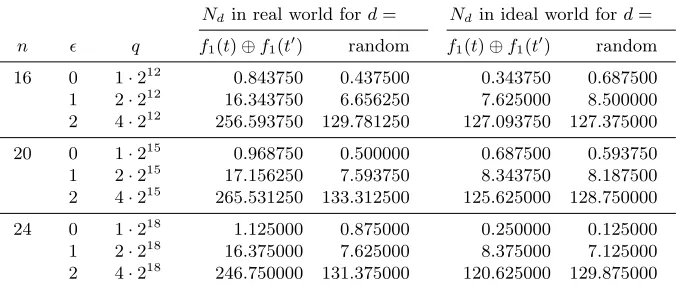
We have implemented the distinguisher of Section 3.2 on a small scale, for n= 16,20,24 and withp1, p2, f1, f2, f3instantiated as independent uniform ran-dom permutations, noting that a uniform ranran-dom permutation is a (2n−1)−1 -AXU2hash function (see Section2.2). In each case, two distinct tweakst, t0 are evaluated for q= 23n/4+ queries, with = 0,1,2 (note that 2
.log2(n)/2 for n= 16,20,24). The average valuesNdfor both the real and ideal world and both
Table 1: Number of elements inNd for the real and ideal world, ford=f1(t)⊕
f1(t0) and for randomd. For the casesn= 16,20, the numbers are averaged over 32 attacks; forn= 24 the numbers are averaged over 8 attacks.
Ndin real world ford= Ndin ideal world ford= n q f1(t)⊕f1(t0) random f1(t)⊕f1(t0) random
16 0 1·212 0.843750 0.437500 0.343750 0.687500 1 2·212 16.343750 6.656250 7.625000 8.500000 2 4·212 256.593750 129.781250 127.093750 127.375000 20 0 1·215 0.968750 0.500000 0.687500 0.593750
1 2·215 17.156250 7.593750 8.343750 8.187500 2 4·215 265.531250 133.312500 125.625000 128.750000
24 0 1·218 1.125000 0.875000 0.250000 0.125000
1 2·218 16.375000 7.625000 8.375000 7.125000 2 4·218 246.750000 131.375000 120.625000 129.875000
case (real or ideal world), and the statistics in Table 1 reasonably accurately match these numbers.
Note that, in particular, for = 0 the value Nf1(t)⊕f1(t0) already shows a small peak in the real world (for each of n= 16,20,24), but outliers in Nd for
d6=f1(t)⊕f1(t0) are hidden by the statistics. For increasing, the gap becomes more significant and the success probability increases.
4
Towards Tight Security?
Consider a simplification of GCLf1,f2,f3 with its two block ciphers replaced by random permutationsp1, p2(this is a typical hybrid argument in security proofs performed at the cost of 2AdvsprpE (D0) for some distinguisherD0). For simplicity, assume thatf2is injective (the scheme turns out to be significantly weakened if f2 is non-injective). For an evaluation GCLf1,f2,f3(t, m) =c, denote
x=p1(m⊕f1(t)),
y=p−21(c⊕f3(t)),
in such a way thatx⊕y=f2(t).
Intuitively, one may think of a proof going “fine” if there is always some randomness available. For example, consider just a single forward query (t, m) to GCLf1,f2,f3. The value m⊕f1(t) has never been evaluated by p1, hence the value xwill look uniformly randomly drawn from {0,1}n; the value y satisfies
y =x⊕f2(t), and alsoy has never been evaluated by p2 so the value c⊕f3(t) is uniformly randomly drawn from{0,1}n.
before, rendering freshx1andc1⊕f3(t1). The second query satisfiesm1⊕f1(t1) = m2⊕f1(t2), meaning that x2 =x1. However, as the two queries are distinct, this equation implies that t1 6= t2. As f2 is injective, we subsequently have f2(t1) 6= f2(t2) and thus y2 6= y1. The evaluation of p2 on y2 yields a value uniformly drawn from{0,1}n\{c1⊕f3(t1)}.
Likewise, two queries could also collide at the right side, i.e.,c1⊕f3(t1) = c2⊕f3(t2). It is unlikely, though, that two queries collide atboth the left and right side, at least if f1 and f3 are two randomized functions (as is the case in CLRW2), and we will ignore this case. If more than two queries are involved, one could visualize queries as a bipartite graph G = (U, V, E). U = {0,1}n
corresponds to the input values to p1,V ={0,1}n to the output values of p2,
and for every query tuple (ti, mi, ci), the edge (mi⊕f1(ti), ci⊕f3(ti)) with label
f2(ti) fromU toV is added toE. An example graphGis depicted in Figure3.
¯
m1 m¯2= ¯m3 m¯4= ¯m5= ¯m6 m¯7
¯
c1 ¯c2 ¯c3 c¯4 ¯c5 ¯c6= ¯c7
f2(t1) f2(t2)f2(t3) f2(t4)
f2(t5)
f2(t6) f2(t7)
Fig. 3: Example of a bipartite graph G representing seven evaluations of GCLf1,f2,f3. For brevity, we denote ¯m
i = mi⊕f1(ti) and ¯ci = ci ⊕f3(ti).
Graph view rotated for economical reasons.
What the above comprises is an informal introduction to a potential use of Patarin’s mirror theory [20,22,26,28], a powerful approach towards counting the number of solutions to a system of equations of the form x⊕y =λ, where λ is known. If, in above graph, two queries touch on the left, i.e.,m1⊕f1(t1) = m2⊕f1(t2), they share the samex1=x2but have differenty1, y2.
Unfortunately, the mirror theory does not turn out to be particularly suited here, most importantly as it is tailored towards comparing systems to random functions and we aim to compare our scheme to a family of permutations. Yet, closer inspection of the theory reveals that it puts two conditions on the graph that are “reasonably easily” violated:
(i) The graph should not contain a path of even length whose labels sum to 0; (ii) The graph should not contain a circle.
The attack of Section3 relies on the fact that condition (i) can be violated easier than expected. Note that there cannot exist a path of length 2 whose labels sum to 0 (as f2 is injective). A path of length 4 whose labels sum to 0 requires the existence of four queries (t1, m1, c1), . . . ,(t4, m4, c4) such that
m1⊕f1(t1) =m2⊕f1(t2), c2⊕f3(t2) =c3⊕f3(t3), m3⊕f1(t3) =m4⊕f1(t4), f2(t1)⊕f2(t2)⊕f2(t3)⊕f2(t4) = 0.
(10)
As the four queries are distinct, the path may only appear ift16=t2 6=t36=t4. However, it may be that t1 = t3 and t2 = t4, and this is how the attack of Section3exploits a path: in this case, the fourth equation of (10) is satisfied by design and the remaining three can be rewritten as
m1⊕m2=m3⊕m4=f1(t1)⊕f1(t2), c2⊕c3=f3(t1)⊕f3(t2).
(11)
The attack of Section3relies on the additional fact that if these conditions are met, then the condition
c4⊕f3(t2) =c1⊕f3(t1) (12)
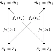
holds with probability 1 in the real world (i.e., there is a circle as depicted in Figure 4, violating condition (ii)), but with negligible probability in the ideal world. This property (that (11) implies (12)) gives a clean and well-verifiable distinguishing event.
¯
m1= ¯m2 m¯3= ¯m4
¯
c1= ¯c4 ¯c2= ¯c3
f2(t1)
f2(t2)
f2(t3)
f2(t4)
Fig. 4: A circle in bipartite graphGwithf2(t1)⊕f2(t2)⊕f2(t3)⊕f2(t4) = 0, as exploited in the attack of Section3. We use the same convention as in Figure3.
A distinguisher can choose the mi’s smartly to make sure thatm1⊕m2 = m3⊕m4is satisfied. Consider a distinguisher that makes queries for at most two tweakst, t0, each queriedqtimes, say for queries (m0, c0), . . . ,(mq−1, cq−1) and (m00, c00), . . . ,(m0q−1, c0q−1). Inspired by Section3, denote
The probability that there exist four queries (i, j)6= (i0, j0) that comply with the equations of (11), denotedX, is
Pr(X) = X
d∈{0,1}n
Pr(X |f1(t1)⊕f1(t2) =d)·Pr(f1(t1)⊕f1(t2) =d)
≈ X
d∈{0,1}n |Id|
2
2n ·Pr(f1(t1)⊕f1(t2) =d)
≈ X
d∈{0,1}n |Id|
2
2n ·
1
2n, (13)
where the first approximation assumes independence of events and that theci’s
are generated using a random function (for simplicity of reasoning), and the second approximation assumes that f1 is close to a 2−n-AXU2 hash function. The two extremes in selecting themi’s are the following:
– Choose themi’s andm0i’s such that |Id|=q forq values of dand |Id| = 0
for the remaining 2n−q values. This is achieved by setting mi = m0i =
0n−log2(q)khii
log2(q)fori= 0, . . . , q−1. In this case, we obtain for (13):
(13) =q·
q 2
/22n≈q3/22n;
– Choose themi’s andm0i’s such that|Id|=q2/2n for all values ofd, i.e.,Id is
equally large for alld. This is achieved by setting mi = 0n−log2(q)khiilog 2(q) and m0i = hiilog2(q)k0n−log2(q) for i = 0, . . . , q−1 (as in the attack of Sec-tion3). In this case, we obtain for (13):
(13) = 2n·
q2/2n
2
/22n≈q4/23n.
A security analysis, i.e., an upper bound on the distinguisher’s success probabil-ity, would have to take into account any possible distinguisher, and it therefore seems such analysis caps at aroundq3/22n. Yet, if the attack of Section3would
have been based on the former strategy instead of the latter, it would have suc-ceeded only if |If1(t1)⊕f1(t2)| 6= 0, and the attack should have been evaluated 2n/q times to succeed (resulting in total complexity of about 2n). By making 23n/4 queries, the distinguisher makes sure that|Id| is equally large for all d’s
and that way spreads its chances, but unfortunately, we see little opportunities in improving the attack.
It is important to remark that the attack of Section 3 and the discussion on the distinguishing event (11) consider the case where the distinguisher can
choose the tweak values. This implies that an improved security bound can be achieved if the maximum number of queries for each tweak is fixed.
and we cannot draw any formal conclusion from it. However, even for this limited scenario, improved security of CLRW2 is still a non-trivial open problem. We elaborate on the possibility of releasing the tweak usage limitation in Section5.7.
A final condition that the mirror theory puts on the graph, in addition to (i) and (ii) above, is the following:
(iii) The graph should not contain an excessively large tree.
This is a merely technical requirement to make the proof argument of the mirror theory work, and it is not clear how a violation of condition (iii) may break the scheme. That said, also condition (iii) can be easily violated, depending on the mixing functions in use. For example, iff1(t) =f1⊗t (i.e., the example AXU2 hash function of Section2), a collision of the form
m1⊕f1(m1) =m2⊕f1(m2),
form1, m26= 0 implies that also
m2⊕f1(m2) =m−11m 2
2⊕f1(m−11m 2
2) =· · ·=m −λ
1 m
λ+1
2 ⊕f1(m−1λm
λ+1 2 ),
for any λ≥0, potentially rendering an excessively large tree. The issue can be resolved by resorting to 4-wise independent XOR universal hash functions (see Section2.2).
5
Improved Security of Cascaded LRW2 Under Tweak
Limits
Based on the two conclusions from Section 4, we prove that if h1 and h2 are two 4-wise independent XOR universal hash functions and every tweak occurs at most q1/3 times, the Cascaded LRW2 construction GCLh1,h1⊕h2,h2 of (2) achieves security up to complexity approximately 23n/4.
Theorem 2. Let κ, τ, n∈N, letE ∈iperm(κ, n),H be an ε-AXU4 hash
func-tion family, and consider GCLh1,h1⊕h2,h2 :{0,1}2κ×H2× {0,1}τ× {0,1}n →
{0,1}n. Letγ ∈
Nsuch that 2≤γ≤q/4 be a threshold. For any distinguisher
Dwith query complexity at most q≤2n/1600that queries each tweak at mostγ
times, there exists a distinguisherD0 that makes at most q queries such that
AdvstprpGCLh1,h1⊕h2,h2(D)≤6
q
4
2nε4+
q
2
(2γ+ 1)ε2+(γ+ 3)q
2n + 2Adv
sprp
E (D
0).
(14)
The proof of Theorem 2 is based on Patarin’s mirror theory [22,26,28], which found popularization in the work of Mennink and Neves on Encrypted Davies-Meyer and its dual [20]. Although the mirror theory is quite simple to understand and apply, its proof is heavy and the recursive argument underneath it is debated by some. In this work, however, we will only use the mirror theory up to 3n/4-bit security, i.e., rely on the first recursion in the mirror theory proof only.
The security proof is comparable to that of EDM [20], and in particular also relies on the observation that any evaluation of c= GCLh1,h1⊕h2,h2(k, t, m) for
k= (k1, k2, h1, h2) can be rewritten as
Ek1(m⊕h1(t))⊕E −1
k2(c⊕h2(t)) =h1(t)⊕h2(t). (15)
Differences in the analysis occur due to the possibility of the adversary to choose the tweak and the fact that the tweak occurs in all three parts of the equation (input to Ek1, toE
−1
k2, and in the right hand side h1(t)⊕h2(t)). These differ-ences cause that only security up to 23n/4is achievable. However, the differences compared with the analysis in [20] mostly affect description of oracle views and analysis of bad views; the application of the mirror theory is fairly the same. Therefore, we discard much of the details on mirror theory from the proof and include it in AppendixB; the proof is fully intelligible without this appendix.
The proof is given in Sections5.1-5.6. We discuss the possibility of releasing the limitationγon the tweak usage in Section5.7.
5.1 H-Coefficient Technique
We will use Patarin’s H-coefficient technique [25,27], for which we follow the de-scription by Chen and Steinberger [5]. Consider two oraclesOandP with iden-tical interfaces, and a deterministic distinguisherDwith query complexityqand unbounded computational power that tries to distinguish both oracles. Denote its success probability by∆D(O;P). LetXOdenote the probability distribution of views whenDis interacting withO, and similarlyXP the distribution of views for interaction withP. A viewν is called “attainable” ifPr(XP =ν)>0, and denote by V the set of all attainable views. The H-coefficient technique states the following:
Lemma 1 (H-coefficient technique).LetDbe a deterministic distinguisher, and consider a partition V = Vbad∪ Vgood of the set of attainable views. Let
δ, ∈[0,1]be such that Pr(XP ∈ Vbad)≤δ, and
Pr(XO =ν)
Pr(XP =ν)
≥1−for all
ν ∈ Vgood. Then, the distinguishing advantage satisfies∆D(O;P)≤δ+.
A proof of the technique is given among others in [4,5,20].
For viewν ={(x1, y1), . . . ,(xq, yq)} consisting ofq input/output tuples, an
5.2 General Setting and Views
Let pe←−$ iperm(τ, n), k ←− {$ 0,1}2κ×H2, and p1, p2 $
←− perm(n). Consider any distinguisherDwhose goal is to distinguish GCLh1,h1⊕h2,h2
k from ep.
As a first step, we replace (Ek1, Ek2) by (p1, p −1
2 ) at the cost of 2Adv sprp
E (D
0), whereD0is some distinguisher with the same query complexityqasD. (Note that we replaced Ek2 bythe inverse ofp2 for simplicity of further analysis.) Denote the resulting scheme withF for brevity; it remains to bound the advantage ofD
in distinguishingO=F(the real world) fromP =pe(the ideal world). As of now, we give the distinguisher unbounded computational power, and its complexity will only be measured by the number of oracle queries it makes. Without loss of generality, we can consider it to be deterministic, and will apply the H-coefficient technique of Lemma1.
Dmakesqconstruction queries which are recorded in viewν0={(t1, m1, c1), . . . ,(tq, mq, cq)}. AfterD’s interaction with its oracle, but before it outputs its
decision bit, its oracle will reveal the subkeysh1, h2. In the real world, these are the XOR universal hash functions used in F, whereas in the ideal world these are dummy functions randomly drawn fromH. We denote the complete view by
ν = (ν0, h1, h2). (16)
Without loss of generality, we assume thatD never repeats queries, and hence that (ti, mi)6= (tj, mj) and (ti, ci)6= (tj, cj) for anyi6=j.
5.3 Attainable Index Mappings
In the real worldO, each tuple (ti, mi, ci)∈ν0 corresponds to an evaluation of
F and satisfies
p1(mi⊕h1(ti))⊕p2(ci⊕h2(ti)) =h1(ti)⊕h2(ti),
where we recall thatEk2 was replaced withp −1
2 . WritingPai :=p1(mi⊕h1(ti)) andPbi :=p2(ci⊕h2(ti)), viewν defines the followingqequations:
Pa1⊕Pb1=h1(t1)⊕h2(t1), Pa2⊕Pb2=h1(t2)⊕h2(t2),
.. .
Paq⊕Pbq=h1(tq)⊕h2(tq).
(17)
Here, some of the unknowns may be equal to each other. We have thatPai 6=Paj if and only ifmi⊕h1(ti)6=mj⊕h1(tj), andPbi 6=Pbj if and only ifci⊕h2(ti)6= cj⊕h2(tj). No condition a priori holds forPai versusPbj, as these are defined by independent permutations. We have
r=|{mi⊕h1(ti)|i∈ {1, . . . , q}}|+|{ci⊕h2(ti)|i∈ {1, . . . , q}}| (18)
5.4 Bad Views
Inspired by the discussion in Section4, we associate a bipartite graphG(ν) = (U, V, E(ν)) with the viewν.U ={0,1}n corresponds to the input values to p
1, V ={0,1}n to the output values ofp−1
2 , and for every (ti, mi, ci)∈ν0, the edge
(mi⊕h1(ti), ci⊕h2(ti)) with labelh1(ti)⊕h2(ti) fromU toV is added toE(ν).
The example graph of Figure 3 still applies, be it with f1 =h1, f2 =h1⊕h2, andf3=h2.
In Section4, we already informally discussed what problems could occur in such a graph, i.e., what properties would make the mirror theory inapplicable: it should not contain a path of even length whose labels sum to 0, a circle, or an excessively large tree. The latter is informal, it is often based on a pre-defined threshold on the maximum size of the tree. As our security analysis will cap on 3n/4-bit security anyway, we can keep it simple, and put as one of the bad events that G(ν) should not contain a subgraph of ≥ 4 edges. This would imply the non-existence of an excessively large tree, as well as circles and paths of length
≥4. We still have to rule out the existence of a path of length 2 whose labels sum to 0 and a circle of length 2.
Formally, we say that a viewν is a bad view if its corresponding tree G(ν) contains
(i) a path of length 2 whose labels sum to 0; (ii) a circle of length 2;
(iii) a subgraph of≥4 edges.
5.5 Probability of Bad Views (δ)
By Lemma 1, we have to analyze the probability that a view generated in the ideal world is bad, and the analysis will rely on the fact thath1andh2are 4-wise independent universal hash functions. We have
Pr(X
e
p∈ Vbad)≤Pr(path) +Pr(circle) +Pr(subgraph), (19) where the sizes of the path, circle, and subgraph, are left implicit.
(i) a path. Consider any two distinct queries (ti, mi, ci),(tj, mj, cj). They yield
a 0-label-sum path if either
mi⊕h1(ti) =mj⊕h1(tj) andh1(ti)⊕h2(ti) =h1(tj)⊕h2(tj),
or
ci⊕h2(ti) =cj⊕h2(tj) andh1(ti)⊕h2(ti) =h1(tj)⊕h2(tj).
Ifti=tj, then necessarilymi=6 mj andci6=cj (as the two queries are distinct)
and the conditions happen with probability 0. Otherwise, as h1 and h2 are ε -AXU4, both conditions happen with probability at mostε2. Thus,
Pr(path)≤2
q
2
(ii) a circle. Consider any two distinct queries (ti, mi, ci),(tj, mj, cj). They yield
a circle if
mi⊕h1(ti) =mj⊕h1(tj) andci⊕h2(ti) =cj⊕h2(tj),
which, as before, happens with probability at mostε2. Thus,
Pr(circle)≤
q
2
ε2. (21)
(iii) a subgraph. Consider any four distinct queries (ti1, mi1, ci1), . . . , (ti4, mi4, ci4) to yield a subgraph. We can consider six possible configurations, as described in Figure5. In these configurations, only collisions are explicitly indi-cated; two nodes that are different in the configuration may or may not collide. We treat all configurations independently, where we will rely on the fact thath1 andh2 areε-AXU4.
(A) (B) (C) (D) (E) (F)
Fig. 5: Possible configurations of subgraphs of 4 edges. Upper shore isU, lower shore isV, and labels are omitted for brevity. Two nodes in the same shore may or may not be equal.
(A) Configuration (A) happens only if
mi1⊕h1(ti1) =mi2⊕h1(ti2) =mi3⊕h1(ti3) =mi4⊕h1(ti4).
If the tweaks are not all distinct, the condition is satisfied with probability 0. On the other hand, ifti1, ti2, ti3, ti4 are all distinct, the condition is satisfied with probability at mostε3. There are at most q4possible choices of queries that satisfy this condition on the tweaks;
(B) Configuration (B) happens only if
mi1⊕h1(ti1) =mi2⊕h1(ti2) =mi3⊕h1(ti3), ci3⊕h2(ti3) =ci4⊕h2(ti4).
Further analysis depends on the values of the tweaks.
– Ifti1, ti2, ti3, ti4are all distinct, the condition is satisfied with probability at mostε3. There are at most q
4
– If ti1 =ti2, ti1 =ti3, ti2 = ti3, or ti3 =ti4, the condition is satisfied with probability 0;
– Ifti1 =ti4, butti1, ti2, ti3 are all distinct, the condition is satisfied with probability at mostε3. There are at most q
3
·(γ−1) possible choices of queries that satisfy this condition on the tweaks, noting that every tweak occurs at mostγ times;
– Ifti2 =ti4, butti1, ti2, ti3 are all distinct, a similar reasoning applies. Overall, configuration (B) is satisfied with probability at most
max
q 4
ε3,
q 3
(γ−1)ε3
≤
q 4
ε3,
forγ≤q/4;
(C) Configuration (C) happens only if
mi1⊕h1(ti1) =mi2⊕h1(ti2), ci2⊕h2(ti2) =ci3⊕h2(ti3), mi3⊕h1(ti3) =mi4⊕h1(ti4).
Further analysis depends on the values of the tweaks.
– If ti1, ti2, ti3, ti4 are all distinct, the condition is satisfied with proba-bility at most 2nε4 (obtained by summing over all possible connections between the first and third equation, and then applying the ε-AXU4 bound). There are at most q4
possible choices of queries that satisfy this condition on the tweaks;
– If ti1 =ti2,ti2 =ti3, orti3 =ti4, the condition is satisfied with proba-bility 0;
– Ifti1 =ti3, butti1, ti2, ti4 are all distinct, the condition is satisfied with probability at mostε3. There are at most q
3
·(γ−1) possible choices of queries that satisfy this condition on the tweaks, noting that every tweak occurs at mostγ times;
– Ifti2 =ti4, butti1, ti2, ti3 are all distinct, a similar reasoning applies;
– Ifti1 =ti4, butti1, ti2, ti3 are all distinct, a similar reasoning applies;
– Ifti1 =ti3 andti2=ti4 butti1, ti2are distinct, the condition is satisfied with probability at most ε2. There are at most q
2
·(γ−1) possible choices of queries that satisfy this condition on the tweaks, noting that every tweak occurs at mostγtimes and that there is at most one option for (ti4, mi4, ci4) once the other three queries are fixed.
Overall, configuration (C) is satisfied with probability at most
max
q
4
2nε4,
q
3
(γ−1)ε3,
q
2
(γ−1)ε2
≤
q
4
2nε4+
q
2
(γ−1)ε2,
forγ≤q/4 and 2nε≥1;
Thus,
Pr(subgraph)≤4
q
4
ε3+ 2
q
4
2nε4+ 2
q
2
(γ−1)ε2
≤6
q
4
2nε4+ 2
q
2
(γ−1)ε2. (22)
Conclusion for bad events. From (19) and the individual probabilities of (20), (21), and (22), we obtain
Pr(X
e
p∈ Vbad)≤3
q
2
ε2+ 6
q
4
2nε4+ 2
q
2
(γ−1)ε2
≤6
q
4
2nε4+
q
2
(2γ+ 1)ε2,
forγ≥2.
5.6 Ratio for Good Views ()
Consider a given viewν = (ν0, h1, h2) where ν ={(t1, m1, c1), . . . ,(tq, mq, cq)}.
Define
r1=|{mi⊕h1(ti)|i∈ {1, . . . , q}}|, (23)
r2=|{ci⊕h2(ti)|i∈ {1, . . . , q}}|. (24)
Note thatr1+r2is equal to the number of unknowns in the system of equations (see (18)). For anyt∈ {0,1}τ, we denote u
t=|{i∈ {1, . . . , q} |ti=t}|.
For the ideal worldpe, we have
Pr(X
e
p=ν) =Pr
e
p←−$ iperm(τ, n) : pe`ν0·Pr(h1, h2) = (h01, h02)←−$ H2
= Q 1
t∈{0,1}τ(2n)ut
· 1
|H|2, (25)
where for the first probability we use thatepis a family of permutations and for every t∈ {0,1}τ the view defines u
tvalues.
For the real world F, recall that it is built from two permutations p1, p−21. We have
Pr(XF =ν) =Pr
p1, p−21←−$ perm(n) : F `ν0 |h1, h2·Pr(h1, h2) = (h01, h02)←−$ H2
=Prp1, p−21 $
←−perm(n) : F `ν0 |h1, h2
· 1
|H|2. (26)
Lemma 2. Consider good view ν = (ν0, h1, h2) whose system of q equations
(17) has no subgraph of≥4 edges, has no path of length2 whose labels sum to
0, and no circle of length2. As long as52·q≤2n/64, the number of solutions
to the r1+r2 unknowns is at least
(2n) r1(2
n−4) r2
2nq .
The proof of Lemma 2 is omitted: it is very similar to the reasoning on EDM in [20] and follows straightforwardly from Patarin’s mirror theory as reviewed in AppendixB. The side condition 52·q≤2n/64 is slightly different from that in [20], as we have adopted the bound from Nachef, Patarin, and Volte [22].
Every such solution definesr1evaluations ofp1, andr2evaluations ofp2, and hence the remaining probability in (26) satisfies
Prp1, p−21←−$ perm(n) : F `ν0|h1, h2≥ (2
n) r1(2
n−4) r2 2nq·(2n)
r1(2
n) r2
.
We obtain for the ratio:
Pr(XF =ν) Pr(X
e p=ν)
≥
Q
t∈{0,1}τ(2n)ut· |H| 2
1 ·
(2n)r1(2
n−4) r2 2nq·(2n)
r1(2
n) r2· |H|
2
=
Q
t∈{0,1}τ(2n)ut·(2
n−4) r2 2nq·(2n)
r2
. (27)
Using that for allt,ut≤γ, and thatPt∈{0,1}τut=q:
(27)≥
Q
t∈{0,1}τ(2n−(γ−1))ut·(2n−4)r2 2nq·(2n)
r2
=
2n−(γ−1)
2n
q
·
3
Y
i=0
1− r2
2n−i
. (28)
Using that r2≤q−1, and by simple algebra for q≤2n/3:
(28)≥1−
(γ
−1)q
2n +
q−1 2n +
q−1 2n−1+
q−1 2n−2 +
q−1 2n−3
≥1−(γ+ 3)q
2n .
We have obtained= (γ+3)2n q, provided 5
2·q≤2n/64.
5.7 Releasing Tweak Usage Limitation
The first place is the last case of configuration (C) in Section5.5, namely the case whereti1 =ti3 andti2 =ti4. For upper bounding the number of choices for the four queries without relying on parameterγ, one may take into account that mi1 ⊕mi2 =mi3 ⊕mi4 is necessarily needed. This value needs to be equal to the random valueh1(ti1)⊕h2(ti2). However, we see no possibility for deriving a formal bound here.
The second place is in the application of the mirror theory in Section 5.6. Our approach to achieve improved 3n/4-bit security relies on Patarin’s mirror theory, which is specifically developed to work well if a scheme is compared with a random function. Obviously, evaluations of CLRW2 under the same tweak will always give distinct responses. In particular, if a distinguisher uses the same tweak for all queries, all responses will be distinct, and the scheme can be distin-guished from a random function with probability about q2/2n. More generally, if every tweak is evaluated at mostγtimes, the scheme can be distinguished from a random function with probability at most aroundγq/2n. Resolving theγ
lim-itation here requires improving Patarin’s mirror theory or employing a different proof technique.
Acknowledgments. Bart Mennink is supported by a postdoctoral fellow-ship from the Netherlands Organisation for Scientific Research (NWO) under Veni grant 016.Veni.173.017. The author would like to thank Mridul Nandi and Samuel Neves, and anonymous reviewers for their comments and suggestions.
References
1. Andreeva, E., Bogdanov, A., Luykx, A., Mennink, B., Tischhauser, E., Yasuda, K.: Parallelizable and Authenticated Online Ciphers. In: Sako, K., Sarkar, P. (eds.) ASIACRYPT 2013, Part I. Lecture Notes in Computer Science, vol. 8269, pp. 424–443. Springer (2013)
2. Bogdanov, A., Knudsen, L.R., Leander, G., Standaert, F., Steinberger, J.P., Tis-chhauser, E.: Key-Alternating Ciphers in a Provable Setting: Encryption Using a Small Number of Public Permutations - (Extended Abstract). In: Pointcheval, D., Johansson, T. (eds.) EUROCRYPT 2012. Lecture Notes in Computer Science, vol. 7237, pp. 45–62. Springer (2012)
3. Chakraborty, D., Sarkar, P.: A General Construction of Tweakable Block Ciphers and Different Modes of Operations. In: Lipmaa, H., Yung, M., Lin, D. (eds.) In-scrypt 2006. Lecture Notes in Computer Science, vol. 4318, pp. 88–102. Springer (2006)
4. Chen, S., Lampe, R., Lee, J., Seurin, Y., Steinberger, J.P.: Minimizing the Two-Round Even-Mansour Cipher. In: Garay, J.A., Gennaro, R. (eds.) CRYPTO 2014, Part I. Lecture Notes in Computer Science, vol. 8616, pp. 39–56. Springer (2014) 5. Chen, S., Steinberger, J.P.: Tight Security Bounds for Key-Alternating Ciphers. In:
Nguyen, P.Q., Oswald, E. (eds.) EUROCRYPT 2014. Lecture Notes in Computer Science, vol. 8441, pp. 327–350. Springer (2014)
7. Cogliati, B., Seurin, Y.: EWCDM: An Efficient, Beyond-Birthday Secure, Nonce-Misuse Resistant MAC. In: Robshaw and Katz [31], pp. 121–149
8. Dunkelman, O., Keller, N.: A New Criterion for Nonlinearity of Block Ciphers. IEEE Trans. Information Theory 53(11), 3944–3957 (2007)
9. Dworkin, M.: NIST SP 800-38E: Recommendation for Block Cipher Modes of Op-eration: The XTS-AES Mode for Confidentiality on Storage Devices (2010) 10. Granger, R., Jovanovic, P., Mennink, B., Neves, S.: Improved Masking for
Tweak-able Blockciphers with Applications to Authenticated Encryption. In: Fischlin, M., Coron, J. (eds.) EUROCRYPT 2016, Part I. Lecture Notes in Computer Science, vol. 9665, pp. 263–293. Springer (2016)
11. Hoang, V.T., Krovetz, T., Rogaway, P.: Robust Authenticated-Encryption AEZ and the Problem That It Solves. In: Oswald, E., Fischlin, M. (eds.) EUROCRYPT 2015, Part I. Lecture Notes in Computer Science, vol. 9056, pp. 15–44. Springer (2015)
12. Iwata, T., Minematsu, K., Peyrin, T., Seurin, Y.: ZMAC: A Fast Tweakable Block Cipher Mode for Highly Secure Message Authentication. In: Katz and Shacham [14], pp. 34–65
13. Jean, J., Nikoli´c, I., Peyrin, T., Seurin, Y.: Deoxys v1.41 (2016), submission to CAESAR competition
14. Katz, J., Shacham, H. (eds.): CRYPTO 2017, Part III, Lecture Notes in Computer Science, vol. 10403. Springer (2017)
15. Krovetz, T., Rogaway, P.: The Software Performance of Authenticated-Encryption Modes. In: Joux, A. (ed.) FSE 2011. Lecture Notes in Computer Science, vol. 6733, pp. 306–327. Springer (2011)
16. Lampe, R., Seurin, Y.: Tweakable Blockciphers with Asymptotically Optimal Se-curity. In: Moriai, S. (ed.) FSE 2013. Lecture Notes in Computer Science, vol. 8424, pp. 133–151. Springer (2013)
17. Landecker, W., Shrimpton, T., Terashima, R.S.: Tweakable Blockciphers with Be-yond Birthday-Bound Security. In: Safavi-Naini, R., Canetti, R. (eds.) CRYPTO 2012. Lecture Notes in Computer Science, vol. 7417, pp. 14–30. Springer (2012) 18. Lee, J., Luykx, A., Mennink, B., Minematsu, K.: Connecting Tweakable and
Multi-Key Blockcipher Security. Des. Codes Cryptography 86(3), 623–640 (2018) 19. Liskov, M., Rivest, R.L., Wagner, D.A.: Tweakable Block Ciphers. In: Yung, M.
(ed.) CRYPTO 2002. Lecture Notes in Computer Science, vol. 2442, pp. 31–46. Springer (2002)
20. Mennink, B., Neves, S.: Encrypted Davies-Meyer and Its Dual: Towards Optimal Security Using Mirror Theory. In: Katz and Shacham [14], pp. 556–583
21. Minematsu, K.: Improved Security Analysis of XEX and LRW Modes. In: Biham, E., Youssef, A.M. (eds.) SAC 2006. Lecture Notes in Computer Science, vol. 4356, pp. 96–113. Springer (2006)
22. Nachef, V., Patarin, J., Volte, E.: Feistel Ciphers - Security Proofs and Cryptanal-ysis. Springer (2017)
23. Nyberg, K.: Perfect Nonlinear S-Boxes. In: Davies, D.W. (ed.) EUROCRYPT ’91. Lecture Notes in Computer Science, vol. 547, pp. 378–386. Springer (1991) 24. Nyberg, K., Knudsen, L.R.: Provable Security Against Differential Cryptanalysis.
In: Brickell, E.F. (ed.) CRYPTO ’92. Lecture Notes in Computer Science, vol. 740, pp. 566–574. Springer (1992)
26. Patarin, J.: On Linear Systems of Equations with Distinct Variables and Small Block Size. In: Won, D., Kim, S. (eds.) ICISC 2005. Lecture Notes in Computer Science, vol. 3935, pp. 299–321. Springer (2005)
27. Patarin, J.: The “Coefficients H” Technique. In: Avanzi, R.M., Keliher, L., Sica, F. (eds.) SAC 2008. Lecture Notes in Computer Science, vol. 5381, pp. 328–345. Springer (2008)
28. Patarin, J.: Introduction to Mirror Theory: Analysis of Systems of Linear Equalities and Linear Non Equalities for Cryptography. Cryptology ePrint Archive, Report 2010/287 (2010)
29. Peyrin, T., Seurin, Y.: Counter-in-Tweak: Authenticated Encryption Modes for Tweakable Block Ciphers. In: Robshaw and Katz [31], pp. 33–63
30. Procter, G.: A Note on the CLRW2 Tweakable Block Cipher Construction. Cryp-tology ePrint Archive, Report 2014/111 (2014)
31. Robshaw, M., Katz, J. (eds.): CRYPTO 2016, Part I, Lecture Notes in Computer Science, vol. 9814. Springer (2016)
32. Rogaway, P.: Efficient Instantiations of Tweakable Blockciphers and Refinements to Modes OCB and PMAC. In: Lee, P.J. (ed.) ASIACRYPT 2004. Lecture Notes in Computer Science, vol. 3329, pp. 16–31. Springer (2004)
33. Rogaway, P., Bellare, M., Black, J., Krovetz, T.: OCB: a block-cipher mode of operation for efficient authenticated encryption. In: Reiter, M.K., Samarati, P. (eds.) ACM CCS 2001. pp. 196–205. ACM (2001)
34. Wegman, M.N., Carter, L.: New Hash Functions and Their Use in Authentication and Set Equality. J. Comput. Syst. Sci. 22(3), 265–279 (1981)
A
Proof of Theorem
1
Consider the distinguisher of Section 3.2 for any ≥ 0. Its success advantage satisfies
AdvstprpGCLf1,f2,f3(D) =Pr
DGCLf1,f2,f3
= 1−PrDep= 1
= 1−PrDGCLf1,f2,f3
= 0−PrDpe= 1
. (29)
The derivation relies on the following two lemmas, the proofs of which are in SectionsA.1andA.2.
Lemma 3. Providedn≥6,PrDGCLf1,f2,f3
= 0≤ 32 24 +
80 2n/2+2.
Lemma 4. For any integral1≤α≤√β−1, providedn≥16, Pr Dep= 1≤
α2n 222α
3/(4α2)·24
+22(α(α+2)2−2)n/2.
Putting= log2(n)/2, we derive from (29) and Lemmas3and 4that
AdvstprpGCLf1,f2,f3(D)≥1− 32 n2 −
80 n2n/2 −α2
n
2α
n
3/(4α2)·n2
− n
(α+2)
2(α−2)n/2,
providedn≥16, and for any integral 1≤α≤p
A.1 Proof of Lemma 3
Puttingd∗=f1(t)⊕f1(t0), we have
PrDGCLf1,f2,f3
= 0=Pr ∀d∈{0,1}nNd< β≤Pr(Nd∗ < β). (30)
Clearly, if f2(t)⊕f2(t0) = 0, then ci⊕c0j = f3(t)⊕f3(t0) for all (i, j) ∈ Id∗ and thus Nd∗= q
0 2
> β, implying Pr(Nd∗< β) = 0. Henceforth, assume that d∗∗:=f
2(t)⊕f2(t0)6= 0. By Chebychev’s inequality:
Pr(Nd∗ < β) =Pr(Nd∗−Ex(Nd∗)< β−Ex(Nd∗)) ≤Pr Nd∗−Ex(Nd∗)≥Ex(Nd∗)−β
≤ Var(Nd∗)
(Ex(Nd∗)−β)2
=
Ex Nd∗ 2
−Ex(Nd∗)
2
(Ex(Nd∗)−β)2
. (31)
For distinct (i, j),(k, l)∈Id∗, define
Nd(i,j∗ ),(k,l)=
(
1, ifci⊕c0j =ck⊕c0l,
0, otherwise, (32)
such that
Nd∗=
X
(i,j),(k,l)∈Id∗ (i,j)6=(k,l)
Nd(i,j∗ ),(k,l). (33)
We have
Ex(Nd∗) =
X
(i,j),(k,l)∈Id∗ (i,j)6=(k,l)
Pr ci⊕c0j=ck⊕c0l
, (34)
and
Ex Nd∗2
=Ex
X
(i,j),(k,l)∈Id∗ (i,j)6=(k,l)
X
(i0,j0),(k0,l0)∈Id∗ (i0,j0)6=(k0,l0)
Nd(i,j∗ ),(k,l)N
(i0,j0),(k0,l0)
d∗
= X
(i,j),(k,l)∈Id∗ (i,j)6=(k,l)
X
(i0,j0),(k0,l0)∈Id∗ (i0,j0)6=(k0,l0)
Pr ci⊕c0j=ck⊕c0l, ci0⊕c0j0 =ck0⊕c0l0
.
Above summation consists of q202terms of independent probabilities, but their values differ depending on overlaps in the two sets{(i, j),(k, l)},{(i0, j0),(k0, l0)}. For anydistinct (i1, j1),(i2, j2),(i3, j3),(i4, j4)∈Id∗, define
P2:=Pr ci1⊕c 0
j1 =ci2⊕c 0
j2
,
P3:=Pr ci1⊕c 0
j1 =ci2⊕c 0
j2 =ci3⊕c 0
j3
,
P4:=Pr ci1⊕c 0
j1 =ci2⊕c 0
j2 , ci3⊕c 0
j3 =ci4⊕c 0
j4
.
We can observe that the sum in (35) consists of exactly q20 terms satisfying
{(i, j),(k, l)} ∪ {(i0, j0),(k0, l0)}
= 2, in which case the corresponding
proba-bility is of the form P2, exactly q 0 2
2 q0−12
terms satisfying {(i, j),(k, l)} ∪
{(i0, j0),(k0, l0)}
= 3, in which case the corresponding probability is of the form P3, and exactly q
0 2
q0−2 2
terms satisfying
{(i, j),(k, l)} ∪ {(i0, j0),(k0, l0)} = 4,
in which case the corresponding probability is of the formP4. We obtain (using independence of the probabilities)
Ex Nd∗ 2
=
q0
2
·P2+
q0
2
2
q0−2 1
·P3+
q0
2
q0−2 2
·P4.
We likewise haveEx(Nd∗) = q 0 2
·P2, and using that β= 32 q 0 2
/2n, we obtain
for (30-31):
PrDGCLf1,f2,f3
= 0≤
q0
2
·P2+ q 0 2
2 q01−2
·P3+ q 0 2
q0−2 2
·P4−
q0
2
·P2
2
( q20·P2−32 q 0 2
/2n)2
= P2+ 2
q0−2 1
·P3+ q 0−2
2
·P4− q 0 2
·P2 2
q0 2
(P2−32/2n)2
. (36)
We can derive the following bounds onP2,P3,P4.
Claim. Provided n≥6,P2≥2/2n,P3≤5/22n, andP4≤(2n−6)(24 n−7).
Proof (proof of claim). Before bounding the probabilities separately, note that in general for any distinct (i, j),(k, l)∈Id∗, we havei6=k andj6=l. Write
xi1 =p1(mi1⊕f1(t)) =p1(m 0
j1⊕f1(t 0)),
xi2 =p1(mi2⊕f1(t)) =p1(m 0
j2⊕f1(t 0)),
xi3 =p1(mi3⊕f1(t)) =p1(m 0
j3⊕f1(t 0)),
xi4 =p1(mi4⊕f1(t)) =p1(m 0
j4⊕f1(t 0)),
where we recall thatd∗=f1(t)⊕f1(t0) =mi1⊕m 0
j1=· · ·=mi4⊕m 0
distinct as i1, i2, i3, i4 are. Furthermore, write
yi1 =p −1
2 (ci1⊕f3(t)) =xi1⊕f2(t), yj0
1 =p −1
2 (c0j1⊕f3(t 0)) =x
i1⊕f2(t 0),
yi2 =p −1
2 (ci2⊕f3(t)) =xi2⊕f2(t), yj02 =p
−1 2 (c
0
j2⊕f3(t 0)) =x
i2⊕f2(t 0),
yi3 =p −1
2 (ci3⊕f3(t)) =xi3⊕f2(t), yj03 =p−21(c0j3⊕f3(t0)) =xi3⊕f2(t
0),
yi4 =p −1
2 (ci4⊕f3(t)) =xi4⊕f2(t), yj0
4 =p −1
2 (c0j4⊕f3(t 0)) =x
i4⊕f2(t 0).
Recall that d∗∗:=f2(t)⊕f2(t0)6= 0. We start with boundingP2:
P2=Pr ci1⊕c 0
j1=ci2⊕c 0
j2
=Pr ci1⊕c 0
j1=ci2⊕c 0
j2 |xi1⊕xi2=d ∗∗
Pr(xi1⊕xi2=d ∗∗)
+Pr ci1⊕c 0
j1=ci2⊕c 0
j2 |xi1⊕xi26=d ∗∗
Pr(xi1⊕xi26=d ∗∗).
Given thatxi16=xi2, we have
Pr(xi1⊕xi2 =d
∗∗) = 1 2n−1.
Conditioned onxi1⊕xi2 =d
∗∗, we havey
i1=y 0
j2 andy 0
j1=yi2, andci1⊕c 0
j1= ci2⊕c
0
j2 holds with probability 1. Conditioned onxi1⊕xi26=d
∗∗and using that d∗∗6= 0, the valuesyi1, y
0
j1, yi2, y 0
j2 are pairwise distinct and
Pr p2(yi1)⊕p2(y 0
j1) =p2(yi2)⊕p2(y 0
j2)|xi1⊕xi2 6=d ∗∗
≤ 1
2n−3.
We therefore obtain
P2= 1 2n−1 +
1 2n−3
1− 1
2n−1
= 2·2
n−5
(2n−1)(2n−3) ≥
2 2n .
We next boundP3:
P3=Pr ci1⊕c 0
j1=ci2⊕c 0
j2 =ci3⊕c 0
j3
=Pr ci1⊕c 0
j1=ci2⊕c 0
j2 =ci3⊕c 0
j3|xi1⊕xi2 =d ∗∗
Pr(xi1⊕xi2 =d ∗∗)
+Pr ci1⊕c 0
j1=ci2⊕c 0
j2 =ci3⊕c 0
j3|xi1⊕xi3 =d ∗∗
Pr(xi1⊕xi3 =d ∗∗)
+Pr ci1⊕c 0
j1=ci2⊕c 0
j2 =ci3⊕c 0
j3|xi2⊕xi3 =d ∗∗
Pr(xi2⊕xi3 =d ∗∗)
+Pr ci1⊕c 0
j1=ci2⊕c 0
j2 =ci3⊕c 0
j3|xi1⊕xi2, xi1⊕xi3, xi2⊕xi3 6=d ∗∗
using that no two or more of the events “xi1⊕xi2 =d ∗∗,” “x
i1⊕xi3=d
∗∗,” and “xi2⊕xi3 =d
∗∗” can hold simultaneously. Starting with the first line, as before we have
Pr(xi1⊕xi2 =d
∗∗) = 1 2n−1.
Conditioned onxi1⊕xi2 =d
∗∗, we havey
i1=y 0
j2 andy 0
j1=yi2, andci1⊕c 0
j1= ci2⊕c
0
j2 holds with probability 1. On the other hand,xi1⊕xi3 6=d
∗∗, and thus, the valuesyi1, y
0
j1, yi3, y 0
j3 are pairwise distinct and
Pr ci1⊕c 0
j1 =ci2⊕c 0
j2 =ci3⊕c 0
j3 |xi1⊕xi2=d ∗∗
≤ 1
2n−3
(we now need to consider an upper bound, as the probability may be 0 if the targeted value is already sampled).
The second and third line go identically. For the fourth line, conditioned on the fact that xi1 ⊕xi2, xi1 ⊕xi3, xi2⊕xi3 6=d
∗∗ and using that d∗∗ 6= 0, the valuesyi1, y
0
j1, yi2, y 0
j2, yi3, y 0
j3 are pairwise distinct and
Pr ci1⊕c 0
j1 =ci2⊕c 0
j2=ci3⊕c 0
j3 |xi1⊕xi2, xi1⊕xi3, xi2⊕xi3 6=d ∗∗
≤ 1
(2n−4)(2n−5).
We therefore obtain
P3≤
3
(2n−1)(2n−3)+
1
(2n−4)(2n−5) ≤
4
(2n−4)(2n−5) ≤
5 22n ,
provided 2n≥45.
We finally boundP4:
P4=Pr ci1⊕c 0
j1=ci2⊕c 0
j2 , ci3⊕c 0
j3=ci4⊕c 0
j4
=Pr ci1⊕c 0
j1=ci2⊕c 0
j2 , ci3⊕c 0
j3=ci4⊕c 0
j4 |xi1⊕xi2 =d ∗∗∧x
i3⊕xi4=d ∗∗
·Pr(xi1⊕xi2 =d ∗∗∧x
i3⊕xi4=d ∗∗)
+Pr ci1⊕c 0
j1=ci2⊕c 0
j2 , ci3⊕c 0
j3=ci4⊕c 0
j4 |xi1⊕xi2 =d ∗∗∧x
i3⊕xi46=d ∗∗
·Pr(xi1⊕xi2 =d ∗∗∧x
i3⊕xi46=d ∗∗)
+Pr ci1⊕c 0
j1=ci2⊕c 0
j2 , ci3⊕c 0
j3=ci4⊕c 0
j4 |xi1⊕xi2 6=d ∗∗∧x
i3⊕xi4=d ∗∗
·Pr(xi1⊕xi2 6=d ∗∗∧x
i3⊕xi4=d ∗∗)
+Pr ci1⊕c 0
j1=ci2⊕c 0
j2 , ci3⊕c 0
j3=ci4⊕c 0
j4 |xi1⊕xi2 6=d ∗∗∧x
i3⊕xi46=d ∗∗
·Pr(xi1⊕xi2 6=d ∗∗∧x
i3⊕xi46=d ∗∗),
For the first line, the eventxi1⊕xi2 =d ∗∗∧x
i3⊕xi4 =d
∗∗holds with probability 1/(2n−2)(2n−3), and conditioned on xi1 ⊕xi2 = d
∗∗∧x
i3⊕xi4 =d ∗∗, the equationsci1⊕c
0
j1 =ci2⊕c 0
j2 and ci3 ⊕c 0
j3 =ci4⊕c 0
j4 hold with probability 1 (see the analysis ofP2). The second and third line go as in the analysis ofP3, giving
Pr(xi1⊕xi2 =d ∗∗∧x
i3⊕xi4 6=d
and
Pr ci1⊕c 0
j1 =ci2⊕c 0
j2, ci3⊕c 0
j3 =ci4⊕c 0
j4|xi1⊕xi2 =d ∗∗∧x
i3⊕xi4 6=d ∗∗
≤ 1
2n−3.
For the fourth line, conditioned on the fact thatxi1⊕xi2 6=d ∗∗∧x
i3⊕xi46=d ∗∗
and using that d∗∗ 6= 0, the values yi1, y 0
j1, yi2, y 0
j2 are pairwise distinct and so areyi3, y
0
j3, yi4, y 0
j4, and in addition, yi1, yi2, yi3, yi4 are pairwise distinct and yj01, yj02, yj03, y0j4 are. We obtain
Pr ci1⊕c 0
j1 =ci2⊕c 0
j2, ci3⊕c 0
j3 =ci4⊕c 0
j4|xi1⊕xi2, xi3⊕xi46=d ∗∗
≤ 1
(2n−6)(2n−7).
We therefore obtain
P4≤
1
(2n−2)(2n−3)+
2
(2n−1)(2n−3)+
1
(2n−6)(2n−7) ≤
4
(2n−6)(2n−7).
u t
To suit further analysis of (36), we claim that the P4-term cancels out to the
P2 2-term.
Claim. Provided 6q0 ≤2n, q0−22·P4≤ q 0 2
·P22.
Proof (proof of claim). By above claim,P4≤ (2n−6)(24 n−7) andP2≥2/2n, and it remains to prove that
(q0−2)(q0−3) (2n−6)(2n−7) ≤
q0(q0−1) 22n .
This in turn follows from the fact that q0−3 2n−7 ≤
q0−2 2n−6 ≤
q0−1 2n ,
as 6q0 ≤2n. ut
From (36) and the bounds of above two claims, we directly obtain
PrDGCLf1,f2,f3 = 0
a
≤ P2+ 2
q0−2 1
·P3
q0 2
(P2−32/2n)2
b
≤ 2/2
n+ 2 q0−2 1
·5/22n q0
2
(2/2n−3 2/2
n)2
= 8·2
n+ 40(q0−2)
q0 2
c
≤ 32
24 +
80 2n/2+2,
where ≤a holds due to the second claim, ≤b holds asP2≥2/2n andP3≤5/22n (note that a lower bound onP2suffices for both the numerator and denominator asA/(A−C)≤B/(B−C) forA≥B > C >0), and ≤c holds as q20
A.2 Proof of Lemma 4
For anyd∈ {0,1}n, recall thatN
dcounts the number of collisionsci⊕c0j=ck⊕c0l
for distinct (i, j),(k, l). There could be multi-collisions; for λ ≥2 we say that (i1, j1), . . . ,(iλ, jλ)∈Id form a λ-collision ifci1⊕c
0
j1 =· · ·=ci5⊕c 0
j5. Denote byNλ
d the number ofλ-collisions that arenot part of a (λ+ 1)-collision. Denote
byNd≥λ the number ofλ-collisions (that may be part of a (λ+ 1)-collision). Fix any 1≤α≤√β−1. By basic probability theory,1
PrDep= 1
≤ X
d∈{0,1}n
Pr(Nd≥β)
≤ X
d∈{0,1}n
PrNd≥β|Nd≥α+2= 0
+PrNd≥α+2≥1
≤ X
d∈{0,1}n
PrNd≥β|N≥ α+2
d = 0
+
q0
α+ 2
1
(2n) α+1
. (37)
Conditioned on the fact that there is no (α+ 2)-collision, by the pigeonhole principle,Nd≥βonly if the number of collisions arising from either 2-collisions,
3-collisions, . . . , or (α+ 1)-collisions is at leastβ/α. Clearly, a 2-collision con-tributes 1 to Nd, a 3-collision contributes 3 to Nd, and generally, ani-collision
contributes 2i
to Nd. Therefore, denotingPr?(X) =Pr
X
N
≥α+2
d = 0
for brevity,
Pr?(Nd≥β)≤ α+1
X
i=2
Pr? Ndi ≥β/α
≤
α+1
X
i=2
q0
i·β/(α 2i
)
1
(2n)
(i−1)·β/(α(i 2))
. (38)
As α ≤ √β−1, we particularly have (i−1)·β/(α i2
) ≥ 2 for all i, and we obtain
q0
i·β/(α 2i
)
1
(2n)
(i−1)·β/(α(i 2))
a
≤
(q0)
(i−1)·β/(α(i 2))·
(q0−2)β/(α(i 2)) (2n)
(i−1)·β/(α(i 2))
· e
i·β/(α 2i
)
!i·β/(α(2i))
b
≤
eα(i−1) 2
i
·(q
0)i−1(q0−2) 2(i−1)n ·
1 βi
!β/(α(i2))
c
≤
2eα
3
i
· (i−1)
i
24(2n/2+2−1)i−2
!(3·24)/(8α(i2))
d
≤
2α
22
3/(4α(i−1))·24
,
1
Note that a plain Markov bound or Chebychev’s inequality do not help, as we have to sum over all possibled∈ {0,1}n