Efficient Delegated Private Set Intersection on
Outsourced Private Datasets
Aydin Abadi, Sotirios Terzis, Roberto Metere, Changyu Dong
Abstract—Private set intersection (PSI) is an essential cryptographic protocol that has many real world applications. As cloud computing power and popularity have been swiftly growing, it is now desirable to leverage the cloud to store private datasets and delegate PSI computation to it. Although a set of efficient PSI protocols have been designed, none support outsourcing of the datasets and the computation. In this paper, we propose two protocols for delegated PSI computation on outsourced private datasets. Our protocols have a unique combination of properties that make them particularly appealing for a cloud computing setting. Our first protocol, O-PSI, satisfies these properties by using additive homomorphic encryption and point-value polynomial representation of a set. Our second protocol, EO-PSI, is mainly based on a hash table and point-value polynomial representation and it does not require public key encryption; meanwhile, it retains all the desirable properties and is much more efficient than the first one. We also provide a formal security analysis of the two protocols in the semi-honest model and we analyze their performance utilizing prototype
implementations we have developed. Our performance analysis shows that EO-PSI scales well and is also more efficient than similar state-of-the-art protocols for large set sizes.
Index Terms—Private Set Intersection, Secure Computation, Cloud Computing
F
1
INTRODUCTION
P
RIVATEset intersection (PSI) is a cryptographic protocol that allows parties to compute the intersection of their datasets without revealing anything about the datasets beyond the inter-section [2]. PSI has a range of real-world applications including privacy-preserving data mining [3], like scenarios where mutu-ally distrusting companies can find out common customers for joint offers without sharing their whole customer data, or ones where social welfare organizations can identify common benefits recipients while protecting the privacy of their beneficiaries; or even homeland security [4], allowing security agencies to find airline passengers in no-fly lists without having access to the whole passenger list or revealing their no-fly list. Also, PSI can be utilized as a sub-routine in larger privacy-preserving computations such as relationship path discovery in social networks [5], botnet detection [6], etc. Due to the importance of PSI, researchers have designed numerous PSI protocols (see section 2). Traditionally, PSI protocols are designed for scenarios in which data owners interact directly with each other using locally stored datasets and jointly compute the set intersection. However, the emergence ofO-PSI was introduced in a paper that appears in the Proceedings of the 30th International Conference on ICT Systems Security and Privacy Protections (SEC 2015), pp. 3 – 17 [1].
• Aydin Abadi and Sotirios Terzis are with the Department of Computer and Information Sciences, University of Strathclyde, Glasgow, UK.
Email:{aydin.abadi, sotirios.terzis}@strath.ac.uk
• Roberto Metere and Changyu Dong are with the School of Computing Science, Newcastle University, Newcastle Upon Tyne, UK. The work was done when the authors were at the University of Strathclyde.
Email:{R.Metere2, changyu.dong}@newcastle.ac.uk.
• Accepted to be published in IEEE Transactions on Dependable and Secure Computing.
• DOI: 10.1109/TDSC.2017.2708710c 2017 IEEE. Personal use of this material is permitted. Permission from IEEE must be obtained for all other uses, in any current or future media, including reprinting/republishing this material for advertising or promotional purposes, creating new collective works, for resale or redistribution to servers or lists, or reuse of any copyrighted component of this work in other works.
cloud computing calls for a change.
Cloud computing offers flexible and cost effective storage and computation resources to clients and has been attracting the attention of individuals and businesses as a vital enabling technology [7]. A report by the IBM Institute for Business Value in 20121found that cloud computing is driving business innovation along a number of dimensions, with its ability to enable increased collaboration with external partners and its cost advantages as the most important objectives for business adoption. Organizations have been keen to adopt cloud computing in order to reap the benefits it promises. A 2016 RightScale report2found that 95% of organizations surveyed are running applications or experimenting with the cloud. In general, “surveys show that more than half of all enterprises consider the cloud to be an essential part of their business models and are willing to devote 50% or more of their IT budget to the cloud” [8], while IDC says that two-thirds of enterprise IT spending will be cloud based by 20203.
Interestingly public cloud adoption rates range between 85% to 90% depending on the survey [8], while according to the RightScale report, use of public clouds has increased with 17% of enterprises surveyed now having more than 1,000 VMs, up from 13% in 2015. At the same time, Forrester analyst Dave Bartoletti has found that enterprises are now looking at cloud as a viable place to run core business applications, with several companies having become more comfortable hosting critical software in the public cloud, a trend he expects to continue with a heavier reliance on public cloud providers4.
1. http://www-935.ibm.com/services/us/gbs/thoughtleadership/ ibv-power-of-cloud.html
2. http://assets.rightscale.com/uploads/pdfs/ RightScale-2016-State-of-the-Cloud-Report.pdf
3. http://talkincloud.com/cloud-computing-research/
doyle-report-idc-says-two-thirds-enterprise-it-spending-will-be-cloud-based 4. http://www.cio.com/article/3137946/cloud-computing/
2 Although certain benefits have proved harder to realize, like
reduction of IT costs and IT complexity, improvement of IT team efficiency, and to a lesser extent increase in business agility [9], enterprises report as positive outcomes of cloud adoption amongst others enhancement of the general business model and increased productivity from application users and business user groups [8]. Moreover, in the RightScale report participants identified faster access to infrastructure (62%), greater scalability (58%), higher availability (52%), and faster time to market (52%) as significant cloud benefits that grow with cloud adoption maturity. These advantages mean that according to the report, participants’ cloud initiatives involve moving more workloads to the cloud (57% and 35% for enterprises and small and medium-size businesses respectively), expanding public cloud use (46% and 38%), and implementing a cloud first strategy (44% and 29%). In addition to this, public cloud growth is expected to outpace private cloud growth 5, with reports showing strong growth in public cloud workloads while on-premise ones fall, with both business-critical and non-critical workloads in the public cloud doubling over the next two years.
In a context where organizations embrace public clouds for core and mission-critical functions and reap clear business benefits beyond cost reductions from the exploitation not only of their stor-age but also their computation capabilities, the interest in taking advantage of these capabilities securely has been growing (e.g. [10], [11], [12], [13], [14]). Several research efforts by industry and academia have been directed towards delegated PSI protocols to realize organizational objectives [15], [16], [17], [18], [19], [20]. However, designing a PSI protocol that allows delegation of storage and computation to the cloud is not an easy task. There are several significant differences between this delegated PSI scenario and the traditional PSI case.
The first major difference is in the security model. In tradi-tional PSI, two parties run an interactive protocol. Although they do not trust each other, they fully trust their local computational resources e.g. data storage, hardware and software. In delegated PSI, data storage and computation are now outsourced to a cloud server. The server is run and managed by an external party whose interests may not fully align with those of its clients and it may violate, intentionally or accidentally, data privacy agreements. So, it is difficult for the clients to fully trust the cloud with their sensitive data. Ideally, the untrusted cloud server should be able to carry out computation over outsourced datasets that belong to the clients, but should not learn anything about the stored datasets or the computation result. Designing a protocol for this model is more challenging because security has to be guaranteed not only against the other parties, as in the original PSI model, but also against the additional untrusted cloud server. As we show in section 2, quite a few protocols designed for the delegated PSI scenario to date actually have security problems and leak information to the server. Also, PSI computation involves datasets belonging to different parties. In traditional PSI, each party has full control over their own datasets. In delegated PSI, datasets are outsourced, and clients have to delegate their control to the cloud server. So, it is necessary to have an enforceable authorization mechanism such that the computation can only take place if all data owners agree.
The second major difference is in the computation model. At the center of cloud computing is the concept of outsourcing, as a
5. http://talkincloud.com/cloud-computing-research/
public-cloud-growth-outpace-private-cloud-next-12-months-report
result of which several new requirements arise. One requirement is that clients should not have to maintain a local copy after outsourcing their datasets. Otherwise, the clients will lose out on some of the cost benefits that use of cloud resources enables. Also, in order to facilitate collaboration with others, clients should be able to outsource their datasets once and use them for many PSI computations, rather than downloading and re-encoding the datasets for each computation. Otherwise, it would be better for clients to just keep a local copy of the datasets. In reality a cloud provider may serve many clients who may not know each other. Thus each client should be able to outsource its datasets inde-pendently without knowing anything about other parties’ data or having to negotiate, for example, a shared key, with other parties. This requirement seems trivial but turns out to be quite challenging when the server is not fully trusted. To prevent the server from knowing the outsourced datasets, they have to be encrypted, and requiring clients to outsource their data independently, the datasets would be encrypted under independent keys. The server, then, needs to use ciphertexts encrypted under independent keys when computing PSI, which is a highly non-trivial task.
In this paper, we present two protocols for delegated PSI on outsourced private datasets. Our first protocol, O-PSI, is based on additive homomorphic encryption and point-value set repre-sentation. The protocol lets clients independently outsource their datasets by representing them as blinded polynomials. To achieve delegated PSI computation, homomorphic encryption is used to “switch” blinding factors so that the outsourced datasets blinded under different blinding keys can now be combined in the compu-tation process. The protocol ensures that intersections can only be computed with the permission of all the clients and that the result (i.e. the intersection and its cardinality) will be protected from the cloud. The protocol also allows the datasets to be used securely an unlimited number of times without the need to secure them again. Although O-PSI has all the desirable properties, it is somewhat inefficient, as it requires costly homomorphic encryption (opera-tions) which has a major impact on its performance. To mitigate this problem, we propose a more efficient protocol, EO-PSI, that preserves all O-PSI’s desirable characteristics, while requires no public key encryption or exponentiation operations. The protocol also lets clients outsource their datasets by representing them as blinded polynomials. However, by changing the way the blinding is done and the interaction between the clients, the protocol no longer needs to “switch” blinding factors in order to combine the outsourced datasets in the computation process. We further improve the protocol performance by leveraging hash tables. As a result, EO-PSI is 1 - 2 orders of magnitude faster than O-PSI. We also provide a formal security analysis of the two protocols, and analyze their performance based on prototype implementations we have developed. Our performance analysis shows that EO-PSI scales well and it performs better than not only O-PSI but also other similar state-of-the-art protocols when the dataset is large.
2
RELATED
WORK
proposed. In addition, [23], [24] proposed PSI protocols that allow result recipients to hide their set size from the other party during the computation of the intersection, while [24] also proposed protocols that output only the cardinality of the intersection. More recently, some efficient protocols, like [25], [26], [27], have been proposed. The protocols in [25] use Bloom filters, secret sharing and oblivious transfer to offer efficient PSI. Later on, [26] extended [25] by using hash tables and a more efficient oblivious transfer extension protocol for better efficiency. Recently, [27] further improved the efficiency of [25] by utilizing permutation-based hashing. Nevertheless, all these regular PSI protocols are interactive, which means clients jointly compute the intersection using locally available datasets. In general, they do not support outsourcing of the data and the computation to a third party (e.g. the cloud) without non-trivial modifications. For example in [23], both parties can send encrypted sets to the cloud and let the cloud compute the intersection. However, by doing so the cloud learns the cardinality of the intersection. Also, the parties must re-encrypt their data if they want to compute another intersection, otherwise the cloud can learn even more information about the parties’ sets. On the other hand, a number of PSI protocols that let clients delegate the computation to a server have been proposed in [15], [16], [17], [18], [19], [20]. The protocols in [17] allow clients to outsource their sets to a server by hashing each element and then adding a random value to it. In this protocol, each time the computation is delegated, every client needs to download an encrypted vector whose size is equal to the client’s set size. Also, each element in the vector has the same size as the elements of the outsourced set. This is equivalent to the case where every client first downloads its outsourced set, prepares and uploads it before the cloud computes the result. Moreover, this protocol leaks to the server the cardinality of the intersection. Intersection cardinality is a widely used feature in data mining and could enable the server to infer a lot of things without knowing the content of the intersection. Thus from a privacy point of view, it should not be leaked. Additionally, due to the way the sets are encoded, if the intersection between the sets of clientA andB
is computed, followed by that between the sets of client Aand
C, then the server will also find out whether some elements are common in the sets of clientB andCwithout their permission. Furthermore, in the protocol, value ris used as a one-time pad multiple times. However, according to its definition it must be used only once [28]. This approach is not secure and allows the cloud to figure out the hash values of each client’s set elements. So, the protocol is not fully private. In [19], [20] clients also can delegate the computation to a server. In these protocols, a client encrypts his data and outsources them to the server. Both protocols require a trusted third party to initialize the public and private keys for the clients. Moreover, the schemes in [19], [20] suffer from the aforementioned problems (i.e. the cloud can learn whether two sets have common elements without the clients consent and leaks the intersection cardinality) thus both are not fully private. The protocol proposed in [16] allows one client, say clientA, to encrypt and outsource its set, and delegate computation to a server. The server can then engage in a PSI protocol on this client’s behalf with another client, say client B. But, this delegation is one-off: if A wants to compute set intersection with C, then
A must encrypt its set with a new key and re-delegate to the server. In [18] two clients can delegate the PSI computation to a server. In this protocol, rather than encrypting and outsourcing their sets, the clients encrypt and outsource bloom filters of their
sets that are then used by the server to privately compute their intersection. In this case, in order for the clients to get the result of the intersection, they need to keep a local copy of their sets. So, the protocol does not support data outsourcing. Another protocol that delegates computation to a server is proposed in [15]. The protocol is efficient, and is based on a pseudorandom permutation (PRP) whose key is generated jointly by the clients at setup. Nonetheless, the protocol requires the clients to interact with each other before delegating the computation and also the delegation is one-off.
To sum up, none of the above protocols allows clients to fully delegate PSI computation to the cloud without the need to either maintain the sets locally or re-encode and re-upload the sets for each set intersection computation while protecting the privacy of both the sets and the intersection. In other words, neither of them supports securedelegated PSI on outsourced private datasets. As a result, none of them is particularly suitable for a cloud computing setting. A comparison of our protocols with existing protocols is provided in section 7.
3
PRELIMINARIES
3.1 Security Model
We consider a setting in whichstatic semi-honestadversaries are present. In this setting, the adversary controls one of the parties at a time and follows the protocol specification exactly. But, it may try to learn more information about the other party’s input. The definitions and model are according to [28].
In a delegated PSI protocol, three parties are involved: a cloud
C, and two clients A and B. We assume the cloud does not collude with A or B. The non-colluding assumption is widely used in the literature [15], [29], [30]. The three-party protocolπ
computes a function that maps the inputs to some outputs. We define this function as follows:F : Λ×2U×2U→Λ×Λ×f
∩,
where Λ denotes the empty string, 2U
denotes the powerset of the set universe andf∩denotes the set intersection function. For
every tuple of inputsΛ, S(A)andS(B) belonging toC, AandB
respectively, the function outputs nothing toCandA, and outputs
f∩(S
(A), S(B)) =S(A)∩S(B)
toB.
In the semi-honest model, a protocol πis secure if whatever can be computed by a party in the protocol can be obtained from its input and output only. This is formalized by the simulation paradigm. We require a party’s view in a protocol execution to be simulatable given only its input and output. The view of the party i during an execution of πon input tuple (x, y, z)is denoted byViewπi(x, y, z)and equals(w, ri, mi1, ..., m
i t)where w ∈ (x, y, z)is the input ofi,ri is the outcome of i’s internal random coin tosses and mi
j represents the j th
message that it received.
Definition. Let F be a deterministic function as defined above.
We say that the protocol π securely computes F in the pres-ence of static semi-honest adversaries if there exist probabilistic polynomial-time algorithmsSimC,SimAandSimB that given the input and output of a party, can simulate a view that is computationally indistinguishable from the party’s view in the protocol:
SimC(Λ,Λ) c
≡ViewπC(Λ, S
(A)
, S(B))
SimA(S
(A)
,Λ)≡c ViewπA(Λ, S
(A)
, S(B))
SimB(S
(B)
, f∩(S
(A)
, S(B)))≡c ViewπB(Λ, S
(A)
4
3.2 Homomorphic Encryption
A semantically secure additively homomorphic public key encryp-tion scheme has the following properties:
1) Given two ciphertextsEpk(a), Epk(b),Epk(a)·Epk(b) = Epk(a+b).
2) Given a ciphertext Epk(a) and a constant b, Epk(a)b = Epk(a·b).
One such scheme is the Paillier public key cryptosystem [31]. It works as follows:
Key Generation: Choose two random large primes q1 and q2
according to a given security parameter, and setN =q1·q2. Letu
be the Carmichael value ofN, i.e.u=lcm(q1−1, q2−1)where
lcmstands for the least common multiple. Choose a randomg∈
Z∗N2, and ensure that s = (L(g
umodN2))−1modN
exists whereL(x) = (xN−1). The public key is pk = (N, g)and the secret key issk= (u, s).
Encryption: To encrypt a plaintextm∈ZN, pick a random value r ∈ Z∗
N, and compute the ciphertext: C = Epk(m) = g m · rN modN2.
Decryption: To decrypt a ciphertext C, Dsk(C) = L(Cumod N2)·smodN =m.
3.3 Representing Sets by Polynomials
Polynomial representation of sets was introduced in [2] and is widely used [21], [32]. In this representation, set elements are represented as elements in a finite fieldFpand sets are represented
as polynomials over the field. For the universe of set elements, U, we define a public finite field Fp that is big enough to
encode all elements in U. For every ui ∈ U, we encode it as si=ui||G(ui), whereGis a cryptographic hash function, so that givensj ∈ Fp andG’s output size, one can parsesj intoaand b, and check b =? G(a). If b = G(a) then we say sj is valid, otherwise, it is invalid. From now on we will use “set element” or simply “element” to refer to the encoded form of the element and “dummy element” to refer to a uniformly random element inFp.
A set element and a dummy element can be easily distinguished because the probability that a random element inFphas the correct
structure and can pass the above check is negligible if G is a secure cryptographic hash function. A setS can be represented by a polynomial overFp:ρ(x) =
|S|
Q
i=1
(x−si), wheresi is a set element inS.
For two sets S(A)
andS(B)
represented by polynomialsρ(A)
and ρ(B) respectively, polynomial ρ(A) ·ρ(B) represents the set
union,S(A)∪S(B), andgcd(ρ(A), ρ(B))represents the set
inter-section,S(A)∩S(B)
, wheregcdstands for the greatest common divisor. For two degree d polynomials ρ(A) and ρ(B), and two
degreed random polynomialsγ(A) andγ(B) whose coefficients
are picked uniformly at random from Fp, it is proven in [21]
thatγ(A)·ρ(A)+γ(B)·ρ(B) =µ·gcd(ρ(A), ρ(B))whereµis a
uniformly random polynomial. This means that ifρ(A)andρ(B)are
polynomials representing setsS(A)
andS(B)
, then the polynomial
β = γ(A)·ρ(A) +γ(B) ·ρ(B)
contains only information about
S(A) ∩S(B) and no information about other elements in S(A)
or S(B). Given polynomial β, to find the intersection, one can
extract the polynomial’s roots6, and then consider the set of valid
6. To find the roots of a polynomial over a finite field, we can first factorize it to get a set of monic polynomials (see [33] for some algorithms), then find the monic degree-1 polynomials’ roots.
roots as the intersection. Since the computation which we use to obtain the intersection could introduce random roots, we need to encode the elements. In particular, the roots of the polynomial
ρC =µ·gcd(ρ(A), ρ(B))come from bothgcd(ρ(A), ρ(B))andµ. While the roots of gcd(ρ(A), ρ(B))are the intersection we want,
the roots ofµare random elements that should be discarded. Since
µis a uniformly random polynomial, its roots should be uniformly random elements inFp, i.e. dummy elements. Thus, the encoding
allows us to effectively eliminate the invalid roots.
3.4 Polynomials in Point-value Form
In section 3.3 we showed that a set can be represented as a polynomial and set intersection can be computed by polynomial arithmetic. Previous PSI protocols (e.g. [2], [21], [32]) using polynomial representation of sets, represent a polynomial as a vector of the polynomial’s coefficients, i.e. they represent a degree
d polynomial ρ(x) =
d P
i=0
aix
i as a vector #»a = [a
0, ..., ad]. This representation, while it allows the protocols to correctly compute the result, has a major disadvantage. The complexity of multiplying two polynomials of degreedin this form isO(d2). In
PSI protocols, this leads to significant computational overheads, especially when one polynomial needs to be encrypted and the polynomial multiplication has to be done homomorphically. Ho-momorphic multiplication operations are computationally expen-sive. Thus, those protocols using the coefficient-based polynomial representation are not scalable.
We solve this problem by representing the polynomials in another well-known form, point-value. A degree d polynomial
ρ(x) can be represented as a set of n (n > d) point-value pairs {(x1, y1), ...,(xn, yn)} such that all xi are distinct and yi =ρ(xi)for1≤i≤n. Ifxiare fixed, we can omit them and represent polynomials as a vector#»y = [y1, ..., yn]. A polynomial in point-value form can be converted into coefficient form by polynomial interpolation [34], [35]. Given n pairs of (xi, yi), we can interpolate a regular coefficient-based polynomial ζ(x)
of degree at mostn−1. To this end, we can use the modified (or improved) Lagrange formula:
ζ(x) =η(x)
n P
i=1
ψi
x−xi ·yi
whereη(x) =
n Q
i=1
(x−xi)andψi=
1
n
Q
i=1
i6=k
(xi−xk) .
We can add or multiply two polynomials by adding or multi-plying their corresponding y-coordinates; for two degreed polyno-mialsρ(A)andρ(B)represented in point-value form by two vectors
#»
y(A) and #»y(B), the polynomialρ(A)+ρ(B)can be computed as
(y(A) 1 +y
(B) 1 , y
(A) 2 +y
(B) 2 , ..., y
(A)
n +y
(B)
n ), and the polynomial ρ(A)·ρ(B)can be computed as(y(A)
1 ·y (B)
1 , y (A)
2 ·y (B)
2 , ..., y (A)
n ·y
(B)
n ). Note, because the product of ρ(A) · ρ(B) is a polynomial of
degree2d,ρ(A)
andρ(B)
must be represented by at least2d+ 1
points to accommodate the result. The key benefit of point-value representation is that multiplication complexity is reduced toO(d)
and this makes our protocols much more scalable.
3.5 Hash Tables
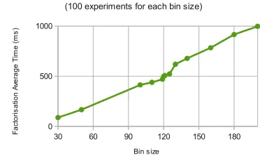
improve performance, in EO-PSI we use hash tables to divide a large set into small subsets and represent each subset as a polynomial. This is a technique that has been used in several regular PSI protocols, e.g. [2], [27]. Intuitively, for a c-element set that is represented by a degree-cpolynomial, the factorization cost isO(c2)
. If we break down the set intohroughly equal-sized subsets, then we will need to factorhpolynomials of degree ch. So, the total cost is reduced toO(c2
h).
In general, hash tables in PSI protocols can be used as follows. First, the public parameters including a random hash functionH, the number of bins in the hash table and the bin’s maximum size are picked. The number of bins in the hash table should be set such that given the maximum set cardinality, with a high probability each bin receives at most a specific number of elements (we will explain shortly how this can be done).
For the parties to compute the set intersection, each of them maps each set element si to the table by computing an address j =H(si), using the hash function whose output is modeled as a uniform random number. Then, it insertssiinto the corresponding binHTj. Because the hash function is deterministic if an element is in the intersection, both parties map it to the same bin. Therefore, a large set of elements can be broken down into a collection of smaller sets (the bins) and a PSI protocol can operate on each bin separately.
As mentioned above, we need to set parameters appropriately to ensure that the number of elements in each bin does not exceed a predefined upper bound. Given the maximum number of elements
c and the bin’s maximum sized, we can determine the number of bins by analyzing hash tables under the balls into bins model which has been extensively studied in the literature [36], [37].
Theorem 1. (Upper Tail in Chernoff Bounds) Let Xi be a
random variable defined asXi= c P
i=1
Yi, whereP r[Yi= 1] =pi, P r[Yi = 0] = 1−pi, and allYiare independent. Let µbe the
expectationE[Xi] = h P
i=1
pi. Then:
P r[Xi> d= (1 +σ)·µ]<
eσ
(1 +σ)(1+σ)
µ
,∀σ >0 (1)
Note that in the balls and bins model the expectation isµ= c
h.
Inequality 1 provides a bound for the probability that bin i is overloaded. Since there arehbins, the probability that at least one of them is overloaded is bounded by theunion bound.
P r[∃i,1≤i≤h:Xi> d]≤ h X
i=1
P r[Xi> d]
≤h· e σ
(1 +σ)(1+σ)
hc (2)
Thus, when the probability and bin’s maximum load are fixed, for anycnumber of elements (as the maximal number of elements that may be inserted into the hash table) we can set the number of bins using inequality 2. In Section 8, some concrete parameters are calculated for our experiments and are shown in Table 3.
3.6 Notation
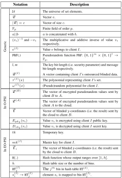
We summarize our notation in Table 1.
TABLE 1 Table of notation.
Notation Description
Generic
U The universe of set elements.
#»
v Vectorv.
|#»v|=c Vector of sizec.
Fp Finite field of orderp.
a||b ais concatenated withb.
(vi)−1and−vi The multiplicative and additive inverse of valuevi respectively.
e(I) Valueebelongs to clientI.
PRF(.) Pseudorandom functionPRF:{0,1}m× {0,1}l→ Fp.
l,m The key bit-length (i.e. security parameter) and message bit-length respectively.
#»
o(I) A vector containing clientI’s outsourced blinded data.
τ(I)(x) The polynomial representing clientI’s set.
ω(I)(x) (Pseudo)random polynomial for clientI.
In
O-PSI
#»
e(B) The vector of encrypted pseudorandom values sent by clientBtoA.
#»
e(A) The vector of encrypted pseudorandom values sent by clientAto the cloud.
#»t Vector of blinded y-coordinates (i.e. the result) sent by
the cloud to clientB.
EpkI(vi) Valueviis encrypted using clientIpublic key.
DskI(vi) Valueviis decrypted using clientIsecret key.
In
EO-PSI
tk Temporary key.
mk(I) Master key for clientI.
#»t
i The vector of blinded y-coordinates (i.e. the result) sent by the cloud to clientB.
H(.) Hash function whose output ranges over[1, h].
h Hash table size or the number of bins.
HT(jI) Thej
thbin in hash table
HT(I).
s(iI)→HTj(I) elementsiis mapped to binHT(jI).
4
O-PSI: OUR
FIRST
PROTOCOL
In this section, we present O-PSI our first protocol for delegated private set intersection on outsourced private datasets.
4.1 An Overview of O-PSI
6
!"#$%&'( !"#$%&') !"#$%&'( !"#$%&') *+, *-, *., #» o ( A )= [ o ( A ) 1 ,. .., o ( A ) n ] #» o ( B )= [ o ( B ) 1 ,. .. ,o ( B ) n ]
ID(B)
#»(e
A )= [ e ( A ) 1 ,. .. ,e ( A ) n ] #»
e(B)= [e(B)
1 , ..., e
(B)
n ] #» t = [ t 1 ,.. ., t n ] ID ( B ) ID ( A ) q1 ,. ..,
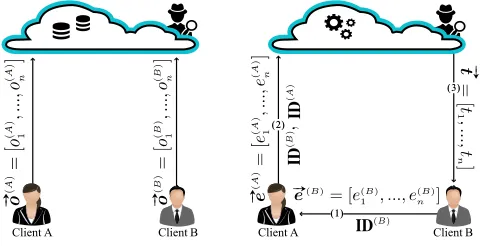
Fig. 1. The left-hand side figure: party interaction at data outsourcing phase in O-PSI; the right-hand side figure: party interaction at the computation delegation phase in O-PSI.
4.2 O-PSI Protocol
Without loss of generality, first, we consider the two client case, where clientA, clientBand a cloud engage in the protocol.
a. Cloud-Side Setup.The cloud picks a public parametercthat is an upper bound of the set cardinality. The cloud constructs a finite fieldFp, where p is a large prime number. It also
constructs a vector#»xcontainingn= 2c+1distinct non-zero
xivalues randomly picked fromFp. It picks a pseudorandom
function PRF: {0,1}m× {0,1}l →
Fp, which takes an
l-bit key and m-bit message, and maps the message to an element in the field pseudorandomly. The cloud publishes the description of the field, the valuen, the vector#»xand the pseudorandom functionPRF.
b. Client-Side Setup and Data Outsourcing. Let client I ∈ {A, B} have a set S(I), where S(I) ⊂ U for some set
universe U and |S(I)| ≤ c. Each client I performs the
following:
1) Generates a Paillier key pair(pkI, skI) (see section 3.2) and publishes the public key. It also chooses a random pri-vate keyk(I)
for the pseudorandom functionPRF. All the keys are generated according to a given security parameter. 2) Constructs a polynomial τ(I)(x) =
|S(I)|
Q
i=1
(x−s(I)
i ) that represents its set S(I). Represent τ(I)(x) as point-value
form, by evaluating it at every elementxiin
#»
x. This yields a vector containing valuesτ(I)(x
i),1≤i≤n. 3) Blinds every value τ(I)(x
i). To do that, it generates a set of pseudorandom values (or blinding factors) z(I)
i =
PRF(k(I), i)
; next, computeso(I)
i as follows:
1≤i≤n:o(I)
i =τ
(I)(x
i)·z
(I)
i
At the end of this step, the set elements are represented as vector #»o(I)= [o(I)
1 , ..., o (I)
n ]. 4) Sends vector #»o(I)to the cloud.
c. Set Intersection: Computation Delegation. This phase starts when client B becomes interested in the intersection of its set and clientA’s set.
1) Client B sends a message to client A. The message contains client B’s ID,ID(B)
, and a vector #»e(B), whose
elements are computed as follows: ∀i,1≤i≤n:e(B)
i =EpkB(z
(B)
i )
wherez(B)
i =PRF(k(B), i)are the values used by clientB to blind its polynomial in step b.3 above.
2) Given clientB’s message, clientAcomputes vector#»e(A)
. ∀i,1≤i≤n:
e(A)
i = (e
(B)
i )(z
(A)
i )
−1
=EpkB(z
(B)
i ·(z
(A)
i )−1) wherez(I)
i =PRF(k(I), i)forI∈ {A, B}are the values from step b.3.
3) ClientAsends#»e(A)
,ID(A)
,ID(B)
, andComputemessage to the cloud.
d. Set Intersection: Cloud-Side Result Computation. 1) After receiving theComputemessage fromA, the cloud
picks two degree c random polynomials ω(A)(x) and
ω(B)(x)(whose coefficients are chosen from
Fp).
2) The cloud fetches the clients outsourced datasets#»o(A)
and
#»
o(B)and then computes vector #»t as below.
∀i,1≤i≤n:
ti= (e
(A)
i )
o(iA)·ω(A)(xi)·E
pkB(ω
(B)(x
i)·o
(B)
i )
=EpkB(z
(B)
i ·(ω
(A)(x
i)·τ
(A)(x
i)+ω
(B)(x
i)·τ
(B)(x
i)))
3) The cloud sends #»t to clientB.
e. Set Intersection: Client-Side Result Retrieval
1) Client B decrypts the elements in #»t and then removes the blinding factors. This yields vector #»g computed as follows:
1≤i≤n:
gi=DskB(ti)·(z
(B)
i )−1=z
(B)
i ·(ω(A)(xi)·τ
(A)(x
i) + ω(B)(x
i)·τ
(B)(x
i))·(z
(B)
i )
−1 = ω(A)(x
i)·τ
(A)(x
i) + ω(B)(x
i)·τ
(B)(x
i)
2) It then interpolates the polynomialφ(x)using the point-value pairs(xi, gi)and considers the valid roots ofφ(x) as the elements in the set intersection (see section 3.3). Remark 1: In step a, the cloud publishes a vector#»xthat has2c+1
elements, because the polynomialφ(x)in step e.2 is of degree2c
and at least2c+ 1points are needed to interpolate it. Note that the elements in#»xare picked at random fromFpso the probability of xibeing a root of a client’s polynomial is negligible.
Remark 2: In step b.3, if the client does not blind the evaluated polynomial and stores the valuesτ(I)(x
i) directly on the cloud, then the cloud could usen pairs of(xi, τ(I)(xi)) to interpolate the client’s polynomial. As a result, the client’s set would be revealed to the cloud. Whereas, when they are blinded the cloud cannot learn anything about the client’s set unless it knows the pseudorandom function key used by the client. The client blinds the values by multiplication; while multiplication cannot blind
τ(I)(x
i) = 0. This is why we require the probability ofxi ∈
#»
x
being a root of a client’s polynomial to be negligible.
Remark 3: The data stored in the cloud are independently blinded by its owner. Also, to compute the set intersection correctly, the blinding factors (z(I)
i in the protocol) must be eliminated at the end of the protocol. In step c.2, clientAandB jointly compute the vector #»e(A)
that allows the cloud to obliviously “switch”A’s blinding factors toB’s. Accordingly, in step d.2, the cloud uses
#»
e(A) to eliminate z(A)
i and replace it with z
(B)
i . The blinding factorsz(B)
i , later on in step e.1, can be eliminated by clientB. What is more, since the values in #»e(A) are encrypted and only
Remark 4: The client’s original blinded dataset remains un-changed in the cloud. In fact, in step d.2, the cloud multiplies a copyof the client’s blinded dataset by the vector ofω(I)(x
i).
Remark 5: The only information that the cloud learns about the clients’ datasets is the upper bound on the datasets cardinality (i.e. value c) that was initially set by itself. Thus, the cloud learns nothing about the exact number of the set elements and the intersection cardinality.
4.3 Multiple Clients O-PSI
With minor modifications, two-client O-PSI can be turned intom -client O-PSI, where m > 2. Below we outline how this can be done. In this case, the client interested in the intersection, client
B, sends the same request (see step c.1 of the protocol) to all other clients,Az, where1 ≤z ≤y andy =m−1. The protocol for each clientAz remains unchanged. For each clientAz, the cloud carries out step d.2 and it computes the result vector#»t as follows: ∀i,1≤i≤n:
ti=EpkB(ω
(B)(x
i)·o
(B)
i )· y Q
z=1
(e(Az)
i )
o(iAz)·ω(Az)(x
i)
=EpkB(z
(B)
i ·(ω
(B)(x
i)·τ
(B)(x
i) + y P
z=1
ω(Az)(x
i)·τ
(Az)(x
i)))
Then, the cloud sends #»t to clientB. Note that in this case, even if clientBcolludes withy−1clients, it could not infer the set elements of the non-colluding client, as the random polynomials
ω(Az)andω(B)are picked by the cloud, and are unknown to the
clients.
5
A MORE
EFFICIENT
PROTOCOL, EO-PSI: OUR
SECOND
PROTOCOL
In this section, we introduce EO-PSI that preserves all O-PSI’s desirable properties and is more efficient. EPSI improves O-PSI from two perspectives. First, unlike O-O-PSI, EO-O-PSI does not use any public key encryption that is computationally expensive. In O-PSI, the public key encryption is mainly used to prevent the cloud from eventually learning any information about the blinding factors (and set elements) during the cloud-side “switching” of the blinding factors, especially when the computation is delegated multiple times. Recall in O-PSI given the vector #»e the cloud can “switch” one client’s blinding factors to another’s. In contrast, in EO-PSI no such “switching” is required. Therefore, no public key encryption is needed. In order to achieve this, we slightly change the way each client blinds its polynomial. In EO-PSI, instead of multiplying valueτ(xi)by a pseudorandom value, the client sums the value and the pseudorandom value. Moreover, the interaction between the clients is changed, in the sense that client Asends a message to both the cloud and clientB when it authorizes the computation.
Second, EO-PSI allows each client to break down its original polynomial into smaller degree polynomials. This allows the result recipient to factorize a set of smaller degree polynomials rather than one of very large degree. As a result, it can find the roots of the polynomials (i.e. the set intersection) faster than in O-PSI. To achieve this, the protocol lets each client insert its elements into the bins of a (fixed-size) hash table.
5.1 An Overview of EO-PSI
The interaction between parties in EO-PSI is depicted in Fig. 2. What follows is a high-level description of the protocol. First,
#»(o
A
)=
[
#»(o
A
)
1
,.
..,
#» o
(
A
)
h
]
#» o
(
B
) =
[
#» o
(
B
)
1
,.
..,
#» o
(
B
)
h
]
!"#$%&'( !"#$%&') !"#$%&'( !"#$%&')
*+, *-, *+,
*.,
mk(B)
tk
#»
q= [q#»1, ...,
# » qh]
#»
t
=
[ #»
t
1
,.
..,
#»
t
h
]
ID
(
B
) ID
(
A
)
q1
,.
..,
q1
,.
..,
ID(B) q1, ...,
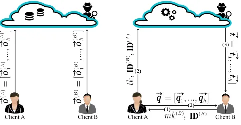
Fig. 2. The left-hand side figure: party interaction at data outsourcing phase in EO-PSI; the right-hand side figure: party interaction at the computation delegation phase in EO-PSI.
each client inserts its set elements into the hash table. Then, it represents the set of elements in each bin of the hash table as a blinded point-value polynomial and sends the polynomials to the cloud. When client B becomes interested in the intersection of its own set and client A’s set, it obtains the client’s permission by sending a message to it. If client Aagrees, it generates a set of vectors and sends them to client B. The vectors help client
B to unblind the cloud’s response. ClientAalso sends a key for a pseudorandom function to the cloud. The key is generated on the fly and is used only in this execution of the protocol. The cloud uses the key and the outsourced datasets to compute a set of blinded polynomials, and sends them to clientB. Given these polynomials and clientA’s message, clientB unblinds them and retrieves the intersection of the sets.
5.2 EO-PSI Protocol
Similarly, here first we consider the two client case, where client
A, clientBand a cloud engage in the protocol.
a. Cloud-Side Setup.The cloud sets the parameters for a hash table. It setscas the upper bound of the set cardinality,das the maximum load that a bin in the hash table can have, and
has the total number of bins in the hash table. Moreover, it chooses a cryptographic hash function,H. Then, the cloud constructs a finite fieldFp, wherepis a large prime number.
It also constructs a vector#»xcontainingn= 2d+ 1distinct non-zero xi values randomly picked from Fp. It picks a
pseudorandom function PRF : {0,1}m× {0,1}l → Fp,
which takes anl-bit key and m-bit message, and maps the message to an element in the field pseudo-randomly. The cloud publishes the hash table parameters, the description of the field, the value n, the vector #»x, the pseudorandom functionPRFalong with the hash functionH.
b. Client-Side Setup and Data Outsourcing.Let client I ∈ {A, B} have a set S(I)
, whereS(I) ⊂ U
and|S(I)| ≤ c
. Each clientIperforms the following:
1) Given the hash table parameters, generates a hash table and inserts its set elements into it, as below.
∀s(I)
i ∈S
(I)
:H(s(I)
i ) =j, thens
(I)
i →HT
(I)
j
where1≤j≤h.
2) Assigns a key (for the pseudorandom function) to each bin in the hash table by picking a master keymk(I), and
8 ∀j,1≤j≤h:k(I)
j =PRF(mk(I), j). 3) For every binHT(I)
j , if it has less thandset elements, pads it with dummy (or random) elements,rj,i, todelements. Then, encodes the bin elements as below.
a) Constructs a polynomial representing the elements in the bin.
τ(I)
j (x) = d Q
i=1
(x−e(I)
i )
wheree(I)
i ∈HT
(I)
j ,e
(I)
i =s
(I)
i ore
(I)
i =rj,i. b) Representsτ(I)
j (x)in point-value form, by evaluating it at every element xi ∈
#»
x. This yields a vector containing valuesτ(I)
j (xi),1≤i≤n. c) Blinds every valueτ(I)
j (xi). To do so first generates a pseudorandom valuez(I)
j,i =PRF(k
(I)
j , i), where key k(I)
j was generated in step b.2. After that, computes o(I)
j,i as follows.
∀j,1≤j≤hand∀i,1≤i≤n:
o(I)
j,i =τ
(I)
j (xi) +z
(I)
j,i
At the end of this step, the elements in bin HTj are represented as the vector #»o(I)
j = [o
(I)
j,1, ..., o (I)
j,n]. 4) Sends#»o(I)= [#»o(I)
1 , ...,
#»
o(I)
h ]to the cloud.
c. Set Intersection: Computation Delegation. This phase starts when client B wants the intersection of its set and clientA’s set.
1) ClientBsendsmk(B)
and its id,ID(B)
, to clientA. 2) Givenmk(B)
andmk(A)
clientAregeneratesk(I)
j (see step b.2) where1≤j≤hand∀I, I ∈ {A, B}.
3) ClientAassigns three fresh keys to each binHTj. To do that, first, it picks a temporary keytkand then carries out the following.
a) It uses the key, tk, to generate three pseudorandom valueskt.
∀t,1≤t≤3:kt=PRF(tk, t). b) It uses eachktto computehpseudorandom values.
∀j,1≤j≤h:k1,j=PRF(k1, j),k2,j=PRF(k2, j),
k3,j=PRF(k3, j).
4) For each binHTj clientAuses keyk1,j to generate a set of pseudorandom valuesaj,i.
∀i,1≤i≤n:aj,i=PRF(k1,j, i).
Also, it uses keyk2,j andk3,j to generate two degree d pseudorandom polynomialsω(A)
j (x)andω
(B)
j (x)for that bin.
5) For each binHTj clientA regenerates the pseudorandom valuesz(A)
j,i =PRF(k
(A)
j , i)andz
(B)
j,i =PRF(k
(B)
j , i)using the keys it derived in step c.2. Then, it computes vectorq#»j as follows.∀i,1≤i≤n:
qj,i=z
(A)
j,i ·ω
(A)
j (xi) +z
(B)
j,i ·ω
(B)
j (xi) +aj,i
Vectorsq#»j allow clientB to remove the blinding factors from the cloud’s response without learning the pseudoran-dom polynomials.
6) Client A sends #»q = [#»
q1, ...,
# »
qh]to clientB. Also, client Asends the keytk (generated in step c.3),ID(A)
,ID(B)
,
andComputemessage to the cloud.
d. Set Intersection: Cloud-Side Result Computation. 1) Given the keytk, the cloud derives the three keysk1,j,k2,j
andk3,jfor each binHTj, where1≤j≤h(see steps c.3a and c.3b)
2) Using the keys generated in the previous step, the cloud regenerates the set of pseudorandom valuesaj,i(∀i,1 ≤ i ≤ n) and the two pseudorandom polynomialsω(A)
j (x) andω(B)
j (x)for each binHTj, where1≤j≤h(see step c.4).
3) The cloud computes the result as follows. First, it fetches the clients’ outsourced datasets#»o(A)
j and
#»
o(B)
j in each bin HTj. Next, it computes the result vectort#»j for that bin as below.
∀j,1≤j≤hand∀i,1≤i≤n:
tj,i=o
(A)
j,i ·ω
(A)
j (xi) +o
(B)
j,i ·ω
(B)
j (xi) +aj,i
4) The cloud sends #»t = [t#»1, ...,
#»
th]to clientB. e. Set Intersection: Client-Side Result Retrieval
1) Client B removes the blinding factors from each vector
#»
tj (∀j,1 ≤ j ≤ h) using the corresponding vector
#»
qj (provided by clientAin step c.6). The result is the vector
#»
gjcomputed as follows.
∀j,1≤j≤hand∀i,1≤i≤n:
gj,i=tj,i−qj,i=ω
(A)
j (xi)·τ
(A)
j (xi)+ω
(B)
j (xi)·τ
(B)
j (xi)
2) Given each vectorg#»jand
#»
xit interpolates the polynomial
φj(x)(∀j,1≤j≤h).
3) It extracts the roots of each polynomial. It considers the union of the valid roots as the intersection of the sets. Remark 1: ClientI can always update (or replace) the blinding factors of its outsourced dataset in the cloud without leaking any information to it. To do so, it picks a fresh master keymk0(I), and
deriveshkeysk0(I)
j from the master key: ∀j,1≤j≤h:k0(I)
j =PRF(mk0(I), j) Next, it uses each keyk0(I)
j to generatenpseudorandom values z0(I)
j,i for each bin:
∀j,1≤j≤h,∀i,1≤i≤n:z0(I)
j,i =PRF(k
0(I)
j , i)
Also, it uses its old master key to regenerate the blinding factorsz(I)
j,i used to blind the outsourced dataset. Then, for every bin it computes the following values:
∀j,1≤j≤h,∀i,1≤i≤n:u(I)
j,i =−z
(I)
j,i +z
0(I)
j,i
It sends allu(I)
j,i to the cloud and asks it to sum them with the corresponding blinded values o(I)
j,i = τ
(I)
j (xi) +zj,i(I). After the cloud follows its instruction it would get the following blinded values:
∀j,1≤j≤h,∀i,1≤i≤n:
o0(I)
j,i =o
(I)
j,i +u
(I)
j,i =τ
(I)
j (xi) +z
0(I)
j,i
Now, the client can discard its old master key and only needs to keepmk0(I)
locally.
the computation. To avoid this, the server sets the parameters including the number of bins, the maximum load of each bin and the maximum set cardinality in such a way that the probability of any bin exceeding its capacity is negligible. The parameters can be derived by the cloud using inequality 2 (provided in section 3.5 with example values shown in Table 3).
Remark 3: In EO-PSI, the client needs to find the roots of h
polynomials of degree 2d, where d is a fixed value picked by the cloud and it is much smaller than the maximum number of elements, c. In contrast, in O-PSI the client receives only one polynomial of degree2c. Clearly, finding roots ofhpolynomials of small degree 2d is much faster than finding the roots of one polynomial of very large degree 2c and our performance evaluation in section 8 also supports this (see Fig. 4).
Remark 4: In both EO-PSI and O-PSI, the cloud-side setup is performed only once, when the cloud comes online. Afterward, it does not need to do any computation in this step. Furthermore, none of our protocols requires the participation of a trusted third party.
Remark 5: Bloom filters can be used in PSI Protocols to improve their efficiency [25]. A Bloom filter encodes a set and allows membership queries. In traditional PSI, the parties have a local copy of their own sets, so they can query the filters using the sets to get the intersection. In delegated PSI, clients outsource their data and do not keep a local copy. A delegated PSI protocol based on Bloom filters would require clients to enumerate the universe of the set elements in order to get the intersection. For this reason, we do not use Bloom filters in our protocol.
Remark 6: Public key cryptography preserves certain algebraic properties, therefore protocols based on it can be simpler and more intuitive than those based on symmetric key cryptography. For this reason, we first design the O-PSI protocol to show feasibility, then the EO-PSI protocol to improve efficiency.
5.3 Multiple Clients EO-PSI
With minor adjustments, the protocol can supportm >2number of clients. Here, we denote the result recipient by clientBand the other clients byAz,∀z,1≤z≤yandy=m−1.
Similar to the two clients case, here each clientAz sends to the cloud a temporary key tk(Az) that lets the cloud generate
for each bin HTj a set of pseudorandom values a(Az)
j,i and two pseudorandom polynomialsω(Az)
j (x)andω
(Bz)
j (x). However, as it is shown below, the cloud-side computation in step d.3 is slightly changed.∀j,1≤j≤hand∀i,1≤i≤n:
tj,i=o
(B)
j,i ·ω
(B)
j (xi) + y P
z=1
a(Az)
j,i + y P
z=1
o(Az)
j,i ·ω
(Az)
j (xi)
whereω(B)
j (x) = y P
z=1
ω(Bz)
j (x)
Note, in the above step the cloud first adds all the polynomials
ω(Bz)
j (x)together, then it evaluates the result polynomial at every element in #»x, and next multiplies the result by clientB’s blinded values for that bin (i.e. binHTj).
Consequently, clientBin step e.1 removes the blinding factors from vectort#»j as follows:
gj,i=tj,i− y P
z=1
q(Az)
j,i
=ω(B)
j (xi)·τ
(B)
j (xi) + y P
z=1
ω(Az)
j (xi)·τ
(Az)
j (xi)
In multiple clients EO-PSI, even if clientBcolludes withy−1
clients, it cannot learn any information about the non-colluding
client’s set elements. The reason is that, as it is shown in [21], the polynomialω(B)
j (x)is always a uniformly random polynomial even if only one of the polynomialsω(Bz)
j (x)is uniformly random and unknown to clientB.
Remark 1: In multiple client EO-PSI, the communication and computation complexities for those clients who authorize the com-putation (i.e. clientsAz) are independent of the number of clients participating in the protocol. In other words, the computation and communication complexities for clientA in the two client case are similar to clientAj’s in the multiple clients case. Note that the same holds for multiple client O-PSI.
Remark 2: In multiple client EO-PSI, each client Aj indepen-dently authorizes the computation, without the need to interact with the other authorizing clients. The same is true for multiple client O-PSI.
6
PROOF OF
SECURITY
Now we present the proof of EO-PSI security in the semi-honest model. The security proof of PSI can be found in [1]. O-PSI and EO-O-PSI are both proved using the ideal-real paradigm. However, there are some differences between the proofs: (1) the security relies on different assumptions, in O-PSI it relies on the assumption of the existence of a semantically secure additive homomorphic encryption scheme, while in EO-PSI it relies on the assumption of the existence of a secure pseudorandom function; (2) in O-PSI the clients’ blinded input sets are represented as a single polynomial, while in EO-PSI, the sets are split into bins and each bin is represented as a polynomial.
Theorem 2. If PRF is a pseudorandom function, then EO-PSI
protocol is secure in the presence of a semi-honest adversary.
Proof. We will prove the theorem by considering, in turn, the case where each of the parties has been corrupted. In each case, we invoke a simulator with the corresponding party’s input and output. Our focus is in the case where partyAwants to engage in the computation of the intersection. If partyAdoes not want to proceed with the protocol, the views can be simulated in the same way up to the point where the execution stops.
Case 1: Corrupted Cloud. In this case, we show that we can construct a simulatorSimC that can produce a computationally indistinguishable view. In the real execution, the cloud’s view,
ViewπC(Λ, S(A), S(B))
, is as follows: {Λ, rC,
#»
o(A)
,#»o(B)
, tk,ID(A)
,ID(B)
,Compute,Λ}
In the above view,rCis the outcome of internal random coins of the cloud, #»o(A),#»o(B) are the hash tables each containing the
blinded set representations ofA’s andB’s sets, andtkis anl-bit random key used in the protocol to generate the pseudorandom polynomials and the blinding factors to mask the result generated by the cloud.
To simulate this view,SimC does the following: it creates an empty view and appends to itΛand uniformly at random chosen coinsr0C. It uses the public parameters and the hash function to construct two hash tables HT0(A) and
HT0(B). Then, it fills each
bin of the hash tables with n uniformly random values picked from the same field Fp; so each bin HT0j(I) (∀I, I ∈ {A, B}) contains the vector #»o0(I)
j of n random values. It also chooses a key tk0. Afterward, it appends #»
o0(A) = [#»o0(A) 1 , ...,
#»
o0(A)
h ],
#»
o0(B) = [#»o0(B) 1 , ...,
#»
o0(B)
10 simulator appendsID(A),ID(B),Compute
andΛ, to the view and outputs the view.
We argue that the simulated view is computationally indistin-guishable from the real view. In both views, the input parts are identical (i.e. both are Λ), the random coins are both uniformly random, and so they are indistinguishable. In the real model, the elements in #»o(I) ( ∀I, I ∈ {A, B}) are blinded with the
outputs of a pseudorandom function. Also, the elements in #»o0(I)
are random elements of the field. As the blinded values and random value are indistinguishable, the vectors #»o(I)
i and
#»
o0(I)
i are indistinguishable; thus, the vectors #»o(I)
and #»o0(I)
are also indistinguishable. As the keystkandtk0are picked uniformly at
random, they are computationally indistinguishable as well. What is more,ID(A),ID(B)andComputein both models are identical.
Moreover, the output parts in both views are identical (i.e. both areΛ). So, we conclude that the views are indistinguishable. Case 2: Corrupted clientA.In the real execution, theA’s view is as follows:
ViewπA(Λ, S
(A)
, S(B)
) ={S(A)
, rA, mk
(B)
,ID(B)
,Λ}
The simulatorSimAdoes the following: it creates an empty view. It receives the party’s inputS(A)
and appends it to the view. Then, it inserts uniformly at random chosen coinsr0
Ato it. Next, it picks anl-bit keymk0(B)uniformly at random and appends it to
the view. After that, it insertsID(B)
andΛinto the view. In both models S(A)
is identical. Moreover, both rA andr0A are picked uniformly at random so they are indistinguishable. Since both keysmk(B)andmk0(B)are chosen uniformly at random they are
computationally indistinguishable, too. Moreover,ID(B)
andΛare identical in both models. So, the two views are indistinguishable. Case 3: Corrupted client B.In the real execution, client B’s view is as follows:
ViewπB(Λ, S
(A)
, S(B)
) ={S(B)
, rB,
#»
g,#»q, f∩(S
(A)
, S(B)
)}
The simulator SimB receives the party’s input (S
(B)) and
output (f∩(S
(A), S(B))
), and does the following: 1) Creates an empty view, then appendsS(B)
and uniformly at random chosen coinsr0
Bto it.
2) Picks two setsS0(A) and S0(B) such thatS0(A)∩S0(B) =
f∩(S
(A), S(B))
and|S0(A)|,|S0(B)| ≤c
. 3) Constructs the hash tablesHT0(A)and
HT0(B)using the public
parameters. Next, maps the elements inS0(A) andS0(B) to
the bins ofHT0(A)
andHT0(B)
, respectively.∀I, I ∈ {A, B} and∀s0(I)
i ∈S0(I):H(s
0(I)
i ) =j, thens
0(I)
i →HT0j(I), where
1≤j≤h.
4) For each bin constructs a polynomial representing its ele-ments. If a bin contains less thatdelements first it is padded with dummy values,r0(I)
j,i , todelements.∀I, I∈ {A, B}and ∀j,1≤j≤h:τ0(I)
j (x) = d Q
i=1
(x−e(I)
i ), wheree
(I)
i ∈HT0j(I), e(I)
i =s
0(I)
i ore
(I)
i =r
0(I)
j,i .
5) Assigns a random polynomialω0(I)
j of degreedto each bin HT0(I)
j (∀j,1 ≤ j ≤ h) of the hash tableHT
0(I) (∀I, I ∈
{A, B}).
6) Constructs the vectors #»g0
j whose elements are computed as follows.∀j,1≤j≤hand∀i,1≤i≤n:
g0
j,i=τ
0(A)
j (xi)·ω
0(A)
j (xi) +τ
0(B)
j (xi)·ω
0(B)
j (xi)
where τ0(I)
j (x) is the polynomial representing the set of elements contained in binHT(I)
j .
7) Picks a keymk0and deriveshkeys,k0
j, from it as below. ∀j,1≤j≤h:k0
j =PRF(mk
0, j)
8) Uses each keyk0
j to generate
#»
q0
j whose elements are com-puted as follows.
∀j,1≤j≤hand∀i,1≤i≤n:q0
j,i=PRF(k
0
j, i)
9) Adds#»g0= [#»
g0
1, ...,
#»
g0
h]and
#»
q0= [#»
q0
1, ...,
#»
q0
h]to the view. 10) Finally, inserts,f∩(S(A), S(B))to the view.
Now we show that the two views are computationally indis-tinguishable. In both modelsS(B)is identical. As r
B andr0B are chosen uniformly at random, they are indistinguishable.
In the real model, the elements in #»qj are blinded by the outputs of a pseudorandom function. So the blinded elements are uniformly random values. On the other hand, in the ideal model the elements in #»q0
j are the outputs of a pseudorandom function. Hence, the elements in both vectors#»q and#»q0are computationally indistinguishable.
Furthermore, in the real model, given each unblinded vec-tor #»gj, the adversary interpolates a polynomial of the form φ(x)j = ω
(A)
j (x) · τ
(A)
j (x) + ω
(B)
j (x) · τ
(B)
j (x) = µj · gcd(τ(A)
j (x), τ
(B)
j (x)), where µj is a uniformly random poly-nomial andgcd(τ(A)
j (x), τ
(B)
j (x)) represents the intersection of the set elements in the corresponding bin. Similarly, in the ideal model, each polynomial φ0
j(x)interpolated from vector
#»
g0
j has the formφ0
j(x) = ω
0(A)
j (x)·τ
0(A)
j (x) +ω
0(B)
j (x)·τ
0(B)
j (x) = µ0
j ·gcd(τ
0(A)
j (x), τ
0(B)
j (x)), where µ0j is a uniformly random polynomial. As mentioned in section 3.3, it has been shown in [21] that the polynomials φj(x)and φ0j(x)(for each bin) only contain information about the intersections of the corresponding sets and have the same distribution in both models. Finally, in both views the output part (i.e.f∩(S(A), S(B))) is identical. Hence, the
two views are computationally indistinguishable.
Combining the above, we conclude the protocol is secure and complete our proof.
Thus, both the O-PSI and EO-PSI protocols are secure in the semi-honest model and we have proven their security using the real-ideal paradigm. In the proof, we used standard assumptions and did not rely on non-standard ones (e.g. random oracle model).
7
COMPARISON
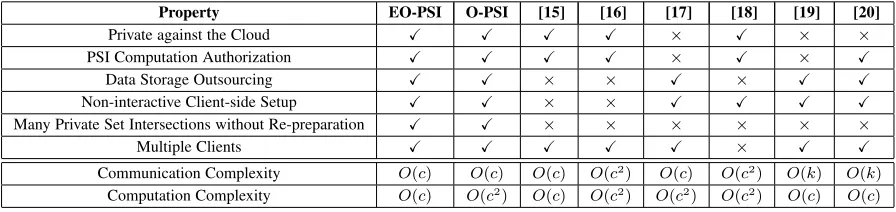
We first evaluate EO-PSI and O-PSI by comparing their properties to those provided by other protocols that delegate PSI compu-tation to a cloud. We also compare these protocols in terms of communication and computation complexity. Table 2 summarizes the results.
Properties.When PSI computation is delegated to a server who is not fully trusted, protecting the privacy of the computation input and output from the server is crucial. However, as discussed in section 2 the protocols in [17], [19], [20] do not fully preserve data privacy and leak some information to the cloud server. Protocols like the size-hiding variation of [15], those in [16], [18], O-PSI and EO-PSI offer this protection.
![TABLE 5Running time (in seconds) of the protocol in [18]](https://thumb-us.123doks.com/thumbv2/123dok_us/7980911.1323757/15.612.311.561.110.183/table-running-time-seconds-protocol.webp)
