A Robust Diffusion Estimation Algorithm with
Self-adjusting Step-size in WSNs
Feng Chen1,†,‡, Qing Ye2,‡, Xiaodan Shao2,‡and Shukai Duan2,*
1 Department of College of Electronic and Information Engineering, School of Mathematics and Statistics, Southwest University, and Key Laboratory of Nonlinear Circuits and Intelligent Information Processing, Chongqing 400715, China. e-mail: ([email protected])
2 Department of College of Electronic and Information Engineering, Southwest University, Chongqing 400715, China. e-mail: ([email protected], [email protected])
* Correspondence: [email protected]; Tel: +023-68251252
† Current address: No.2, Tiansheng Road, Beibei District, Chongqing City, China ‡ These authors contributed equally to this work.
Abstract:In wireless sensor networks (WSNs), each sensor node can estimate the global parameter from the local data in distributed manner. This paper proposed a robust diffusion estimation algorithm based on minimum error entropy criterion with self-adjusting step-size, which are referred to as diffusion MEE-SAS (DMEE-SAS) algorithm. The DMEE-SAS algorithm has fast speed of convergence and is robust against non-Gaussian noise in the measurements. The detailed performance analysis of the DMEE-SAS algorithm is performed. By combining the DMEE-SAS with diffusion minimum error entropy (DMEE) algorithms, an Improving DMEE-SAS algorithm is proposed, in non-stationary environment where tracking is very important. The Improving DMEE-SAS algorithm can avoid insensitivity of the DMEE-SAS algorithm due to the small effective step-size near the optimal estimator, and obtain a fast convergence speed. Numerical simulations are given to verify the effectiveness and advantages of these proposed algorithms.
Keywords:robust diffusion estimation; self-adjusting step-size; non-Gaussian noise; wireless sensor networks
1. Introduction
Distributed estimation has become very popular for parameter estimation in wireless sensor networks. The objective is to enable the nodes to estimate a vector of parameters of interest from the observed data. Distributed estimation schemes over adaptive networks can be mainly classified into incremental strategies [15–17], consensus strategies [18,25], and diffusion strategies [3,4,7,12,19,27]. In the incremental strategies, data is processed in a cyclic fashion through the network. The consensus strategies rely on the fusion of intermediate estimates of multiple neighboring nodes. In the Diffusion strategies, information is processed at all nodes while the nodes communicate with all their neighbors to share their intermediate estimates. The diffusion strategies are particularly attractive because they are robust, flexible and fully-distributed, such as the diffusion least mean squares (DLMS) algorithm [7]. In this paper, we focus on the diffusion estimation strategies.
suffers from conflicting requirements between convergence rate and the steady-state mean square error. A large step-size leads to a fast convergence rate, but a large mean-square error at the steady state.
In this paper, we incorporate the minimum error entropy criterion with self-adjusting step-size (MEE-SAS) [8] into the cost function in diffusion distributed estimation. Then we figure out the diffusion-strategy solutions, which are referred to as the diffusion MEE-SAS (DMEE-SAS) algorithm. Numerical simulation results show that DMEE-SAS algorithm outperforms DLMS, DLMP and DMEE algorithms when the noise is modeled to be non-Gaussian noise. We also design an Improving DMEE-SAS algorithm by using a switching scheme between DMEE-SAS and DMEE algorithms for non-stationary environment, which tracks the changing estimator very effectively. The Improving DMEE-SAS algorithm can avoid the small effective step-size of DMEE-SAS algorithm when it close to the optimal estimator.
We organize the paper as follows. In section 2, we briefly revisit the MEE-SAS algorithm. In section 3, firstly, we propose the DMEE-SAS algorithm and analyze the mean and mean square performance for DMEE-SAS algorithm. Then we propose the Improving DMEE-SAS algorithm for non-stationary scenario. Simulation results are shown in section 4. Finally, we draw conclusions in section 5.
2. The Review of MEE-SAS Algorithm
A convenient evaluation of the integral operator in the formulation of quadratic Renyi’s entropy using Gaussian kernel is obtained as follows:
H(e) =−log( 1
N2
N
∑
i=1
N
∑
j=1
Gσ√2(ej−ei))
=−log(V(e)).
(1)
Wheree= [e1,e2,· · ·,eN]and
Gσ√2(ej−ei)= 1
σ
√ 2π
exp(− 1
2σ2(ej−ei) 2).
V(e) = 1
N2
N
∑
i=1
N
∑
j=1 Gσ√
2(ej−ei)≤V(0) =
1
σ
√ 2π
.
The information potentialV(e)is defined as the argument of the log. The maximum valueV(0) of the information potential will be achieved whene1=e2=· · ·=eN. The above results are obtained
in the case of batch mode, where theNdata points are fixed. For online training methods, we estimate the parameter using the stochastic information potential given below
V(e)≈ 1
L
i
∑
j=i−L+1 Gσ√
2(ei−ej). (2)
WhereLis the latestLsamples ofe.
To minimize the entropy is equivalent to maximize the information potential since the log is a monotonic function. To maximize the information potential is equivalent to minimize the following cost function. Therefore, the cost function of MEE-SAS algorithm is
The MEE-SAS method has shown its ability to achieve faster speed than minimum error entropy (MEE) method and is robust to outliers. Based on these properties, we develop the diffusion MEE-SAS algorithms in the next section.
3. Proposed Algorithm
In this section, first, the diffusion MEE-SAS (DMEE-SAS) algorithm is proposed. Second,
the detailed convergence and steady-state analyses of this algorithm are performed. Finally, an Improving scheme for diffusion DMEE-SAS algorithm is carried out to use in non-stationary scenario.
3.1. Diffusion MEE-SAS Algorithm
Consider a connected wireless sensor networks withK nodes. k ∈ {1, 2, . . . ,N} is the node index andiis the time index. To proceed with the analysis, we assume a liner measurement model as follows:
dk,i=uTk,iw0+vk,i. (4)
Wherew0is aM×1 deterministic but unknown vector,d
k,iis a scalar measurement of some random
process,uk,iis theM×1 regression vector at time with zero mean and covarianceσu2,vk,iis the random
noise signal at timeiwith zero mean and varianceσv2. For each node, we have
V(ek,i) =
1
L
i
∑
j=i−L+1 Gσ√
2(ek,i−ek,j)≤V(0) =
1
σ
√ 2π
. (5)
Whereek,i = dk,i−uTk,iw. The maximum value V(0)will be achieved whenek,i = ek,j, j = i−L+
1,i−L+2,· · ·,i.
We seek an estimate of w0 by minimizing a linear combination of local information. The
individual local cost function for each nodekis calculated as
Jk(w) =
∑
l∈Nkcl,kE[V(0)−V(el,i)]2. (6)
Nk denotes the one-hop neighbor set of node k, and {clk} are some non-negative cooperative
coefficients satisfyingclk = 0 if l ∈/ Nk, 1TC¯ = 1T and ¯C1 = 1. Here, ¯Cis a N×N matrix with
individual entries{clk}and 1 is a N×1 all-unity vector. The gradient of the individual local cost
function is given by
∇Jk(w) =
∑
l∈NkclkE[( 2
σ2L)(V(0)−V(ek,i))
i
∑
j=i−L+1
Gσ√2(ek,i−ek,j)(ek,i−ek,j)(uk,j−uk,i)]. (7)
We remove the expectation to generate stochastic gradient updates, then the (7) can be rewritten as
∇Jˆk(w) =
∑
l∈Nk clk(
2
σ2L)(V(0)−V(ek,i))
i
∑
j=i−L+1 Gσ√
2(ek,i−ek,j)(ek,i−ek,j)(uk,j−uk,i). (8)
A gradient based algorithm for estimatingw0at each nodekcan thus be derived as wk,i =wk,i−1−µk∇Jˆk(w)
=wk,i−1−µk
2
σ2Ll∈
∑
N kclk[V(0)−V(ek,i)] i
∑
j=i−L+1 Gσ√
2(ek,i−ek,j)(ek,i−ek,j)(uk,j−uk,i).
Whereµkis a positive step size. Using the general framework for diffusion-based distributed adaptive
optimization [12], an adapt-then-combine (ATC) strategy for diffusion MEE-SAS algorithm can be formulated as
ϕk,i =wk,i−1−µkσ22L[V(0)−V(ek,i)] i
∑
j=i−L+1 Gσ√
2(ek,i−ek,j)(ek,i−ek,j)(uk,j−uk,i),
wk,i = ∑ l∈Nk
clkϕl,i.
(10)
According to (10), the DMEE-SAS algorithm can be seen as a diffusion estimation algorithm with variable step sizeµk(i). Where
µk(i) =2µk[V(0)−V(ek,i)]. (11)
The DMEE-SAS algorithm is described formally in Algorithm 1.
Algorithm 1: DMEE-SAS Algorithm
Initialize:wk,i=0
fori=1 :T for each nodek:
Adaptation
µk(i) =2µk[V(0)−V(ek,i)]
ϕk,i=wk,i−1−µk(i)σ12L i
∑
j=i−L+1
G σ
√
2(ek,i−ek,j)(ek,i−ek,j)(uk,j−uk,i)
Combination wk,i= ∑
l∈Nk clkϕl,i
end for
In the adaption step of DMEE-SAS algorithm,V(0)−V(ek,i)is close toV(0)when the algorithm
starts, and it is close to 0 when the algorithm begins to converge. V(0)−V(ek,i) is always
a non-negative scalar quantity, which can accelerate the rate of convergence and achieve small steady-state estimation errors. The fast convergence rate and the small steady-state estimation errors of DMEE-SAS algorithm can be established against non-Gaussian noise in the measurements.
3.2. Performance Analysis
In this section, we analyze the mean and mean-square performance of the DMEE-SAS algorithm. For tractability of the analysis, here we fous on the case of batch mode. To briefly present the convergence property of the proposed algorithm in terms of global quantities, the following notations are introduced: Mτ = diag{µ1(τ)IM, . . . ,µK(τ)IM}, Wτ = col{w1,τ,· · ·wK,τ}, w(0) =
col{w0,· · ·,w0}, ˜Wτ = col{w˜1,τ· · ·w˜K,τ},S = col{s1(w0),· · ·,sK(w0)},C = C¯T⊗IM. τ denotes the iteration index.
In order to make the analysis tractable, the followings are assumed:
Assumption 1: The regressor uk,i is independent identically distributed (i.i.d) in time and
spatially independent, andE[uk,i] =0,Rk=E[uTk,iuk,i].
Assumption 2: The input noisevk,i is super-Gaussian noise. In addition,vk,i and the regressor
uk,iis independent from each other. we haveE[vk,i] =0 andE[v2k,i] =ξ2k.
Assumption 3: The step-sizes, µk(i),∀k, are small enough such that their squared values are
3.2.1. Mean performance
When we consider the variable step sizeµk(i)of DMEE-SAS algorithm as a new step size factor,
we can also seek the optimal estimatorw0by minimizing the following individual local cost function Gk(w) =
∑
l∈Nk
clkE(V(0)−V(el,i)). (12)
Where
V(el,i) = 1
N2
N
∑
i=1
N
∑
j=1
Gσ√2(el,i−el,j)
We obtain the first gradient ofE(V(0)−V(ek,i))as follows
gk(w) =E( 1
σ2N2Gσ
√
2(ek,i−ek,j)(ek,i−ek,j)(uk,j−uk,i)]. (13)
The instantaneous implementation for (13) is as follows
ˆ
gk(w) = 1
σ2N2
N
∑
i=1
N
∑
j=1
Gσ√2(ek,i−ek,j)(ek,i−ek,j)(uk,j−uk,i). (14)
We consider the gradient error caused by approximating the expectations with their instantaneous values [9]. The gradient error at iterationτand each nodekis defined as follows:
sk(wk,τ−1) =gˆk(wk,τ−1)−gk(wk,τ−1). (15) Using (10), the update equation of the intermediate estimate can be rewritten as
ϕk,τ=wk,τ−1−µk(gk(wk,τ−1) +sk(wk,τ−1)). (16)
According to [29], ((ek,i−ek,j)/σ=0 whenw=w0. And the Hessian matrix functionHk(w0)ofJk(w)
is calculated as
Hk(w0) =
∂gk(w)
∂w |w0
= ∂
∂w
1
σ2E[Gσ
√
2(ek,i−ek,j)(ek,i−ek,j)(uk,j−uk,i)]
= 1
σ2E[Gσ
√
2(ek,i−ek,j)(uk,j−uk,i)T(uk,j−uk,i)−
1
σ2Gσ
√
2(ek,i−ek,j)(ek,i−ek,j)2(uk,j−uk,i)T(uk,j−uk,i)]
= 1
σ2E[u
T
k,iuk,i+ukT,juk,j]−
1
σ4E[v 2 k,i +v
2 k,j]E[u
T
k,iuk,i+uTk,juk,j]
= 2Rk
σ2 −
4ξ2kRk
σ4 .
(17)
Based on the Theorem 1.2.1 of [10], we obtain
gk(wk,τ−1) =gk(w
0)−(Z 1 0 Hk
(w0−xw˜k,τ−1)dx)w˜k,τ−1 =−(
Z 1
0 Hk(w 0−xw˜
k,τ−1)dx)w˜k,τ−1.
Where ˜wk,τ−1 = w0−wk,τ−1is the weight error vector for nodek. We assume that the estimate of
each node converges to the vicinity of the unknown vectorw0. Therefore ˜wk,τ−1is small enough such that it is negligible, yielding
gk(wk,τ−1) ≈ −(
Z 1
0 Hk
(w0)dx)w˜k,τ−1 =−Hk(w0)w˜k,τ−1.
(19)
We can also obtain the approximation of the gradient error at the vicinity ofw0, which is given by
sk(wk,ø−1) ≈sk(w0)
=gˆk(w0)−gk(w0)
= 1
σ2
N
∑
i=1
N
∑
j=1 Gσ√
2(vk,i−vk,j)(vk,i−vk,j)(uk,j−uk,i).
(20)
Substituting (19) and (20) into (16), an approximation of intermediate estimate can be obtained at the vicinity of
ϕk,τ =wk,τ−1+µk(τ)(Hk(w0)w˜k,τ−1−sk(w0)). (21)
By substituting (21) into the second equation of (10), we get the estimate of unknown parameter as follows
wk,τ =
∑
l∈Nk
clk[wl,τ−1+µk(i)(Hk(w
0)w˜
l,τ−1−sl(w
0))]. (22)
Using global quantities defined above gives the update equation for the network estimate vector as
Wτ=C(Wτ−1+MτHW˜τ−1−MτS). (23)
Where H collects the Hessian matrix across the network into the global vector H =
diag(H1(w0),· · ·,HN(w0)). Noting thatCw(0)=w(0), subtraction of both sides of (23) fromw0gives
˜
Wτ =C(IMN−MτH)W˜τ−1+CMτS. (24) In view of assumptions A1 and A2, ˜Wτ, H and C are independent of each other. Hence taking expectation of both sides of (24) leads to
E[W˜τ] =E[C](IMN−E[Mτ]H)E[W˜τ−1] +CMτE[S]. (25) We can easily find thatE[S] =col{E[s1(w0),· · ·,sN(w0)]}=0, the equation (25) has therefore been
reduced to this form
E[W˜τ] =E[C](IMN−E[Mτ]H)E[W˜τ−1]. (26) From (26), we observe that in order to be stable for the Algorithm 1 in the mean sense, the matrix
E[C](IMN−E[Mτ]H)should be stable. All the entries ofE(C)are non-negative and all the rows of it add up to unity. Therefore, to ensure the stability in the mean, it should hold that
|λmax{IMN−E[Mτ]H}|<1. (27)
We use the notionλmax(A)to denote the maximum eigenvalue of a Hermitian matrix A. The
algorithm will therefore be stable in the mean if
∞
∏
τ=0Thus, we note that a sufficient condition for unbiasedness is
0<E[µk(τ)]< 2 λmax{Hk(w0)}
⇔0<µk <
1
λmax{Hk(w0)}E[V(0)−V(ek,τ)]
. (28)
3.2.2. Mean-square Performance
In order to make the presentation clearer, we shall introduce the following notation
Γ= (IMN−MτH)CTΣC(IMN−MτH).
Performing weighted energy balance on both sides of (24), and taking expectations gives
E[ W˜τ
2
Σ] =E[
W˜τ−1
2
Γ] +E[STMτCTΣCMτS]. (29) Where Σ is an arbitrary symmetric nonnegative-definite matrix, and the notion kak2Σ = aTΣa
represents a weighted vector norm for any HermitianΣ>0. By defining
r=vec{E[Γ]},`=vec{Σ}.
Where the vec(.) notation stacks the columns of its matrix argument on top of each other. We can modify (29) to
E[W˜τ 2 `] =E[
W˜τ−1
2
r] +E[S TM
τCTΣCMτS]. (30)
Using the following relationship of the vectorization operator and the Kronecker product [28]:
vec(ABC) = (CT⊗A)vec{B}. We can obtain that
r=φ`. (31)
Where
φ=E[(IMN−E[Mτ]H)⊗(IMN−E[Mτ]H)]β. (32)
β=E[CT⊗CT].
Considering Assumption 3, we can approximate (32) as
φ ≈(IM2N2−IMN⊗E[Mτ]H−E[Mτ]H⊗IMN)β
= (IMN−E[Mτ]H)⊗(IMN−E[Mτ]H)β.
(33)
Using the following relationship of the vectorization operator and the matrix trace [28]:
Tr{ATB}=vecT(B)vec(A). We find that
E[STMτCTΣCMτS] =vecTQβθ. (34) Where
Q=E[MτSS
TM
τ].
Substituting (31) and (34) into (30), we can then reformulate recursion as follows
E[ W˜τ
2 `] =E[
W˜τ−1
2
φθ] +vec
TQ
It is known that (35) is stable and convergent if the matrixφis stable [11]. Form the equation
βT1M2N2 =E[(C⊗IM)1MN⊗(C⊗IM)1MN] =1M2N2.
We know that all the entries ofβin (34) are non-negative and all its columns sum up to unity. Using
the propertyλ(A⊗A) =λ2(A), the stability ofφhas the same conditions as the stability ofIMN− E[Mτ]H. Therefore, we choose the step size in accordance with (28) which can keep the DMEE-SAS stable in the mean-square sense.
3.3. An Improving Scheme for DMEE-SAS Algorithm
The too small effective step size near the optimal estimator will hinder the tracking ability of DMEE-SAS algorithm in non-stationary environment. In non-stationary environment, the optimal estimator has small changes. A random-walk model is commonly used in the literature to describe the non-stationarity of the weight vector [11].
Therefore, we try to combine the DMEE-SAS algorithm with DMEE algorithm [6] in
non-stationary environment where tracking is important. DMEE-SAS algorithm should be used due to the faster convergence when the algorithm start, and DMEE algorithm should be used when algorithm begins to converge. We use Lyapunov stability theory [1] to analyze the switching time for each node.
Lyapunov energy function is a method for analyzing the convergence characteristics of dynamic systems. The cost function can be viewed as a Lyapunov energy function. For DMEE-SAS algorithm, the continuous-time learning rule is
˙
w=−µDMEE−SAS
∂Jk(w)DMEE−SAS
∂w . (36)
The temporal dynamics for the Lyapunov energy that describes the DMEE-SAS algorithm can be obtained as follows
˙
Jk(w)DMEE−SAS =
∑
l∈Nkclk(−2)[V(0)−V(el,i)]
∂V(el,i)T
∂w w˙
=
∑
l∈Nk
clk(−4)µk,DMEE−SAS[V(0)−V(el,i)]2
∂V(el,i)
∂w
2
.
(37)
The individual local energy function for DMEE algorithm can be written as
Jk(w)DMEE=−
∑
l∈NkclkV(el,i). (38)
For DMEE algorithm, the continuous-time learning rule is
˙
w=−µDMEE
∂Jk(w)DMEE
∂w . (39)
In a similar way, the temporal dynamics for the Lyapunov energy that describes the DMEE algorithm can be obtained as follows
˙
Jk(w)DMEE =
∑
l∈Nkclk
∂V(el,i)T
∂w w˙
=
∑
l∈Nk
clk(−µl,DMEE)
∂V(el,i)
∂w
2
.
The switching time is determined as
J˙k(w)DMEE−SAS
>
J˙k(w)DMEE
⇔V(el,i)<V(0)−
1 2
s
µl,DMEE
µl,DMEE−SAS
(l∈Nk). (41)
When the condition of (41) is met, we should switch from DMEE-SAS algorithm to DMEE-SAS
algorithm. We introduce the following auxiliary variable
sk,i=
(
1,V(ek,i)<V(0)−12
q µ
k,DMEE
µk,DMEE−SAS 0, otherwise
This yields the following algorithm, which refer to as the improving DMEE-SAS algorithm:
ϕk,i=wk,i−1−sk,iµk,DMEE−SAS 2
σ2L[V(0)−V(ek,i)] i
∑
j=i−L+1
Gσ√2(ek,i−ek,j)(ek,i−ek,j)(uk,j−uk,i),
−(1−sk,i)µk,DMEE 1
σ2L
i
∑
j=i−L+1 Gσ√
2(ek,i−ek,j)(ek,i−ek,j)(uk,j−uk,i)
wk,i= ∑ l∈Nk
clkϕl,i.
(42) For the purpose of clarity, we summarize the procedure of the Improving DMEE-SAS algorithm in Algorithm 2.
Algorithm 2: Improving DMEE-SAS Algorithm
Initialize:wk,i=0
fori=1 :T for each nodek:
Adaptation
each node calculates the switching time using (41).
each node updates intermediate estimateϕk,iaccording to the first equation of (42).
Combination wk,i= ∑
l∈Nk clkϕl,i
end for
4. Simulation results
20 sensors are randomly placed in a square 100×100 shown in Fig. 1. The communication distance is set as 50. In this paper, the performance of the steady-state network MSD [7] is adopted for performance comparison. All of the performance measures are averaged over 100 trials.
We employ the super-Gaussian distribution as the noise model in our simulations. We
generate the noise from the zero-mean generalized Gaussian distribution (GGD)of pdf qV(v) =∝
exp(− |v|p),where p is a positive shape parameter of GGD [26]. We set p = 0.6 to make the noise distribution be super-Gaussian.
a) In stationary environment
Here, the proposed DMEE-SAS algorithm performance is compared with that of some existing algorithms in the literature. We assume the communication link is ideal link. The unknown parameter vectorw0is set to√1
6, 1 √ 6, 1 √ 6, 1 √ 6, 1 √ 6, 1 √ 6] T.
We set the window length L = 8 and kernel size σ=1.5 for both DMEE and DMEE-SAS
10 20 30 40 50 60 70 80 90 100 10
20 30 40 50 60 70 80 90 100
1
2
3 4
5
6
7 8 9
10
11
12 13
14
15
16
17
18 19
20
Figure 1.Network topology.
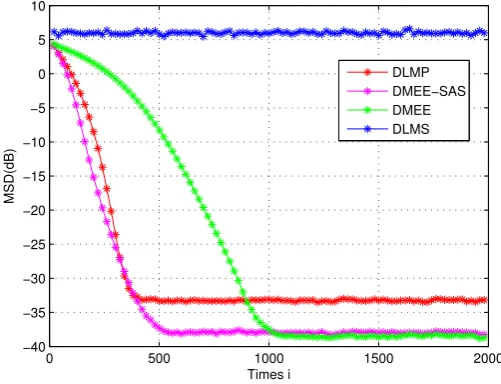
performance than the DMEE [6] algorithm when the DMEE-SAS and DMEE algorithms achieve
comparable performance.
0 500 1000 1500 2000
−40 −35 −30 −25 −20 −15 −10 −5 0 5 10
Times i
MSD(dB)
DLMP DMEE−SAS DMEE DLMS
Figure 2.Transient MSD curve. b) In non-stationary environment
Here, the simulations are carried out in the same environments as those shown in 5.1 subsection, except for the optimal estimatorw0. We compare the proposed Improving DMEE-SAS algorithm with
other algorithms.
Motivated by [14], we assume a time-varyingw0of length 6 as follows:
w0i = 1
2[a1,i,a2,i,a3,i,a4,i,a5,i,a6,i]
Whereak,i= [cos(wi+(k−21)π)]fork=1, 2, 3, 4, 5, 6 andw= 3000π .
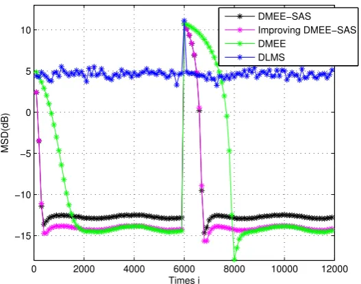
The unknown link is assume to change at time 6000. In Fig. 3, the Improving DMEE-SAS
algorithm can detect the weight vector change and the performance of it is better than DLMS
algorithm. We observe that Improving DMEE-SAS and DMEE algorithms achieve comparable
performance and Improving DMEE-SAS achieves better convergence performance than the DMEE
algorithm. When compared with DMEE-SAS algorithm, the Improving DMEE-SAS algorithm
exhibits a significant improvement in performance when the estimate near to optimal estimator. Improving DMEE-SAS algorithm achieves a low MSD and fast rate of convergence in the non-stationary environment.
0 2000 4000 6000 8000 10000 12000
−15 −10 −5 0 5 10
Times i
MSD(dB)
DMEE−SAS Improving DMEE−SAS DMEE
DLMS
Figure 3.MSD learning curves in a non-stationary environment.
5. Conclusions
In this paper, a robust diffusion estimation algorithm with self-adjusting step-size is developed
which called DMEE-SAS algorithm. The mean and mean square convergence analysis of this
new algorithm are carried out, and a sufficient condition for ensuring the stability is obtained. Simulation results illustrate that DMEE-SAS algorithm can achieve better performance than the DLMS, robust DLMP, and DMEE algorithms in non-Gaussian noise scenario. Besides, we propose the Improving DMEE-SAS algorithm using in the non-stationary scenario where the unknown parameter is changing over time. The Improving DMEE-SAS algorithm combined the DMEE-SAS WITH DMEE algorithms and it can avoid the small effective step-size of DMEE-SAS algorithm when close to the optimal estimator.
Acknowledgment
References
1. Khalil, Hassan K, Nonlinear Systems, Macmillan, New York, 1992.
2. Kong, Jun-Taek and Lee, Jae-Woo and Song, Woo-Jin, Diffusion LMS algorithm with multi-combination for distributed estimation over networks. IEEE, 2013 Asilomar Conference on Signals, Systems and Computers, 2013: 438-441.
3. Xiao, Lin and Boyd, Stephen, Fast linear iterations for distributed averaging. Systems & Control Letters, 2004, 53(1): 65-78.
4. Chouvardas, Symeon and Slavakis, Konstantinos and Theodoridis, Sergios, Adaptive robust distributed learning in diffusion sensor networks. IEEE Transactions on Signal Processing, 2011, 59(10): 4692-4707. 5. Wen, F., Diffusion least-mean P-power algorithms for distributed estimation in alpha-stable noise
environments. Electronics Letters, 2013, 49(21): 1355-1356.
6. Li, Chunguang and Shen, Pengcheng and Liu, Ying and Zhang, Zhaoyang, Diffusion information theoretic learning for distributed estimation over network. IEEE Transactions on Signal Processing, 2013, 61(61): 4011-4024.
7. Cattivelli, Federico S and Sayed, Ali H, Diffusion LMS strategies for distributed estimation. IEEE Transactions on Signal Processing, 2010, 58(3): 1035-1048.
8. Han, Seungju and Rao, Sudhir and Erdogmus, Deniz and Jeong, Kyu-Hwa and Principe, Jose, A minimum-error entropy criterion with self-adjusting step-size (MEE-SAS). Signal Processing, 2007, 87(11): 2733-2745.
9. Arablouei, Reza and Werner, Stefan and Do ˘gançay, Kutluyıl, Analysis of the gradient-descent total least-squares adaptive filtering algorithm. IEEE Transactions on Signal Processing, 2014, 62(5): 1256-1264. 10. Kelley, C. T., Iterative methods for optimization. SIAM, Philadelphia. J.appl.probab, 1999, 9: 878-878. 11. Sayed, AH, Adaptive Filters. Hoboken. NJ: John Wiley & Sons, 2008.
12. Chen, Jianshu and Sayed, Ali H, Diffusion adaptation strategies for distributed optimization and learning over networks. IEEE Transactions on Signal Processing, 2012, 60(8): 4289-4305.
13. Sayin, Muhammed O and Vanli, N Denizcan and Kozat, Suleyman Serdar, A novel family of adaptive filtering algorithms based on the logarithmic cost. IEEE Transactions on Signal Processing, 2014, 62(17): 4411-4424.
14. Zhao, Xiaochuan and Tu, Sheng-Yuan and Sayed, Ali H, Diffusion adaptation over networks under imperfect information exchange and non-stationary data. IEEE Transactions on Signal Processing, 2012, 60(7): 3460-3475.
15. Lopes, Cassio G and Sayed, Ali H, Incremental adaptive strategies over distributed networks. IEEE Transactions on Signal Processing, 2007, 55(8): 4064-4077.
16. Rabbat, Michael G and Nowak, Robert D, Quantized incremental algorithms for distributed optimization. IEEE Journal on Selected Areas in Communications, 2005, 23(4): 798-808.
17. Nedic, Angelia and Bertsekas, Dimitri P, Incremental subgradient methods for nondifferentiable optimization. SIAM Journal on Optimization, 2001, 12(1): 109-138.
18. Kar, Soummya and Moura, José MF, Distributed consensus algorithms in sensor networks with imperfect communication: Link failures and channel noise. 2009, 57(1): 355-369.
19. Cattivelli, Federico S and Sayed, Ali H, Diffusion strategies for distributed Kalman filtering and smoothing. 2010, 55(9): 2069-2084.
20. Middleton, David, Non-Gaussian noise models in signal processing for telecommunications: new methods an results for class A and class B noise models. IEEE Transactions on Information Theory, 1999, 45(4): 1129-1149.
21. Zoubir, Abdelhak M and Koivunen, Visa and Chakhchoukh, Yacine and Muma, Michael, Robust estimation in signal processing: A tutorial-style treatment of fundamental concepts. IEEE Signal Processing Magazine, 2012, 29(4): 61-80.
22. Zoubir, Abdelhak M and Brcich, Ramon F, Multiuser detection in heavy tailed noise. Digital Signal Processing, 2002, 12(2): 262-273.
24. Zhao, Xiaochuan and Tu, Sheng-Yuan and Sayed, Ali H, Diffusion adaptation over networks under imperfect information exchange and non-stationary data. IEEE Transactions on Signal Processing, 2012, 60(7): 3460-3475.
25. Carli, Ruggero and Chiuso, Alessandro and Schenato, Luca and Zampieri, Sandro, Distributed Kalman filtering based on consensus strategies. IEEE Journal on Selected Areas in Communications, 2008, 26(4): 622-633.
26. Li, Hualiang and Li, Xi-Lin and Anderson, Matthew and Adali, Tülay, A class of adaptive algorithms based on entropy estimation achieving CRLB for linear non-Gaussian filtering. IEEE Transactions on Signal Processing, 2012, 60(4): 2049-2055.
27. Cattivelli, Federico S and Lopes, Cassio G and Sayed, Ali H, A diffusion RLS scheme for distributed estimation over adaptive networks. 2007 IEEE 8th Workshop on Signal Processing Advances in Wireless Communications, 2007, 1-5.
28. Abadir, Karim M and Magnus, Jan R, Matrix algebra. Cambridge University Press, 2005, 1.
29. Shen, Pengcheng and Li, Chunguang, Minimum Total Error Entropy Method for Parameter Estimation. IEEE Transactions on Signal Processing, 2015, 63(15): 4079-4090.
c