Digital Image Transformation
and Compression
A Thesis submitted for examination for the Degree
of Master of Engineering (Electrical)
By
E. Lenc
B. Eng (Elec.)
Victoria University of Technology
Department of Electrical and Electronic Engineering
Victoria University of Technology
P.O. Box 14428, M C M C ,
Melbourne, Victoria 8001,
Australia
FTS THESIS
621.367 LEN
30001005127008
Lenc, Emil
Statement of Originality
I, Emil Lenc, hereby declare that this submission is m y o w n work and that, to the best
of my knowledge, it contains no material previously published or written by another
person nor material which to a substantial extent has been accepted for the award of
any other degree or diploma of a university or other institute of higher learning, except
where due acknowledgment is made in the text.
Uv
Table of Contents
Table of Contents i
List of Figures v
List of Tables viii
Abstract x
Acknowledgments xii
Abbreviations xiii
1. Introduction 1-1
2. Research Background 2-1
2.1 Introduction 2-1 2.2 Lossless Compression Techniques 2-2
2.2.1 Run-Length Coding 2-3 2.2.2 Statistical Coding 2-3 2.2.3 Differential Pulse Code Modulation ( D P C M ) 2-4
2.3 Lossy Compression Techniques 2-5
2.3.1 Subsampling 2-5 2.3.2 Transform Coding 2-6
2.3.2.1 Kahrunen Loeve Transform 2-7 2.3.2.2 Discrete Cosine Transform 2-7
2.3.2.3 Fractal Transform 2-8 2.4 Interframe Compression Techniques 2-9
2.4.1 Introduction 2-9 2.4.2 Predictive 2-9
2.4.3 Interpolative 2-10 2.4.4 Motion Prediction 2-10 2.5 Colour Space Transformation 2-10
2.5.1 Introduction 2-10 2.5.2 Quantisation 2-11 2.5.3 Subsampling 2-11 2.6 C o m m o n Compression Standards 2-12
2.6.1 J P E G (Joint Photographic Experts Group) 2-12 2.6.2 M P E G (Moving Picture Experts Group) 2-13
3. Outline of Research 3-1
3.2.2 Specific A i m s 3-1
3.3 Basic Structure of Algorithm 3-2
3.3.1 The Compression Process 3-3
3.3.2 The Decompression Process 3-4
3.4 Testing Platform 3-5
3.5 Test Procedure 3-6
3.5.1 Error Measurements 3-6
3.5.2 Timing Benchmarks 3-8 3.5.3 Entropy Measurements 3-8
3.5.4 Output Data Size 3-8
3.6 The Image Test Set 3-9
3.6.1 Standard Images 3-9 3.6.2 Supplementary Images 3-10
3.6.3 Image Data Format 3-11
4. The Discrete Cosine Transform 4-1
4.1 Introduction 4-1
4.2 The One-Dimensional D C T 4-2 4.3 The Two-Dimensional D C T 4-6
4.3.1 The Two-Dimensional DCT-II 4-6 4.3.2 The Two-Dimensional IDCT-II 4-6
4.3.3 Basis Functions of the Two-dimensional D C T 4-7
4.4 Factors Affecting Compression After Transformation 4-8
4.4.1 The D C T Block Size 4-8
4.4.2 Quantisation of D C T Coefficients 4-11
4.4.2.1 Visual Importance of the Coefficients 4-11 4.4.2.2 Errors Introduced Through Quantisation 4-12
4.4.2.3 Entropy Improvements Through Quantisation 4-13
4.5 Pre-processing 4-14 4.5.1 Input Data Ordering 4-15
4.5.2 Biasing 4-16
4.6 The Software Implementation 4-17 4.6.1 The Forward Transform 4-17
4.6.2 The Inverse Transform 4-21
4.7 The Hardware Implementation 4-21
4.7.1 The SGS-Thomson S T V 3 2 0 0 4-21
4.7.2 The I B M Hardware D C T Interface Description 4-22
4.7.3 The Driver for the Interface 4-24
4.7.3.1 Driver Initialisation 4-25
4.7.3.2 The Hardware Forward D C T 4-25
4.7.3.3 The Hardware Inverse D C T 4-26
4.7.3.4 Problems Associated With the Hardware D C T 4-27
4.8 Post-Processing 4-28
4.8.1 Bias Removal 4-28
4.8.2 Re-Ordering 4-28
4.9.2 Timing Benchmarks 4-31
4.9.3 Entropy Effects 4-32
4.10 Conclusion to the Chapter 4-33
5. The Quantiser 5-1
5.1 Introduction 5-1
5.2 The D C T Coefficient Properties 5-2 5.2.1 Numerical Properties 5-2
5.2.2 Functional Properties 5-8
5.3 Quantisation Effects O n D C T Coefficients 5-10 5.3.1 Error Effects O n the Reconstructed Image Data 5-10
5.3.2 Numerical Effects of Quantisation 5-15
5.4 J P E G Quantiser 5-19
5.5 Development in the Compression Algorithm 5-22
5.6 Quantiser Realisation 5-23
5.7 Results 5-27 5.7.1 Frequency Distribution 5-27
5.7.2 Reconstruction Error 5-28 5.7.3 Timing Benchmarks 5-30
5.7.4 Entropy Effects 5-30 5.8 Conclusion to the Chapter 5-32
6. The Run-Length Coder 6-1
6.1 Introduction 6-1
6.2 A Basic Run-Length Coder 6-1
6.3 The D C Coefficients 6-4
6.4 Input Statistics 6-6 6.5 Input Ordering 6-10
6.6 Run-Length Coder Design 6-12
6.7 Results 6-16
6.7.1 Timing Benchmarks 6-16 6.7.2 Entropy Effects 6-16
6.8 Conclusion to the Chapter 6-17
7. The Statistical Coder 7-1
7.1 Introduction 7-1
7.2 The Huffman Coder 7-3
7.2.1 The Fixed Huffman Coder 7-6
7.2.2 The Adaptive Huffman Coder 7-8
7.3 The Arithmetic Coder 7-9
7.3.1 Fixed 7-12
7.3.2 Adaptive 7-13
7.4 Results 7-14
7.4.1 Image Size 7-14
7.4.2 Timing Benchmarks 7-16
8. Algorithm Performance 8-1
8.1 Introduction 8-1 8.2 Compressed Image Size 8-2
8.3 M S E Levels Introduced By the Algorithms 8-4
8.4 Timing Benchmarks 8-5
9. Conclusions 9-1
9.1 Discussion of the Project 9-1
9.1.1 Project Aims 9-1
9.1.2 Algorithm Disadvantages 9-3 9.1.3 Algorithm Advantages 9-3
9.2 Suggestions For Future Work 9-4 9.2.1 Adapting the Algorithm For a Different Platform 9-4
9.2.2 Adapting the Algorithm For Motion Pictures 9-5
9.2.3 Adapting the Algorithm For Colour Images 9-5
10. Bibliography 10-1
Appendix A Image Test Set A-1
Standard Images (512x512) A-1
Standard Images (256x256) A-15
Supplementary Images A-23
Appendix B Software DCT Algorithm B-1
Software D C T Header File-DCT.H B-1 Software D C T Source File - DCT.C B-2
Appendix C Hardware DCT Interface C-1
Schematic Diagram of STV3200 Interface C-1 I B M Decoder Contents for STV3200 Interface C-2
STV3200 Driver Header File - HDCT.H C-3
STV3200 Driver Source File - HDCT.C C-4
Appendix D Algorithm Software D-1
WTNDCT.DEF - Definition File D-1
W T N D C T . R C - Resource File D-2
WINDCT.CPP - Main Program D-3
Huffman Coder - Fixed D-21
Huffman Coder - Adaptive D-23 Arithmetic Coder - Fixed D-26
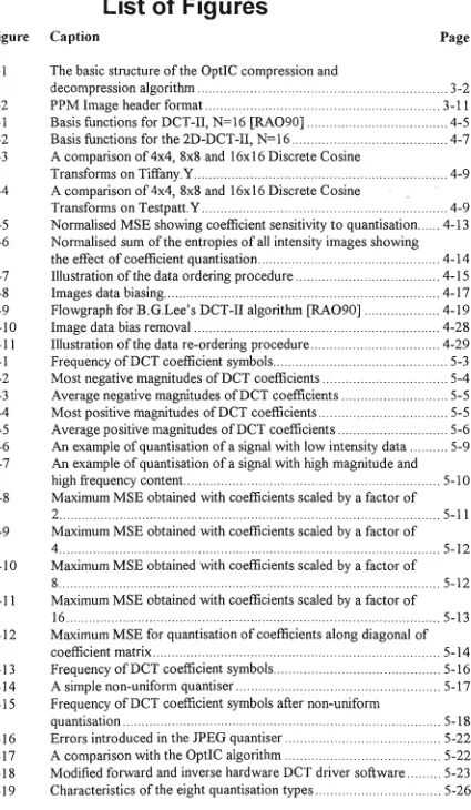
List of Figures
Figure Caption Page3-1 The basic structure of the OptIC compression and
decompression algorithm 3-2 3-2 P P M Image header format 3-11 4-1 Basis functions for DCT-II, N = 1 6 [ R A O 9 0 ] 4-5
4-2 Basis functions for the 2D-DCT-II, N = l 6 4-7
4-3 A comparison of 4x4, 8x8 and 16x16 Discrete Cosine
Transforms on Tiffany.Y 4-9 4-4 A comparison of 4x4, 8x8 and 16x16 Discrete Cosine
Transforms on Testpatt.Y 4-9 4-5 Normalised M S E showing coefficient sensitivity to quantisation 4-13
4-6 Normalised sum of the entropies of all intensity images showing
the effect of coefficient quantisation 4-14 4-7 Illustration of the data ordering procedure 4-15
4-8 Images data biasing 4-17 4-9 Flowgraph for B.G.Lee's DCT-II algorithm [ R A O 9 0 ] 4-19
4-10 Image data bias removal 4-28 4-11 Illustration of the data re-ordering procedure 4-29
5-1 Frequency of D C T coefficient symbols 5-3 5-2 M o s t negative magnitudes of D C T coefficients 5-4
5-3 Average negative magnitudes of D C T coefficients 5-5 5-4 M o s t positive magnitudes of D C T coefficients 5-5 5-5 Average positive magnitudes of D C T coefficients 5-6
5-6 A n example of quantisation of a signal with low intensity data 5-9 5-7 A n example of quantisation of a signal with high magnitude and
high frequency content 5-10 5-8 M a x i m u m M S E obtained with coefficients scaled by a factor of
2 5-11 5-9 M a x i m u m M S E obtained with coefficients scaled by a factor of
4 5-12
5-10 M a x i m u m M S E obtained with coefficients scaled by a factor of
8 5-12 5-11 M a x i m u m M S E obtained with coefficients scaled by a factor of
16 5-13 5-12 M a x i m u m M S E for quantisation of coefficients along diagonal of
coefficient matrix 5-14 5-13 Frequency of D C T coefficient symbols 5-16
5-14 A simple non-uniform quantiser 5-17
5-15 Frequency of D C T coefficient symbols after non-uniform
quantisation 5-18 5-16 Errors introduced in the J P E G quantiser 5-22
5-17 A comparison with the OptIC algorithm 5-22
5-18 Modified forward and inverse hardware D C T driver software 5-23
5-20 Frequency of D C T coefficient symbols after quantisation 5-28
6-1 A typical sequence of symbols 6-1 6-2 A run-length coded sequence - technique 1 6-2
6-3 A run-length coded sequence - technique 1 6-3
6-4 Probability of a zero symbol value for each coefficient 6-6
6-5 A n example using the J P E G ordering method 6-7 6-6 A n example using the OptIC ordering method 6-8 6-7 N u m b e r of runs per given coefficient symbol in image test set 6-13
7-1 Symbols frequencies for the run-length coded images 7-2
7-2 A sample Huffman coding process [HUF52] 7-5 7-3 Arithmetic coded example for the sequence {E, A, I, I, !}
[WIT87] 7-10 A-1 Airplane. Y original image A-1
A-2 Airplane.Y reconstructed image A-2
A-3 Baboon.Y original image A-3 A-4 B a b o o n Y reconstructed image A-4
A-5 Lena.Y original image A-5 A-6 Lena.Y reconstructed image A-6
A-7 Peppers.Y original image A-7 A-8 PeppersY reconstructed image A-8
A-9 Sailboat.Y original image A-9 A-10 Sailboat.Y reconstructed image A-10
A-ll Splash.Y original image A-ll A-12 SplashY reconstructed image A-12
A-13 Tiffany Y original image A-13 A-14 Tiffany.Y reconstructed image A-14 A-15 Beansl Y original image A-15 A-16 Beansl Y reconstructed image A-15 A-17 B e a n s 2 Y original image A-16 A-18 Beans2.Y reconstructed image A-16
A-19 Couple.Y original image A-17 A-20 C o u p l e Y reconstructed image A-17
A-21 Girll.Y original image A-18 A-22 Girll.Y reconstructed image A-18
A-23 Girl2.Y original image A-19 A-24 Girl2.Y reconstructed image A-19 A-25 GirD.Y original image A-20
A-26 GirB.Y reconstructed image A-20 A-27 House.Y original image A-21
A-28 House Y reconstructed image A-21
A-29 Tree.Y original image A-22 A-30 Tree.Y reconstructed image A-22
A-31 Testpatt.Y original image A-23 A-32 Testpatt.Y reconstructed image A-24
A-33 Wendyl.Y original image A-25 A-34 Wendyl.Y reconstructed image A-26
A-37 Wendy3.Y original image A-29
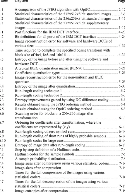
List of Tables
Table Caption Page
2.1 A comparison of the JPEG algorithm with OptIC 2-12
3.1 Statistical characteristics of the 512x512x8 bit standard images 3-9 3.2 Statistical characteristics of the 256x256x8 bit standard images 3-10
3.3 Statistical characteristics of the 512x512x8 bit supplementary
images 3-10 4.1 Port functions for the I B M D C T interface 4-23
4.2 Bit definitions for all ports of the I B M D C T interface 4-24 4.3 Image reconstruction error for software and hardware D C T s of
various sizes 4-30 4.4 Time required to complete the specified cosine transform with
block size of 4x4, 8x8 and 16x16 4-31 4.5 Entropy of the image before and after using the software and
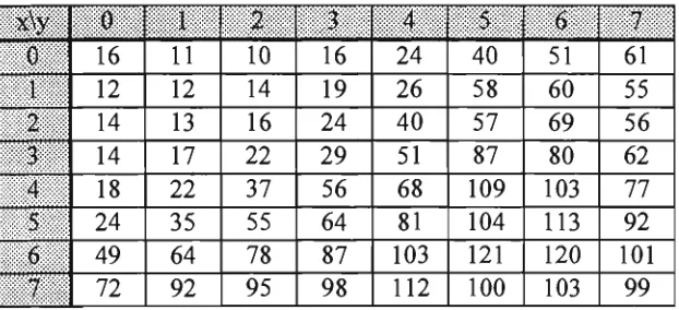
hardware D C T 4-33 5.1 Atypical J P E G quantisation matrix [ P E N 9 0 ] 5-20
5.2 Coefficient quantisation types 5-25 5.3 Image reconstruction error for the non-uniform and J P E G
quantiser 5-29 5.4 Entropy of the image after quantisation 5-31
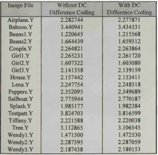
6.1 Run-length coding technique 1 6-2 6.2 Run-length coding technique 2 6-3 6.3 Entropy improvements gained by using D C difference coding 6-5
6.4 Results obtained using the J P E G ordering method 6-8
6.5 Results obtained using the OptIC ordering method 6-9 6.6 Scanning order for blocks in a 256x256 image after
transformation 6-11 6.7 Ordering for coefficients after transformation, where the
coefficients are represented by (x,y) 6-11 6.8 Run-length coding of zero symbol runs 6-14
6.9 Run-length coding of short runs of highly probable symbols 6-14
6.10 Run-length codes for large runs 6-14 6.11 Entropy of image data after run-length coding 6-17
7.1 Step by step definition of a H u f f m a n code 7-4 7.2 Huffman codes for the sample symbols 7-5 7.3 A sample probability distribution 7-9 7.4 Image sizes after compression using various statistical coders 7-14
7.5 Image sizes after compression 7-15
7.6 Times for the full compression of the images using various
statistical coders 7-16 7.7 Times for the full decompression of the images using various
8.1 A comparison of intensity image sizes after compression with
D P C M , J P E G and the n e w algorithm
8.2 A comparison of green image sizes after compression with D P C M , J P E G and the n e w algorithm
8.3 M S E introduced after reconstruction of intensity images using D P C M , J P E G and the n e w algorithm
8.4 M S E introduced after reconstruction of green images using
Abstract
Compression algorithms have tended to cater only for high compression ratios at
reasonable levels of quality. Little work has been done to find optimal compression
methods for high quality images where no visual distortion is essential. The need for
such algorithms is great, particularly for satellite, medical and motion picture imaging.
In these situations any degradation in image quality is unacceptable, yet the resolutions
of the images introduce extremely high storage costs. Hence the need for a very low
distortion image compression algorithm.
An algorithm is developed to find a suitable compromise between hardware and
software implementation. The hardware provides raw processing speed whereas the
software provides algorithm flexibility. The algorithm is also optimised for the
compression of high quality images with no visible distortion in the reconstructed
image.
The final algorithm consists of a Discrete Cosine Transform (DCT), quantiser,
run-length coder and a statistical coder. The DCT is performed in hardware using the
SGS-Thomson STV3200 Discrete Cosine Transform. The quantiser is specially optimised
for use with high quality images. It utilises a non-uniform quantiser and is based on a
series of lookup tables to increase the rate of computation. The run-length coder is
also optimised for the characteristics exhibited by high-quality images. The statistical
coder is an adaptive version of the Huffman coder. The coder is fast, efficient, and
Test results of the n e w compression algorithm are compared with those using both the
lossy and lossless Joint Photographic Experts Group (JPEG) techniques. The lossy
JPEG algorithm is based on the DCT whereas the lossless algorithm is based on a
Differential Pulse Code Modulation (DPCM) algorithm. The comparison shows that
for most high quality images the new algorithm compressed them to a greater degree
than the two standard methods. It is also shown that, if execution speed is not critical,
the final result can be improved further by using an arithmetic statistical coder rather
Acknowledgments
I wish to express my thanks to both of my supervisors, Alec Simcock and Ann
Pleasants for their help, guidance and patience. Special thanks to Alec for his curry
nights that gave me the spice of life to carry on. His special friendship and dedication
were also a great inspiration.
Special thanks also should go to my family, in particular to Dong, his help and
experience in the field of image compression was invaluable.
Finally, I owe special thanks to my wife Wendy for her untiring support and faith in
Abbreviations
CISC Complex Instruction Set Computer.
D C T Discrete Cosine Transform.
D P C M Differential Pulse Code Modulation.
DSP Digital Signal Processing.
E P L D Electrically Programmable Logic Device.
H V S Human Visual System.
JDCT Inverse Discrete Cosine Transform.
JPEG Joint Photographic Experts Group.
K L T Kahrunen Loeve Transform.
M O S Mean Opinion Score
M P E G Moving Picture Experts Group.
M S E Mean Square Error.
OptIC An acronym for the new algorithm described in this thesis.
P C X A common run-length coding technique for compressing images on an I B M
PC.
P P M A common image format which provides no compression.
R G B Red, Green, Blue colour coding model.
RISC Reduced Instruction Set Computer.
1. Introduction
The need for image compression techniques has been apparent for many years now.
This need has lead to the design of many algorithms and many different
implementations of these algorithms. The more common of these are described in
chapter 2. Unfortunately, most of these algorithms concentrate on increasing the
compression factor rather than maintaining high-fidelity. They are generally aimed for
video or television quality images where some losses in quality can be tolerated.
During the literature survey no documentary evidence was found of research
specifically aimed at high compression rates for high quality images. The emphasis
here is to prevent the introduction of visible distortions into the image whilst still
trying to optimise the compression factor. This form of compression would be
extremely useful in applications where such levels of quality are a necessity e.g.
medical imaging, satellite imaging and cinema quality motion pictures. The images in
these applications are often of extremely high resolution and so require large storage
requirements. They also demand high quality and no distortions are acceptable as
life/death or profit/loss decisions may depend on very fine data contained within
them. However, data storage comes at a cost and any increase in compression factor
can produce a proportional decrease in storage cost.
This thesis sets out to define a high quality, high speed compression algorithm OptIC
is a necessity. Particular emphasis is placed on optimising the compression factor
whilst maintaining visible image quality.
Chapter 3 defines the aims of the project, the basic principles of the OptIC algorithm
required to achieve these aims and how the algorithm will be tested to ensure that the
aims have been fulfilled. Chapters 4 to 7 explain the functional components of the
algorithm in further detail. Each of the functional components are described in detail.
They are then tested as part of a stepwise refinement and conclusions made at the end
of each chapter describing the effectiveness of the implementation of the OptIC
algorithm to that point. Chapter 8 takes the entire algorithm and compares it with
currently existing algorithms to measure its overall performance.
A final conclusion and discussion of the advantages and disadvantages may be found
in chapter 9. This chapter also introduces some research avenues that may be pursued
2. Research Background
2.1 Introduction
Digital image compression provides a means by which the storage requirements of a
digitised image may be reduced with little or no reduction in quality. This is done by
removing redundancies which may occur within the image. Consider a typical motion
picture frame with a resolution of 6000 by 4000 pixels (picture elements) each with a
colour resolution of 24 bits allowing 16 million possible colours. A single frame of
this image requires 576 Mbits of storage. If this image was compressed by half, the
total storage costs would be halved. This would also save costs if the image was to be
transmitted in the compressed form as it could be transmitted in half the time of the
original.
A number of factors allow images to be compressed to a greater degree than other
forms of data, such as text or binary code. Firstly, image data is two-dimensional
providing correlation in two directions; this allows us to predict adjacent pixel
intensities with greater accuracy. In motion picture sequences, the data may be
considered to be three-dimensional thus providing correlation in three directions and
so further improving the prediction of adjacent pixels. Secondly, the restored image
data does not need to be exactly the same as the original image since the human eye
A n image compression algorithm is generally, though not always, composed of two
basic components: a predictive function and a symbol coding function. The predictive
function attempts to reduce the entropy of the data to be compressed; see chapter 3 for
the definition of entropy in this context. The predictor does not normally perform any
compression, it only maps the data into a different form that is more readily
compressed by the symbol coding function. The predictor can be either lossless or
lossy depending upon whether or not it introduces errors after reconstruction of the
data.
The symbol coding function generally takes the form of an entropy or statistical coder
and is the component that performs the compression. These coders are lossless and so
do not introduce any further error into the data after reconstruction. They are treated in
more detail in chapter 7.
Both lossless and lossy techniques exist to compress motion pictures and colour
images.
2.2 Lossless Compression Techniques
The term lossless implies that the coding method used is entirely circular or
reversible, i.e. the compression-decompression procedure returns the image bit for bit
to its original state. A lossless technique either has no predictor function or has a
predictor function that is lossless. In general these algorithms will compress images
It is possible to have a lossy algorithm method which m a y appear to be lossless. In this
situation the predictive component of the algorithm only introduces errors in those
areas which would not be obvious or noticed because of imperfections in the eye.
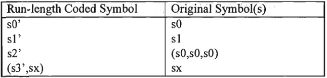
2.2.1 Run-Length Coding
Run-length coding [HUA74, THI92] is most effective in coding data which contains
large strings of the same value. It replaces large symbol strings with a shorter
run-length code. That code contains an identifier code, the run-length of the string and the data
contained within the string. The predictor of the run-length coder assumes that
adjacent pixels will most probably contain the same value. For this reason, it is
generally used for compressing cartoon-style images containing large patches of
uniform colouring. It is also useful for compressing bi-level images such as FAX
images as they often contain large areas of white space.
The compression achieved with run-length coding is not very good when it is used to
code gray-scale or colour images, particularly if the images contain noisy data or
constantly varying shades and colours. The PCX image format is a commonly used
image compression format that incorporates run-length coding.
2.2.2 Statistical Coding
Statistical or entropy coding [THI92] is useful for compressing data with large
quantities of a particular data value. This is achieved by assigning shorter codes for
values which are less probable. T h o u g h it is possible, a statistical coder is not
particularly effective when used on its own, generally providing only about 20%
compression. To be effective, it is generally performed after a predictive function.
An inherent problem of this form of coding is the need for statistical data about the
input data. Fixed coders assume a particular set of statistics for the input data but
perform poorly when the input data statistics deviate from this. Adaptive coders
generate the statistical data on the run and so adjust to varying statistical trends. Both
of these coders perform poorly when the input data is extremely noisy or random.
2.2.3 Differential Pulse Code Modulation (DPCM)
In DPCM [COR90, EKS84] the predictive stage relies on the high degree of
correlation that occurs between neighbouring pixels in an image. The prediction
algorithm attempts to predict the value of the next pixel by taking into account the
values of previous pixels. The difference of the predicted and actual pixel value is
then stored as this is typically smaller in magnitude than the actual pixel value itself.
Improved prediction may be obtained by taking into account more pixels on the
current or previous line of the image to predict the value of the next pixel with greater
accuracy. Once again, only the difference value would be stored.
The final stage of the DPCM algorithm is the coding section. Here an entropy coding
method is used to perform the actual compression. This technique, on average,
2.3 Lossy Compression Techniques
In order to obtain higher compression ratios for images, it is necessary to use lossy
compression techniques. Lossy techniques are not circular, i.e. the
compression-decompression procedure will produce distortions in the reconstructed image. This
implies that the predictor block is present and that it introduces errors into the
reconstructed image.
2.3.1 Subsampling
Subsampling [GRU92, QUI93] is a very but simple form of image compression. The
predictor simply reduces the horizontal and vertical resolutions upon compression.
For example a compression ratio of 4:1 can be achieved by reducing the horizontal
and vertical resolutions by a factor of two. The decompression process would then
need to expand each pixel into a 2x2 pixel block containing the same colour and
intensity of the sub-sampled pixel. The distortion in this case becomes apparent even
at relatively low rates of compression, as the pixel expansion tends to produce a
blocking effect.
Sophisticated subsampling techniques attempt to interpolate between the pixels of the
compressed image. This, in effect, is a form of low pass filtering and tends to soften
2.3.2 Transform Coding
Transform coding techniques are typically more computationally intensive than other
compression methods. This technique requires two steps : transformation and coding
[EKS84, AM089, BAR88, KOU89, RAB89].
The transform forms the predictor function of the algorithm and operates on a two
dimensional block of data to produce an array in which most of the image information
is stored in as few elements of the array as possible. The transformed data represents
the levels of the frequencies in the two-dimensional space within a block. The block
size of the transform ranges between 4x4 and 16x16. Block sizes smaller than this do
not produce good results and larger block sizes become computationally difficult to
calculate.
The coding stage of this method requires the selection, quantisation and storage of the
transformed data. The most significant values, i.e. those values which hold the
majority of the image information are quantised the least so as to keep their values
intact. The resulting data is then coded using similar coding techniques to those
mentioned in section 2.2.3 for predictive coding. Note that the quantisation stage
causes the distortions which may be visible after decompression.
The compression ratios obtained from transform coding are much greater than those
obtained from predictive coding. This is especially so where there is little correlation
transforms for digital image coding, such as D C T , only work well if the inter-pixel
correlation is high [CLA85]. In general there is a trade-off between the compression
ratio and the fidelity of the resulting image.
The Kahrunen Loeve Transform, Discrete Cosine Transform and the Fractal
Transform are three of the most commonly used transforms.
2.3.2.1 Kahrunen Loeve Transform (KLT)
The KLT [RAO90, STA88] is the optimum transform for image coding. It is,
however, computationally slow as no fast algorithms exist. There are a number of
related transforms which have been designed to provide a compromise between image
quality, compression ratio and computational complexity. The most common of these
is the Discrete Cosine Transform (DCT).
2.3.2.2 Discrete Cosine Transform (DCT)
The DCT [RAO90] is most frequently used for image compression. Its popularity is
due to its being a very close approximation of the KLT. There are also quite a large
number of fast algorithms available for evaluating the transform and its inverse. A
number of hardware implementations of the DCT have also become available. For
these reasons the DCT is also used in the OptIC (Optimised Image Compression)
2.3.2.3 Fractal Transform
The Fractal Transform [BAR88, SKA94, W0094] is the most recent of the three
transforms discussed here. The transform itself can produce extremely complex yet
natural looking images with only a small number of coefficients. Unfortunately the
process of obtaining the coefficients required to produce a particular image is not a
simple process. Barnsley [BAR88] invented the fractal transform and has since
brought out a number of software packages which utilise this transform in image
compression.
The fractal transform is an asymmetric algorithm, i.e. it takes a great deal longer to
compress an image than it does to decompress it. The compression time is about 48
minutes on a 33Mhz 80486-based machine for a 640x400 pixel 24 bit colour image
[DET92]. The decompression time for the same image is performed in the order of a
few seconds.
One problem with the fractal transform is the lack of any quantitative quality
measurements. There are often claims of extremely large compression ratios (75:1)
but no mention of the quality of the restored image [SAU94]. Also the algorithm is
2.4 Interframe Compression Techniques
2.4.1 Introduction
Interframe compression [EKS84, QUI93] is useful for sequences of images or motion
picture images. In most sequences of images there is a high level of redundancy in the
information between two consecutive frames, particularly when the background of the
image is constant and only the foreground varies. Interframe compression works to
reduce this redundancy. To allow motion to commence from various points in the
image sequence without decoding the entire image sequence, reference frames are
taken periodically. These reference frames form the points between which or from
which the compression will take place. The use of reference frames also prevents
continuous degradation in the image quality in a lossy algorithm which would occur if
only one reference image was taken and all subsequent images were based on this.
2.4.2 Predictive
In predictive coding [GRU92] for interframe compression, the difference between
reference frames is taken and later used to re-create the second reference frame from
the first. For images where the background is constant, the differencing will produce a
large number of zeros which are easily compressed. The predictive algorithm is
2.4.3 Interpolative
The interpolative method [GRU92, QUI93], also known as average prediction or
forward and backward prediction, calculates the current frame based on differences
between the last and the next reference frame. So, for example, only every second or
third frame could be kept and the intermediate frames would then later have to be
predicted. As this algorithm requires the average of frame information, it is a lossy
one.
2.4.4 Motion Prediction
Motion prediction [GRU92, QUI93] attempts to isolate moving objects and track their
movements across subsequent frames. More advanced algorithms may also determine
if the object has rotated or changed in scale to provide improved results in
compression. In general, these algorithms are rather complex and difficult to
implement. Also, the coding algorithm is often more complicated than the decoding
algorithm. The motion predictor often makes approximations in order to simplify the
coding procedure; this leads to losses.
2.5 Colour Space Transformation
2.5.1 Introduction
Colour space transformations provide methods of reducing redundancy in colour
images. These in general make use of characteristics of the Human Visual System
perceive intensities. The h u m a n eye is also more sensitive to certain colours than to
others. For this reason the common RGB (Red, Green, Blue) colour model is more
often transformed to the YIQ model where Y is the intensity component and I and Q
are the chrominance or colour components. The YIQ format more accurately models
the eye's capabilities. The transformation is shown in (2.1).
Y I
Q
0.299 0.587 0.114
0.596 -0.274 -0.322
0.211 -0.522 0.311
R G B
(2.1)
2.5.2 Quantisation
Quantisation of the colour space [QUI93] simply reduces the precision of the colour
carrying information. This will reduce the total number of colours that may be
represented in the image. In general, before the quantisation is performed, the colour
space is transformed to the YIQ format as described in section 2.5.1. By doing so the
colour set will still contain those colours which are most clearly identified by the
human eye and reduce redundancy. In this case the chrominance (IQ) is normally
quantised more than the intensity (Y).
2.5.3 Subsampling
Subsampling in the colour space [QUI93] averages the colours in a block of pixels
and in effect reduces the resolution of the colour image whilst leaving the resolution
2.6 Common Compression Standards
2.6.1 JPEG (Joint Photographic Experts Group)
The JPEG algorithm [QUI93] defines methods for coding still picture images using
both lossless and lossy techniques. The lossless technique is based on predictive
coding as described in section 2.2.3. The lossy technique is based on the discrete
cosine transform (DCT) and a combination of run-length and statistical coding. The
DCT is an 8x8 DCT and is performed on each of the three colour channels.
The algorithm has been implemented on a variety of systems and is available in
software and hardware versions. The implementations range from low cost, low
performance systems to high cost, high performance systems.
Although this algorithm is capable of producing high quality reproductions of images
after compression it is not optimised for this purpose. Instead, it is aimed at the
average consumer market where high rates of compression rates are preferred to high
quality.
Feature
D C T Block Size
Coefficient Ordering
Block Ordering
Grouping
Compression Stage
J P E G
8x8.
Zig-Zag.
Left to right.
Coefficients in same
block grouped.
A run-length coder
stage only.
OptIC
16x16.
Proportional to the coefficients
probability of being zero.
Alternating left to right then
right to left.
Like coefficients grouped.
A run-length and statistical
coder stage.
A s the OptIC algorithm is also based on the D C T it is useful to see h o w it differs from
the JPEG algorithm. The major differences are briefly highlighted in Table 2.1. •
2.6.2 MPEG (Moving Picture Experts Group)
The MPEG algorithm [FAI95, QUI93, THI92] is an extension of the lossy techniques
outlined in the JPEG algorithm. It defines a standard for coding moving pictures with
a sound track. The MPEG does not precisely detail the procedure for compressing
video images as does JPEG; it merely specifies the format and data rate of the output
bitstream as well as a set of compression techniques that can achieve varying degrees
of quality. MPEG uses JPEG for the intraframes together with combinations of both
predictive and interpolated motion compensation and sub-band coding for the audio.
As the MPEG standard only specifies the output format, most of the products
currently on the market only perform MPEG decompression. Only three real-time
high quality encoders existed by July 1995 [GIL95]. As with JPEG, MPEG is already
available in both software and hardware implementations. Recently (July 1995), both
SGS-Thomson Microelectronics and Zatek introduced MPEG decoders for decoding
both video and audio.
The output quality of the MPEG algorithm is relatively poor as it is optimised for high
speed and high levels of compression rather than for quality. For this reason it is not
3. Outline of Research
3.1 Introduction
An outline of the research aims is to be presented together with a proposed algorithm
structure to realise these aims. A test platform and a set of test methods are also
defined. These provide a means to determine whether or not the set aims have been
achieved.
3.2 Research Aims
3.2.1 General Aims
The aim of this research is to compress motion picture quality images using an
optimal combination of hardware and software to minimise costs and maximise
performance. Most compression systems are either fully software based and require
extremely high performance computers to provide any reasonable performance
[GRU92, KOU89, CHA87] or they are fully hardware based and suffer from high
costs and inflexibility [LE093, TSA89, ART88, STA88, REZ87].
3.2.2 Specific Aims
• To transform digitised images into a format more suitable for manipulation using
computers, and then to reduce the amount of information required to represent the
original optical impression by at least a factor of 2, whilst maintaining fidelity of
• T o store and retrieve an image, and to reconstitute the original optical image from
the stored information.
• To produce compression and reconstitution algorithms that are adaptable for use in
processing motion picture quality images (approx. 6000x4000x24 bits) in the order
of five seconds with a minimum reduction of image quality. Initially, smaller
images will be used (256x256x8 bits or 512x512x8 bits); all results will then be
extrapolated for the full resolution.
• To investigate various transformation and compression techniques.
• To choose and optimise a compression / transform technique for use in a hardware
/ software implementation.
3.3 Basic Structure of OptIC Algorithm
The basic structure of the OptIC (Optimised Image Compression) algorithm is shown
in Fig. 3-1. It can be seen from this diagram that the compression and decompression
components of the OptIC algorithm are each composed of six distinct functions.
T h e Compression Pre-processing
T h e Decompressi Statistical Decoding — •
Process:
— >
on 1
Forward
DCT
'rocess: Run-length
Decoding — •
Quantisation
Re-ordering — • — •
Ordering —1
Run-length * Coding
De-quantisation Inverse -* DCT — •
—>
Statistical Coding
Post-processing
3.3.1 T h e Compression Process
The pre-processing block conditions the input image data so that it is in a format
readily accepted by the forward DCT function. The pre-processing also adds a bias to
the image data so that the average of the image data lies approximately about the zero
value. This block does not add any error to the data nor does it in any way affect the
entropy of the original image data.
The forward DCT function transforms the image data and outputs an array of DCT
coefficients. The number of coefficients output is equivalent to the number of pixels
in the input image. As these coefficients are twice the precision of the pixel data in the
original image, this block actually doubles the storage requirement of the image. It
does, however, improve the entropy of the image and so the image can be compressed
to a greater extent than the original image by a statistical coder. The DCT process
introduces an extremely small amount of error to the image data and so forms the first
lossy function.
Once the image has been transformed it is then quantised to reduce the precision of
the coefficients which do not have a great affect on our perception of the image. This
improves the entropy yet again but in the process also increases the error introduced
into the image data and as such, it forms the second lossy function. The errors
introduced here, though much greater than those introduced in the DCT process, are
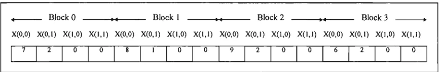
T h e effect of quantisation o n the image tends to reduce a n u m b e r of coefficients to
zero. By ordering the coefficients produced by the DCT, it is possible to increase the
chance of generating large lengths of zero values. These can then be effectively
compressed by the run-length coder.
The run-length coder function replaces repetitions of a like value with one or two
smaller values. This effectively is the first compression function in the algorithm and
is completely lossless. As the run-length coder looks at the relationship between
neighbouring values, it can produce better results when used in conjunction with a
statistical coder than those obtained by using the latter alone.
The run-length coded data is finally passed through a statistical coder which forms the
second and final compression function in the algorithm. The statistical coder is also a
lossless coder which looks at the statistics of the data and replaces frequently
occurring data symbols with short symbols and less frequently occurring data symbols
with longer symbols.
3.3.2 The Decompression Process
The decompression process is basically the exact reverse of the compression process.
The compressed image data is first statistically decoded to produce the run-length
coded data that is then passed through the run-length decoder to produce the ordered
and quantised DCT coefficients. These coefficients are re-ordered back to their
original positions and then de-quantised to approximate the original coefficient values
the original quantisation function, the values of the coefficients that are output from
the de-quantiser are only an approximation of those that were originally produced by
the forward DCT process.
Once the coefficients have been restored they are passed through the inverse DCT.
This function will add further error though in this process it is very minute. The
output of the inverse DCT is finally passed through the post-processing function that
removes the bias that was introduced by the pre-processing function. The final output
will be, apart from the introduced errors, the reconstructed version of the original
image. The accumulated errors obtained throughout the entire compression and
decompression process are not visible to the human eye.
3.4 Testing Platform
All of the tests were performed on an IBM compatible computer based on the
80486SX processor running at a clock speed of 33 MHz (this does not include a
floating point processor). The computer was equipped with 8 Mb of memory, 410 Mb
Hard disk and 256 Kb of cache memory. The hard disk was controlled by a standard
VESA local bus IDE hard disk controller card. A Cirrus Logic VL-VGA-24 graphics
card fitted with 1 Mb of VRAM was used. It is common practice to use a Sony Grade
1 monitor for subjective evaluation exercises; but as one was not available, an NEC
Multisync 4D monitor in True colour mode (24 bit per pixel or 16 million colours) was
The software for the OptIC algorithm w a s developed using a Borland C + + Compiler
version 4.0 for Microsoft Windows. The algorithm was executed under Microsoft
Windows version 3.1.
3.5 Test Procedure
Where applicable four important tests were performed after the introduction of each
function to measure progress and to provide a progressive indication of the
performance of the compression algorithm. These four tests are : measuring the error
introduced by a lossy function, the timing benchmarks with the function included, the
entropy of the data after introduction of a function and the size of the output data after
introduction of a compression function.
3.5.1 Error Measurements
A number of error measurement techniques exist, the most common of these is the
Mean Square Error (MSE) as defined in (3.1) [RAO90] for an NxM image where
x(m,n) is an element in the original image and x(m,n) is an element in the
reconstructed image.
i M-\ N-\ 2
This form, though very commonly used, does not incorporate the Human Visual
System (HVS) and so does not provide a real indication of how much of the error the
A number of attempts have been m a d e to define a method of measuring error which
would be perceived by the human eye [HOS86, MIY85] but these methods are not
entirely accurate and it has not been proved that they apply for all types of images. As
such they would not form a reliable method of testing the image quality. Instead a
form of Mean Opinion Score (MOS) was devised. Images were subjected to
increasing levels of compression and the image qualities verified by individual
inspection at very close distances from the monitor screen. The image inspection was
performed by a group of ten randomly chosen university students, three staff
members, five family members and myself. The group consisted of a wide spread of
ages and technical ability, all individuals had to decide whether or not they could
perceive any differences between the original image and the reconstructed image. The
image on the display could be quickly swapped between original and reconstructed
image so that any distortions may be easily observed. In order to satisfy the aims ail
the individuals had to agree that all of the images contained no visible distortions after
reconstruction. A note was made (for both the JPEG and OptIC algorithms) of the
greatest compression which each image could tolerate with no observer identifying
errors. This represents a subjective mean opinion score of the algorithm's capability to
compress without introducing visible errors (please see section 8.3 and Tables 8.3 and
3.5.2 Timing B e n c h m a r k s
In all of the test cases the test was executed ten times and timed using a stop-watch.
The result was then divided by ten giving a result that is at least accurate to the nearest
tenth of a second.
3.5.3 Entropy Measurements
The measurement of entropy gives an indication of how much further an image may
be compressed if processed with an ideal statistical coder. It is thus an important test
in determining the effectiveness of processes that only manipulate data but do not
actually compress it, such as, the DCT and the quantisation processes. The entropy of
an image can be defined by (3.2) where N is the number of symbols and p(i) is the
probability of the i symbol.
N
Entropy = - ^ p(i) log2 p(i) (3.2)
The entropy value is the average number of bits required to code each of the possible
symbols. This implies that a reduction in entropy would result in a smaller output data
size if the data was to be passed through a statistical coder.
3.5.4 Output Data Size
The output data size of the image after processing is simply the size of the data when
3.6 The Image Test Set
3.6.1 Standard Images
Fifteen standard images were used to form the standard image test set. These are
images which are commonly used for testing image compression algorithms and
provide a base from which the algorithm may be compared with other existing
algorithms. The images were originally stored as colour images that were converted to
intensity images and green component images as these were the components generally
used by other compression techniques for comparison. The statistical characteristics
for the 512x512x8 and the 256x256x8 bit pixel images are tabulated in Tables 3.1,
and 3.2 respectively. A hard copy of each of the intensity images, both original and
reconstructed, can be found in Appendix A.
Image airplane airplane baboon baboon lena lena peppers peppers sailboat sailboat splash splash tiffany tiffany Image
T y p e
-Intensity Green Intensity Green Intensity Green Intensity Green Intensity Green Intensity Green Intensity Green average 179.132 177.856 129.694 128.863 124.108 99.056 120.464 115.581 125.284 124.305 103.284 70.521 211.345 208.631 variance 2161.472 2687.813 1789.110 2282.638 2298.224 2796.058 2909.980 5629.022 4297.523 6026.763 2662.172 3638.671 862.075 1125.752
m i n i m u m
16
0
0
0
25
1
0
0
2
0
9
0
0
0
m a x i m u m
231
234
231
236
245
248
228
237
239
249
242
247
255
255
entropy 6.705764 6.805543 7.358139 7.475280 7.447764 7.595153 7.594303 7.518362 7.485789 7.646107 7.258475 6.916109 6.600483 6.689978Image beansl beansl beans2 beans2 couple couple girll girll girl2 girl2 girl3 girl3 house house tree tree Image Type Intensity Green Intensity Green Intensity Green Intensity Green Intensity Green Intensity Green Intensity Green Intensity Green average 176.000 180.638 167.403 170.869 33.424 30.122 58.872 139.960 139.691 139.960 111.114 99.275 138.066 133.004 129.115 124.906 variance 1469.183 2021.443 1849.728 2562.536 1000.177 989.483 1579.841 857.937 880.510 857.937 2471.922 2871.558 2128.970 3145.283 4554.317 5854.357
m i n i m u m
32
19
24
9
1
0
1
30
27
30
14
0
16
0
0
0
m a x i m u
m
204
212
207
213
244
254
234
255
255
255
250
254
240
246
237
238
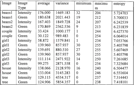
entropy 5.724703 5.700033 6.242539 6.231839 6.427370 6.064014 7.053766 5.405798 5.607469 5.405798 7.261685 7.325684 6.504477 6.551604 7.314443 7.418101Table 3.2 Statistical characteristics of the 256x256x8 bit standard images.
3.6.2 Supplementary Images
A number of supplementary images were also generated to support the test set. The first
of these images, testpatt, was generated by a C program to test the compression
algorithms ability to compress various frequencies of alternating low and high intensity.
Image testpatt wendyl wendy2 wendy2 wendy3 wendy3 Image Type intensity intensity intensity green intensity green average 112.026 155.573 65.610 68.916 109.056 107.081 variance 16016.361 7239.374 3881.104 4113.347 4813.107 5252.605 minimu m
0
1
1
0
0
0
m a x i m u
m
255
255
255
255
253
255
entropy 0.989348 6.822758 7.096842 6.544705 7.821364 6.820176The remaining images were obtained from photographs digitised using a high
resolution Hewlett Packard colour image scanner. All of the images were 512x512x8
bits, and their characteristics are shown in Table 3.3. A hard copy of each intensity
image, both original and reconstructed, can be found in Appendix A.
3.6.3 Image Data Format
All of the images are stored in format known as the PPM format. This format is used
because the data is stored in a raw format with no compression. This format is also
quite simple and so it is very easy to read.
The PPM file consists of a header which identifies the image format and also provides
information about the width, height and the maximum intensity of the pixels.
Following the header is the raw image data where each byte represents a pixel
intensity and the pixels are stored consecutively on a line by line basis.
The image header format is shown in Fig. 3-2 where LF is the code for a line-feed
(decimal 10) and the width, height and maximum intensity are ISO-coded values. An
ISO-coded value is simply the required number stored with a separate character for
each digit in that value. For example, the number 134 when stored in an ISO-coded
format would become the characters {"1", "3", "4"}.
"P" "5" LF Width CC 5?
Height LF M a x i m u m Intensity LF
The software to read and write a P P M format image m a y be found in Appendix D.
The C functions for the read and write are Loadlmage (page D-ll) and
4. The Discrete Cosine Transform
4.1 Introduction
The original Discrete Cosine Transform (DCT) is based on the Fast Fourier Transform
(FFT) [RAO90, WAN84]. Since its discovery in 1974 [AHM74], its use has become
widespread in digital signal processing (DSP), in particular for image processing.
There are a number of reasons for its popularity, the DCT is real, separable,
orthogonal and it approaches the statistically optimal transform, KLT [KAR47,
LOE60]. The DCT does not suffer the computational problems involved in generating
the KLT, as it is not dependent on signal statistics. Furthermore there are a large
number of fast algorithms available to evaluate the DCT [LEE84, WAN84, SUE86,
CHA87, KOU89]; a number of these have also been implemented in hardware for
extremely high speed processing [JUT87, REZ87, ART88, QUI93, LE093]. As the
DCT is a separable transform, it is also possible to extend all the algorithms to
multiple dimensions.
The DCT forms the heart of the image compression algorithm described in this thesis.
The transform does not actually compress the data. It could instead increase the size of
the data since the resolution of the output coefficients is generally greater than that of
the input data. It does, however, have the useful property of reducing the entropy of
the input data. The entropy of the data gives an indication to the extent of which an
compressible. This is achieved by transferring the majority of the input vector
information or energy into small number of elements of the transformed output vector.
This chapter will begin by introducing the various forms of the DCT, describing how
they can be used for image compression and discussing the various factors that can
affect the level of compression obtained. Software and hardware implementations of
the DCT are described. Both of the implementations will be optimised for high quality
images, tested and compared in detail.
4.2 The One-Dimensional DCT
The family of one-dimensional forward and inverse DCTs as classified by Wang
[WAN84] can be defined as shown in (4.1) to (4.4).
DCT-I
DCT-II
Wl =
DCT-III
[
C
"L =
DCT-IV
t
c
n„, =
N
Vi
k k c o s f — Y
Kmkn cos^ N j
m,n = 0,1, ---.N
1
VA
2 ^
2 ^
N.
K, cos
k„ cos
m(n + 0 i
. N '
m(n + y)rc
m,n = 0,1,---,A^-1
m,n = 0,1,"-,N-l
cos< '(m + ^n +
i}-N m,n = 0,\,"-,N-l
(4.1)
(4.2)
(4.3)
where
1
*; =
for j = O.N
V2
1 for j-tO.N
The relationship between the four classifications of the D C T can be summarised by
(4.5) to (4.8) below.
DCT-I:
[cL]
1=[C
N+i] = [CL (4.5)
DCT-II:
[cL]
1= [C'
N+1] = [CL (4.6)
DCT-III:
[c'
N+.]
1=[cL] = [CL (4-7)
DCT-IV:
[ci
+
,r=K,J = [Ci
+I
(4.8)
DCT-II is the discrete cosine transform first reported by Ahmed, Natarajan, and Rao
[ A H M 7 4 ] . DCT-III is simply the transpose of DCT-II. D C T - I V is the shifted version
of DCT-I. Note that only DCT-I and D C T - I V are capable of involution. DCT-II is the
most commonly used of the four forms of D C T . A s most software and hardware
algorithms are based on this form, the remainder of this chapter focuses on this rather
than the other three forms.
Using (4.2) it is possible to define the forward and inverse DCT as shown in (4.9) and
Forward D C T - I I :
9 \ 1/2 JV-1
X^M-lj-) *„2>(»)cos
(2n + l)mn IN ' m = 0,---,N-\ (4.9)Inverse DCT-II
/ ~ S 1/2 JV-1
w=0
(2« + l)mn
2N n = 0, — ,N-\ (4.10)
where
*, =
V2
for/? = 0,7V
1 for/j^0,7V
The diagram s h o w n in Fig. 4-1 shows the basis functions for DCT-II with A^=16. A
basis function is closely related to harmonics in a Fourier series. Any waveform can
be created by summing different levels of each of the basis functions, just as any
waveform can be created by summing the various harmonics of a Fourier series. The
basis functions in the diagram were constructed by individually setting each of the
coefficients in the DCT-II input vector to 127 with all other coefficients forced to
zero. An IDCT-II is performed on this input vector and the respective results plotted.
This was performed 16 times, once for each coefficient in the input vector. Note that
the waveforms represent the intensities of the image and not the spectral qualities of
the light emerging from the image. For this reason the peaks in the waveforms
(0)
0)
CT
(3)
(4)
(5)
(6)
CT
(8)
^-,
W
(10) fl r^
T j-" i on
nP-L J
I
r
-
J~
V L
iJ P
L J
i r
H i
- i_
J"| [L
—
d2) n
(14) rn
d5) r
TJ
I
r~
i n
—
i
—•
i
1 •
i i
—
i i
i i
\ \
_
h_
r — i
—
—
—
i—i
Ll
n
Li
n
J
n
4.3 The Two-Dimensional DCT
The DCT can also be performed in two dimensions. This is particularly useful when
dealing with digitised images. Since the DCT is separable, the two-dimensional
transform can be implemented by a series of one-dimensional transforms.
4.3.1 The Two-Dimensional DCT-II
Let g be an MxN input matrix and G its two-dimensional DCT-II. The uvth'-element of
G is given by (4.11) below.
G ---m-YYg cos
(2m + l)w7r2M
cos
(2n + l)v7t
IN
(4.11)where M = 0 , - - , M - 1 and v = 0,- •,7V-1, and 1
:(k) =
; - ifjfc = 0
V2
1 if k i-0
4.3.2 T h e Two-Dimensional I D C T - I I
th
Similarly, the mn -element o f g is given by (4.12) below.
9 M-\ N-\ (2m + l)un
2M
cos
"(2/l + l)v7I
2iV
(4-12)
4.3.3 Basis Functions of the Two-Dimensional D C T
As with the one-dimensional DCT, the two-dimensional DCT coefficients provide the
building blocks necessary to reconstitute any two-dimensional waveform. In Fig. 4-2,
the effect of several of the two-dimensional coefficients on the final waveform is
shown. Once again, the coefficient of interest was set to 127 and all other coefficients
were forced to zero. A two dimensional IDCT-II is then performed and the results
plotted in three dimensional space.
4.4 Factors Affecting Compression After Transformation
There are two controllable factors relating to the DCT which can affect the eventual
level of compression possible after transformation. The first is the DCT block size,
which has a direct relation to the DCT itself. The second is the level of quantisation of
the coefficients after transformation. This is indirectly related to the DCT in that
adequate knowledge is required about the DCT coefficients in order to provide low
error quantisation. The following is an analysis of these two factors to determine their
optimum settings for the compression of high quality images.
4.4.1 The DCT Block Size
Increasing the block size of the DCT will in most cases improve the entropy of the final
result after transformation. Unfortunately errors in rounding will generally increase
with larger transformations because of increasingly more complex calculations. The
block sizes are limited to 4, 8 and 16 for reasons of computational efficiency in the
software implementation and due to available block sizes in the hardware DCT
transform device. In order to make an accurate comparison of the various size
transforms a plot of the entropy versus the MSE of the images after restoration must be
made. The different points in the plot are generated by scaling the DCT coefficients
from 12 bit values down to one bit values in one bit decrements, doing so reduces the
range of the coefficients by a factor of two in each step. As this will reduce the number
of symbols, the overall entropy will as a consequence also be reduced. In each step the
The graphs in Fig. 4-3 and Fig. 4-4 show plots of the entropy of the transformed image
with respect to the M S E of the restored image for the D C T sizes 4x4, 8x8 and 16x16
for the images Tiffany. Y and Testpatt. Y respectively. It should be noted that most of the
points in the graphs are contained below the M S E value of ten, for this reason their
markers have been removed for the sake of clarity.
Fig. 4-3 A comparison of 4x4, 8x8 and 16x16 Discrete Cosine Transforms on Tiffany. Y.
8
T 7 ..
6 ..
5
2 ..
1 ..
0
10
~* M % • • • V B l
20 30 40
•4x4 —
M S E
8x8 - •16x16
50
All the other images in the test set were also examined and exhibited characteristics
similar to that of those shown for Tiffany. Y. The graph shown in Fig. 4-3 for Tiffany. Y
is a typical result that is obtained for all but one of the images in the test set. Note that
for an MSE of less than two, it is advantageous to use a smaller block size for the
DCT. This is due to the larger errors involved in generating the more arithmetically
complex algorithms required for the larger block size DCTs. From the graphs it is,
however, noticeable that the effect of the different block sizes on the graphs quickly
reduce as the block size increases above 8x8. The algorithms dealt with in this project
will be generating MSEs greater than two but at levels which are not visible to the
human eye. At this level of error it is desirable to perform the DCT with the largest
possible block size.
The results for Testpatt. Y shown in Fig. 4-4 show values which are inconsistent with
those obtained from the other images in the test set. Testpatt. Y produced improved
entropy results with a smaller block size. This particular image is artificially generated
using software and so its characteristics are not normally found in natural images. It
contains adjacent pixel values of minimum and maximum intensity only and so there
are a large number of sharp transitions which are difficult for the larger block size
transforms to reproduce without added error. It should be noted that the error effects
are still minor and not perceivable at low error rate coding levels.
From Fig. 4-3 and Fig. 4-4, it can also be noted that the improvements in entropy are
Secondly, the largest block size is restricted by the device used for the hardware
implementation and the calculation time for the software implementation. The
hardware transform device limits the block size to 16x16 and the software
implementation becomes unpractically slow for block sizes greater than 16x16. A
block size of 16x16 is the most suitable choice for the hardware and software
implementation.
4.4.2 Quantisation of DCT Coefficients
To further improve the compression after the DCT the coefficients of the output
transform are quantised. The coefficients should not be quantised equally or
indiscriminately. Each coefficient plays a different role in building up the original
image. The extent to which a particular coefficient is quantised depends on three
factors: the visual importance of that coefficient, the amount of error introduced to the
entire image by quantising that coefficient, and the improvement in entropy gained by
quantising that coefficient.
4.4.2.1 Visual Importance of the Coefficients
The Human Visual System (HVS) [NGA86, TZ084] has flaws which allows certain
forms of error in the reconstructed image to be, in effect, invisible. By the same token
some errors become clearly visible if the flaws in the HVS make them stand out.
The HVS is most sensitive to the DC level of the image [TZ084], i.e. the average
intensity level of the image. This is directly related to the DCT coefficient (0,0).

![Fig. 7-3 Arithmetic coded example for the sequence fE, A, I, I, !} [WIT87].](https://thumb-us.123doks.com/thumbv2/123dok_us/7921409.1315306/136.549.26.477.183.363/fig-arithmetic-coded-example-sequence-fe-i-wit.webp)
