Real-time dynamics of matrix quantum mechanics beyond the
classical approximation
PavelBuividovich1,,MasanoriHanada2,3,4,5, andAndreasSchäfer1
1Institute for Theoretical Physics, Regensburg University, D-93053 Regensburg, Germany
2Yukawa Institute for Theoretical Physics, Kyoto University, Kitashirakawa Oiwakecho, Sakyo-ku, Kyoto 606-8502, Japan
3Stanford Institute for Theoretical Physics, Stanford University, Stanford, CA 94305, USA
4Nuclear and Chemical Sciences Division, Lawrence Livermore National Laboratory, Livermore, California 94550, USA
5The Hakubi Center for Advanced Research, Kyoto University, Yoshida Ushinomiyacho, Sakyo-ku, Kyoto 606-8501, Japan
Abstract.We describe a numerical method which allows to go beyond the classical ap-proximation for the real-time dynamics of many-body systems by approximating the many-body Wigner function by the most general Gaussian function with time-dependent mean and dispersion. On a simple example of a classically chaotic system with two de-grees of freedom we demonstrate that this Gaussian state approximation is accurate for significantly smaller field strengths and longer times than the classical one. Applying this approximation to matrix quantum mechanics, we demonstrate that the quantum Lya-punov exponents are in general smaller than their classical counterparts, and even seem to vanish below some temperature. This behavior resembles the finite-temperature phase transition which was found for this system in Monte-Carlo simulations, and ensures that the system does not violate the Maldacena-Shenker-Stanford boundλL <2πT, which inevitably happens for classical dynamics at sufficiently small temperatures.
1 Introduction
Thermalization of strongly interacting quantum systems is one of the important problems in diff
er-ent areas of modern physics, ranging from apparer-ent thermalization of the quark-gluon plasma [1–3] in heavy-ion collisions to inflation of our Universe and dynamics of ultra-cold quantum gases [4]. Unfortunately, the number of tools which can be used to study non-equilibrium real-time dynamics of generic non-perturbative, non-supersymmetric and non-integrable quantum field theories (in par-ticular, non-Abelian gauge theories) is rather limited. On the one hand, in the regime of large field strengths (large quantum occupation numbers) and small coupling constants one can reliably use the classical equations of motion [5,6], re-summing secular divergences by averaging over quantum fluc-tuations in initial conditions [5]. On the other hand, in the dilute plasma regime with small quantum occupation numbers one can use the kinetic theory description [7]. The intermediate regime between
the two descriptions with occupation numbers of order of one is very important for matching early-time strongly non-equilibrium evolution with late-early-time hydrodynamic behavior [1,2].
In these Proceedings, we aim to go deeper into this intermediate regime of neither large nor small occupation numbers. We outline an extension of the classical dynamics approximation which incor-porates sub-leading effects with respect to large occupation numbers by approximately taking into
account the quantum dispersion of the wave function of the system. In a few words, the basic idea is to approximate the time-dependent Wigner function by the most general Gaussian function with time-dependent mean and dispersion. This approximation is also used to study short-scale real-time processes in quantum chemistry [8]. However, to our knowledge, it has not been previously used in the context of high-energy physics.
As the simplest prototypical system which features thermalization and (at least classical) chaos and still has non-Abelian structure similar to that of Yang-Mills fields [9], in these Proceedings we consider the matrix mechanics with the Hamiltonian
H=1
2
i
TrP2 i −14
i,j
TrXi,Xj
2
, (1)
whereXiandPiare the canonically conjugate coordinates and momenta which take values in the Lie
algebra ofS U(N) group. This Hamiltonian arises as a result of compactification of pure continuous Yang-Mills theory from (d+1) dimensions down to (0+1) dimensions.
The dynamics described by the Hamiltonian (1) is known to be classically chaotic, so that the distance between initially very close points in phase space grows exponentially with time [9]. The fact that such chaotic classical systems effectively forget about initial conditions after some
“thermal-ization” time can be interpreted as the formation of a black hole state [3,10–12] in the framework of holographic duality between compactified super-Yang-Mills theory and the gravitationally interacting system of D0 branes [13].
However, most of the previous studies of the real-time dynamics of Yang-Mills-type Hamiltonians similar to (1) were based on the classical mechanics approximation, which is only justifiable at suffi
-ciently high temperatures. In this work we use the Gaussian state approximation of [8] to understand how quantum effects might affect the classically chaotic dynamics of the Hamiltonian (1).
2 Gaussian state approximation: a simple example with classical chaos
Before studying the quantum dynamics for the Hamiltonian (1), in this Section we illustrate the Gaus-sian state approximation on the example of a simple HamiltonianH= p
2 x
2 +
p2
y
2 +
x2y2
2 . (2)
This is one of the simplest reductions of the Yang-Mills-type Hamiltonian (1) which still features classical chaos [9].
We start our derivation of quantum corrections to the classical dynamics with the Hamiltonian (2) from the Heisenberg equations for the canonically conjugate operators ˆx, ˆyand ˆpx, ˆpy:
∂txˆ=pˆx, ∂tyˆ=pˆy, ∂tpˆx=−xˆyˆ2, ∂tpˆy=−yˆxˆ2. (3)
We can obtain the equations of motion for the expectation valuespˆx,pˆy,xˆ,yˆby averaging
equations (3) with respect to some density matrix ˆρ. These equations will contain expectation values
of the formxˆyˆ2, which should be evolved according to yet another equation, including in turn expectation values of yet larger number of coordinate/momentum operators.
Without any simplifying assumptions we thus get an infinite hierarchy of equations, for which any practical solution is hardly possible. To truncate this infinite set of equations, we approximate the density matrix ˆρby the most general time-dependent Gaussian function, so that expectation values of products of multiple coordinate and momentum operators can be expressed in terms of the coordinates of the wave packet centers and wave packet dispersion using the Wick’s theorem. It is actually more convenient to characterize the most general Gaussian state by the Wigner function
ρ(ξ)=Nexp
−12 ξ−ξ¯Σ−1ξ−ξ¯, (4)
whereξ =x, y,px,py
is the four-component vector of the classical phase space variables, the pa-rameters ¯ξa≡ ξˆadescribe the center of the Gaussian wave packet and the matrix
Σab=ξaξb ≡
ˆ
ξaξˆb+ξˆbξˆa
2 − ξˆa ξˆb. (5)
characterizes the dispersion of the wave packet in both coordinate and momentum space.
We can now average the Heisenberg equations (3) over our Gaussian state with the Wigner func-tion (4). Using Wick’s theorem, we obtain
∂tx=px, ∂ty=py, ∂tpx=−xy2 −2xyy, ∂tpy=−yx2 −2xyx. (6)
In order to obtain the evolution equations for the dispersionsξaξb, we again use the quantum
Heisenberg equations of motion to express the time derivatives of the operator products ˆξaξˆbas
∂t( ˆxxˆ)=pˆxxˆ+xˆpˆx, ∂t( ˆxyˆ)=pˆxyˆ+xˆpˆy, ∂t( ˆxpˆx)=pˆ2x−xˆ2yˆ2,
∂txˆpˆy
=pˆxpˆy−xˆ3y,ˆ ∂t( ˆpxpˆx)=−xˆyˆ2pˆx−pˆxxˆyˆ2, ∂tpˆxpˆy
=−xˆyˆ2pˆy−pˆxyˆxˆ2. (7)
Similar equations for other combinations of ˆx, ˆyand ˆpx, ˆpycan be obtained by straightforward
per-mutations ˆx ↔ yˆ, ˆpx ↔ pˆy. Averaging the equations (7) over our Gaussian state with the Wigner
function (4), we obtain the evolution equations for expectation valuesξˆaξˆbof two canonical
opera-tors, and, after subtracting the disconnected contributionsξˆaξˆb, for the dispersionsξˆaξˆb. The
only detail which one has to remember is that the “classical” expectation values Dξρ(ξ)ξaξbξc. . .
with the Wigner functionρ(ξ) correspond to quantum expectation values Tr ρˆξˆaξˆbξˆc. . .
s
of the symmetrized operator products, which can be recursively defined as
ˆ
O( ˆxi) ˆpi1. . .pˆin
s=
1 2pˆi1
ˆ
O( ˆxi) ˆpi2. . .pˆin
s+
1 2
ˆ
O( ˆxi) ˆpi2. . .pˆin
spˆi1. (8)
Applying this procedure to equations (7), we obtain :
∂tx2=2pxx, ∂txy=pxy+xpy, ∂txpx=pxpx − x2y2 −2xyxy,
∂txpy=pxpy − xyx2 −2x2xy, ∂tpxpx=−2xpxy2 −4ypxxy,
∂tpxpy=−xpyy2 −2ypyxy − ypxx2 −2xpxxy. (9)
Equations with other combinations ofx,yandpx,pycan be obtained by interchangingx↔y.
The equations (6) and (9) form the complete system of equations for the time evolution of the coordinates ¯ξa=x, y,px,py
to the full Schrödinger equation, the number of variables in the equations (6) and (9) grows only quadratically in the number of degrees of freedom.
Let us now compare the numerical solution of the equations (6) and (9) with the solution of the full Schrödinger equation. We consider the pure Gaussian state with initially nonzero expectation values ofxandyand the minimal quantum dispersion saturating the uncertainty relation:
x=0.625f, y=0.325f, xx=yy=pxpx=pypy=1/2,
px=py=xy=pxpy=pxx=pxy=pyy=pxx=0. (10) The variable f controls the dominance of the “classical” expectation valuesx andy over the quantum dispersions.
To solve the time-dependent Schrödinger equation, we replace the continuum coordinatesxandy
by a finite lattice with spacinga, with sites labelled by indicesi,j∈[−Ns+1,Ns]: xi =ai,yj=a j.
The potentialV(x, y)=x2y2/2 is turned into a periodic functionVi j =122Nsa π
2
sin2 πxi
2Nsa
sin2 πyj
2Nsa
on this discrete periodic lattice.Vi jcoincides with the continuumV(x, y) for sufficiently smallxi,yj.
The operator ˆp2 =−∂2
xis replaced by the sum of the usual lattice Laplacians−∆ii =2δi i−δi i+1− δi i−1for both xandycoordinates. We then perform the leapfrog-type evolution by multiplying the
wave functionψ(x, y)→ψi jby the unitary evolution operator
U(δt)=exp (iVδt/2) exp
ipˆ2
2∆t
exp (iVδt/2) (11)
with sufficiently small time step δt. In order to control discretization and finite-volume artifacts,
in addition to the solution with lattice spacinga, time stepδt and lattice sizeNs we also consider
solutions with parameters{2a, δt,Ns},{a,2δt,Ns}and{a, δt,Ns/2}. We then estimate the discretization
and finite volume error of the expectation valuesOˆ(t)as the difference between their minimal and
maximal values over simulations with these four sets of parameters.
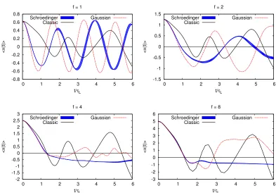
In Fig.1we compare the time dependence of the expectation valuexˆ(t)of thexcoordinate, obtained from the classical equations of motion, from the Gaussian state approximation, and from the numerical solution of the Schrödinger equation. From the topmost plot on the left to the lowest plot on the right we increase the initial expectation values ofxandycoordinates (factorf in (10)) as compared to the quantum dispersions which are fixed for all f. We thus move from the quantum regime at small f to the classical regime at large f. We note that as f becomes larger, the classical solution is rescaled asx(t)→ f x(f t) - that is, the classical dynamics becomes faster, and the corresponding classical Lyapunov exponentλcL becomes f times larger. To make the comparison of different
real-time evolution methods independent of this trivial classical scaling of the Lyapunov exponent, we express the physical timetin units of the classical Lyapunov timeτcL≡λcL−1.
One can see that when the expectation valuesx,yare not very large compared to the corre-sponding quantum dispersions (f = 1, f =2), the difference between the classical solution and the
solution of the Schrödinger equation is rather large even at early evolution times. The Gaussian state approximation is much closer to the full quantum evolution forλcLt1. For f =1, the Gaussian state
approximation also captures the period and the amplitude of the oscillations ofxˆ(t)rather well. At larger f =4 and f =8 we see how the classical dynamics becomes more and more exact at early
timesλcLt1, and the numerical accuracy of the Gaussian state approximation extends even further toλcLt2. In contrast, the late-time dynamics is captured less and less precisely as the initial expec-tation valuesx,ybecome larger. In particular, while at f =4 the Gaussian state approximation
describes rather well the suppression of oscillations ofxˆ(t)as compared to the classical dynamics, for the largest f =8 at late times both the classical dynamics and the Gaussian state approximation
to the full Schrödinger equation, the number of variables in the equations (6) and (9) grows only quadratically in the number of degrees of freedom.
Let us now compare the numerical solution of the equations (6) and (9) with the solution of the full Schrödinger equation. We consider the pure Gaussian state with initially nonzero expectation values ofxandyand the minimal quantum dispersion saturating the uncertainty relation:
x=0.625f, y=0.325f, xx=yy=pxpx=pypy=1/2,
px=py=xy=pxpy=pxx=pxy=pyy=pxx=0. (10) The variable f controls the dominance of the “classical” expectation valuesx andy over the quantum dispersions.
To solve the time-dependent Schrödinger equation, we replace the continuum coordinatesxandy
by a finite lattice with spacinga, with sites labelled by indicesi,j∈[−Ns+1,Ns]: xi=ai,yj=a j.
The potentialV(x, y)=x2y2/2 is turned into a periodic functionVi j=122Nsa π
2
sin2 πxi
2Nsa
sin2πyj
2Nsa
on this discrete periodic lattice.Vi jcoincides with the continuumV(x, y) for sufficiently smallxi,yj.
The operator ˆp2=−∂2
xis replaced by the sum of the usual lattice Laplacians−∆ii =2δi i−δi i+1− δi i−1 for bothxandycoordinates. We then perform the leapfrog-type evolution by multiplying the
wave functionψ(x, y)→ψi jby the unitary evolution operator
U(δt)=exp (iVδt/2) exp
ipˆ2
2 ∆t
exp (iVδt/2) (11)
with sufficiently small time step δt. In order to control discretization and finite-volume artifacts,
in addition to the solution with lattice spacinga, time step δtand lattice sizeNs we also consider
solutions with parameters{2a, δt,Ns},{a,2δt,Ns}and{a, δt,Ns/2}. We then estimate the discretization
and finite volume error of the expectation valuesOˆ(t)as the difference between their minimal and
maximal values over simulations with these four sets of parameters.
In Fig.1we compare the time dependence of the expectation valuexˆ(t)of thexcoordinate, obtained from the classical equations of motion, from the Gaussian state approximation, and from the numerical solution of the Schrödinger equation. From the topmost plot on the left to the lowest plot on the right we increase the initial expectation values ofxandycoordinates (factor fin (10)) as compared to the quantum dispersions which are fixed for all f. We thus move from the quantum regime at small f to the classical regime at large f. We note that as f becomes larger, the classical solution is rescaled asx(t) → f x(f t) - that is, the classical dynamics becomes faster, and the corresponding classical Lyapunov exponentλcLbecomes f times larger. To make the comparison of different
real-time evolution methods independent of this trivial classical scaling of the Lyapunov exponent, we express the physical timetin units of the classical Lyapunov timeτcL≡λcL−1.
One can see that when the expectation valuesx,yare not very large compared to the corre-sponding quantum dispersions (f =1, f =2), the difference between the classical solution and the
solution of the Schrödinger equation is rather large even at early evolution times. The Gaussian state approximation is much closer to the full quantum evolution forλcLt1. For f =1, the Gaussian state
approximation also captures the period and the amplitude of the oscillations ofxˆ(t)rather well. At larger f =4 and f =8 we see how the classical dynamics becomes more and more exact at early
timesλcLt 1, and the numerical accuracy of the Gaussian state approximation extends even further toλcLt2. In contrast, the late-time dynamics is captured less and less precisely as the initial expec-tation valuesx,ybecome larger. In particular, while at f =4 the Gaussian state approximation
describes rather well the suppression of oscillations ofxˆ(t)as compared to the classical dynamics, for the largest f =8 at late times both the classical dynamics and the Gaussian state approximation
are equally inaccurate.
-0.8 -0.6 -0.4 -0.2 0 0.2 0.4 0.6 0.8
0 1 2 3 4 5 6
<x(t)>
t/τ L
f = 1
Schroedinger Classic Gaussian -1.5 -1 -0.5 0 0.5 1 1.5
0 1 2 3 4 5 6
<x(t)>
t/τ L
f = 2
Schroedinger Classic Gaussian -2 -1.5 -1 -0.5 0 0.5 1 1.5 2 2.5 3
0 1 2 3 4 5 6
<x(t)>
t/τ L
f = 4
Schroedinger Classic Gaussian -3 -2 -1 0 1 2 3 4 5 6
0 1 2 3 4 5 6
<x(t)>
t/τ L
f = 8
Schroedinger
Classic Gaussian
Figure 1. Time dependence of the expectation valuesx(t), obtained from the classical equations of motion (solid black line), from the Gaussian state approximation (dotted red line) and from the numerical solution of the Schrödinger equation (blue strip with strip width estimating the finite-spacing and finite-volume artifacts). The initial state is the Gaussian state with center and dispersions given by (10), with f = 1 (top left), f =2 (top right),f =4 (bottom left) and f =8 (bottom right). The timetis in units of the inverse classical Lyapunov time
τcL≡λcL−1∼ f−1.
Finally, an important methodological question is how to control the validity of the Gaussian state approximation without having the reference solution of the Schrödinger equation, which is practically unfeasible for sufficiently large number of degrees of freedom. One of the possible intuitive criteria
is the importance of terms which contain squares of quantum dispersions in the potential energy
V(x, y) =x2y2/2 = x2y2+x2y2+y2x2+4xyxy+2xy2+x2y2. We have found that the Gaussian state approximation starts being inaccurate when the last two summands in the above expression forV(x, y)become comparable with the kinetic energyp2
x/2+p2y/2.
This replaces the condition of large occupation numbers for the classical dynamics.
3 Gaussian state approximation for matrix quantum mechanics
In this Section, we apply the Gaussian state approximation to the matrix quantum mechanics with the Hamiltonian (1). To this end we decompose the matrix-valued canonical variables XiandPi in the
basis of generatorsTaofS U(N) Lie algebra, with Tr (TaTb)=δaband [Ta,Tb]=iCabcTc:Xi=XiaTa,
now average the Heisenberg equations of motion with the Hamiltonian (1) over the most general Gaussian state characterized by the expectation valuesXa
i =Xˆia,Pia(t)=Pˆaiand the dispersions
Xa
iXbj,XaiPbjandPaiPbjdefined as in (5). We obtain the following equations of motion:
∂tXia=Pai, ∂tXiaXbj=XiaPbj+XbjPai, ∂tPai =−CabcCcdeXbjXidXej−
−CabcCcdeXbjXidXej −CabcCcdeXbjXejXid−CabcCcdeXbjXidXej, (12)
∂tXiaPkf=PaiPkf −CabcCcdeXdiXejXbjXkf −
−CabcCcdeXbjXejXidXkf −CabcCcdeXbjXidXejXkf,
∂tPaiPkf=−CabcCcdeXdiXejXbjPkf −
−CabcCcdeXbjXejXidPkf −CabcCcdeXbjXdi XejPkf+({a,i} ↔ {f,k}).
To study how quantum effects influence the classically chaotic dynamics of the Hamiltonian (1),
we extend the definition of Lyapunov exponents to the quantum case by considering two solutions of the equations (12) for which the initial Gaussian states differ by a very small shift of the wave packet
centerXa
i →Xai+ia. For the chaotic system, the differenceδXiabetween the expectation valuesXiafor
these two solutions should first grow exponentially as|δXa
i| ∼ |ia|exp (λLt), whereλLis the leading
Lyapunov exponent, and then saturate at a typical scale set by the system size. It is also easy to see that this definition is equivalent to the “out-of-time-order” correlator
δXia=in|ei
a iPˆaiXˆb
j(t)e−i
a
iPˆai |in − in|Xˆ(t)|in=iin|Pˆa
i(0),Xˆbj(t)
|inia. (13)
Our simulations were performed withd = 9 compactified spatial dimensions (motivated by the
BFSS matrix model [14]) andS U(5) Lie algebra. The initial values of the coordinatesXa
i (t=0)
of the wave packet center were randomly drawn from the Gaussian distribution with dispersionσ2, the initial values of momentaPa
i(t=0) were set to zero. The quantum dispersions were set to the
valuesXa
iXbj = δabδi jσxx, PaiPbj = δabδi jσpp, XaiPbj = 0, σxx = (N(d−1))−1/3/2,
σpp =1/(4σxx) which minimize the expectation value of the Hamiltonian (1) in the space of pure
Gaussian states. We chooseiato be a random vector with|ai|=0.00001. We illustrate the time dependence of the distance|δXa
i|between two close solutions of the
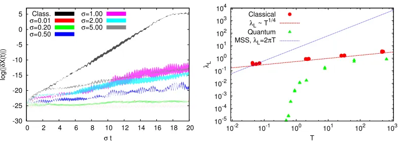
equa-tions (12) in the left plot on Fig.2. For comparison we also show the time dependence of|δXa i|for the
classical equations of motion. Since even the classical Lyapunov exponents depend on the scale ofXa i
variables asλcL∼σ, we useσt∼λcLtfor the time coordinate. The classical dynamics exhibits a clear exponential growth|δX(t)| ∼exp (λLt) with time, followed by the expectable saturation of Lyapunov
distance at late times for a bound system. For quantum dynamics the growth rate of the Lyapunov distance coincides with the classical one only at some initial period of time, which becomes larger as the dynamics becomes more classical at largerσ. Presumably, this initial period of time can be related
to the thermalization of our “artificial” initial state itself, which is then followed by the decay of small perturbations on top of the more universal thermalized state. At later times the leading Lyapunov exponentλLfor the quantum dynamics turn out to be several times smaller.
Let us now consider the temperature dependence of the quantum Lyapunov exponents obtained numerically from the correlator (13). In order to introduce temperature, we rely on the chaotic, “self-averaging” classical dynamics of the Hamiltonian (1) which implies the equivalence between canon-ical and micro-canoncanon-ical ensembles. At sufficiently high energies and temperatures we can use the
classical equation of state [15,16]
E=χT, χ=3
4
(d−1)N2−1−d(d−1) 2
now average the Heisenberg equations of motion with the Hamiltonian (1) over the most general Gaussian state characterized by the expectation valuesXa
i =Xˆia,Pia(t)=Pˆaiand the dispersions
Xa
iXbj,XiaPbjandPaiPbjdefined as in (5). We obtain the following equations of motion:
∂tXia=Pai, ∂tXiaXbj=XiaPbj+XbjPai, ∂tPai =−CabcCcdeXbjXdiXej−
−CabcCcdeXbjXidXej −CabcCcdeXbjXejXid−CabcCcdeXbjXdi Xej, (12)
∂tXaiPkf=PaiPkf −CabcCcdeXidXejXbjXkf −
−CabcCcdeXbjXejXidXkf −CabcCcdeXbjXidXejXkf,
∂tPaiPkf=−CabcCcdeXidXejXbjPkf −
−CabcCcdeXbjXejXidPkf −CabcCcdeXbjXdi XejPkf+({a,i} ↔ {f,k}).
To study how quantum effects influence the classically chaotic dynamics of the Hamiltonian (1),
we extend the definition of Lyapunov exponents to the quantum case by considering two solutions of the equations (12) for which the initial Gaussian states differ by a very small shift of the wave packet
centerXa
i →Xai+ia. For the chaotic system, the differenceδXiabetween the expectation valuesXiafor
these two solutions should first grow exponentially as|δXa
i| ∼ |ia|exp (λLt), whereλLis the leading
Lyapunov exponent, and then saturate at a typical scale set by the system size. It is also easy to see that this definition is equivalent to the “out-of-time-order” correlator
δXai =in|ei
a iPˆaiXˆb
j(t)e−i
a
iPˆai|in − in|Xˆ(t)|in=iin|Pˆa
i(0),Xˆbj(t)
|inia. (13)
Our simulations were performed withd = 9 compactified spatial dimensions (motivated by the
BFSS matrix model [14]) andS U(5) Lie algebra. The initial values of the coordinates Xa
i (t=0)
of the wave packet center were randomly drawn from the Gaussian distribution with dispersionσ2, the initial values of momentaPa
i(t=0) were set to zero. The quantum dispersions were set to the
valuesXa
iXbj = δabδi jσxx, PaiPbj = δabδi jσpp, XiaPbj = 0, σxx = (N(d−1))−1/3/2,
σpp =1/(4σxx) which minimize the expectation value of the Hamiltonian (1) in the space of pure
Gaussian states. We chooseiato be a random vector with|ia|=0.00001. We illustrate the time dependence of the distance|δXa
i|between two close solutions of the
equa-tions (12) in the left plot on Fig.2. For comparison we also show the time dependence of|δXa i|for the
classical equations of motion. Since even the classical Lyapunov exponents depend on the scale ofXa i
variables asλcL∼σ, we useσt∼λcLtfor the time coordinate. The classical dynamics exhibits a clear exponential growth|δX(t)| ∼exp (λLt) with time, followed by the expectable saturation of Lyapunov
distance at late times for a bound system. For quantum dynamics the growth rate of the Lyapunov distance coincides with the classical one only at some initial period of time, which becomes larger as the dynamics becomes more classical at largerσ. Presumably, this initial period of time can be related
to the thermalization of our “artificial” initial state itself, which is then followed by the decay of small perturbations on top of the more universal thermalized state. At later times the leading Lyapunov exponentλLfor the quantum dynamics turn out to be several times smaller.
Let us now consider the temperature dependence of the quantum Lyapunov exponents obtained numerically from the correlator (13). In order to introduce temperature, we rely on the chaotic, “self-averaging” classical dynamics of the Hamiltonian (1) which implies the equivalence between canon-ical and micro-canoncanon-ical ensembles. At sufficiently high energies and temperatures we can use the
classical equation of state [15,16]
E=χT, χ=3
4
(d−1)N2−1−d(d−1) 2 (14) -30 -25 -20 -15 -10 -5 0 5
0 2 4 6 8 10 12 14 16 18 20
log(|
δ
X(t)|)
σ t
Class. σ=0.01 σ=0.20 σ=0.50 σ=1.00 σ=2.00 σ=5.00 10-5 10-4 10-3 10-2 10-1 100 101 102 103 104
10-2 10-1 100 101 102 103
λL
T Classical
λL ~ T1/4 Quantum
MSS, λL=2πT
Figure 2.A comparison of Lyapunov instability of the matrix quantum mechanics with the Hamiltonian (1) in the classical and in the Gaussian state approximations. On the left: time dependence of the Lyapunov distance between two initially close solutions of the evolution equations. On the right: temperature dependence of the leading Lyapunov exponents for classical and quantum dynamics compared with the MSS bound. We change the classical dispersionσof the initial values ofXa
i coordinates and keep fixed the initial quantum dispersion. On the right plot, the equations of state (14) and (15) are used to express temperature in terms of energy.
to translate energyE into temperatureT. At low temperatures, this equation of state changes due to quantum effects. In particular, in the limit of zero temperature the energy approaches some finite
valueE0 of the ground-state energy [17]. To be consistent with the Gaussian state approximation, the ground state energy should be defined by minimizing the Hamiltonian (1) over all pure Gaus-sian states, which yieldsE0 = 38d(d−1)1/3N1/3
N2−1. In order to interpolate between the low-temperature asymptoticsE → E0 (atT → 0) and the classical high-temperature equation of state (14), we use a phenomenological formula
E=E0/tanh
E0
χT
, E0 =3
8d(d−1)1/3N1/3
N2−1. (15)
Since the first-principle equation of state of [17] would be anyway inconsistent with the Gaussian state approximation, we prefer to use the artifical equation of state (15). The most important conclusions of this work should not dramatically depend on moderate changes in the equation of state.
Temperature dependence of quantum Lyapunov exponents is illustrated on the right plot on Fig.2. For comparison, we also show the temperature dependence of the classical Lyapunov exponents, which is well described by the formulaλL =
0.292−0.42/N2T1/4 [16], with the temperatureT defined from (14). We see that quantum corrections tend to decrease the Lyapunov exponents at intermediate temperatures. Moreover, at some “critical” temperatureTc ≈0.6 the leading Lyapunov
exponent seem to vanish. Interestingly, first-principle Monte-Carlo simulations indicate that in the large-Nlimit the matrix quantum mechanics (1) has a finite-temperature confinement-deconfinement phase transition at roughly the same temperatureT
c ≈ 0.9 [17]. This has to be contrasted with the
supersymmetric BFSS model, which is not confining all the way down to the strong-coupling regime atT = 0. By analogy with N = 4 super-Yang-Mills in D = 3 +1, we expect the MSS bound λL<2πT [18] to be saturated in this regime. On the other hand, in the confinement phase of the
non-supersymmetric Hamiltonian (1), it is natural to expect that Lyapunov exponents are 1/N-suppressed,
corrections at low temperatures and probably the confinement-deconfinement transition prevent the violation of MSS bound, which for classical Lyapunov exponents happens at the temperatureT = 0.292−0.42/N2
2π 4/3
=0.015 which is much lower thanTc.
4 Discussion and outlook
In these Proceedings we have outlined the Gaussian state approximation for the real-time dynam-ics of many-body systems, used previously in the quantum chemistry context [8], and demonstrated on a simple example that it is capable of reproducing the essential features of quantum dynamics which are absent for the classical equations of motion. We applied this approximation to study the real-time dynamics of the matrix quantum mechanics, and found that quantum corrections tend to decrease the leading Lyapunov exponentλLextracted from the simplest out-of-time-order correlator
in|Pˆa
i (0),Xˆia(t)
|in. We have shown that quantum corrections seem to be large enough to ensure the validity of the MSS boundλL < 2πT at sufficiently low temperatures. Of course, we can make
this statement only up to the unquantified systematic error of the Gaussian state approximation, which becomes quantitatively worse at low temperatures (see Fig.1for illustration). In particular, it would be interesting to understand in more details whether the vanishing of quantum Lyapunov exponents below some finite temperature is a signature of the finite-temperature phase transition found in [17], or rather an artifact of the Gaussian state approximation.
The generalization of the Gaussian state approximation to Yang-Mills theory should not meet significant conceptual difficulties. The resulting algorithm would require the number of Flops
propor-tional to the square of the number of (spatial) lattice sites, which should allow for simulations on not very large lattices with modest computational resources.
References
[1] A. Kurkela, G.D. Moore, JHEP1112, 044 (2011),1107.5050
[2] A. Kurkela, Y. Zhu, Phys. Rev. Lett.115, 182301 (2015),1506.06647
[3] H. Nastase,The RHIC fireball as a dual black hole(2005),hep-th/0501068
[4] J. Schmiedmayer, J. Berges, Science341, 1188 (2013)
[5] K. Dusling, T. Epelbaum, F. Gelis, R. Venugopalan, Nucl. Phys. A850, 69 (2011),1009.4363
[6] T. Kunihiro, B. Müller, A. Ohnishi, A. Schäfer, Prog. Theor. Phys.121, 555 (2009),0809.4831
[7] P. Arnold, G.D. Moore, L.G. Yaffe, JHEP0301, 030 (2003),hep-ph/0209353
[8] J. Broeckhove, L. Lathouwers, P. van Leuven, J. Mol. Struct.: THEOCHEM199, 245 (1989) [9] G.K. Savvidy, Nucl. Phys. B246, 302 (1984)
[10] C.T. Asplund, D. Berenstein, D. Trancanelli, Phys. Rev. Lett.107, 171602 (2011),1104.5469
[11] C.T. Asplund, D. Berenstein, E. Dzienkowski, Phys. Rev. D87, 084044 (2013),1211.3425
[12] S. Aoki, M. Hanada, N. Iizuka, JHEP1507, 029 (2015),1503.05562
[13] E. Witten, Nucl. Phys. B460, 335 (1996),hep-th/9510135
[14] T. Banks, W. Fischler, S.H. Shenker, L. Susskind, Phys. Rev. D 55, 5112 (1997),
hep-th/9610043
[15] N. Kawahara, J. Nishimura, S. Takeuchi, JHEP0712, 103 (2012),0710.2188
[16] G. Gur-Ari, M. Hanada, S.H. Shenker, JHEP1602, 091 (2016),1512.00019
[17] N. Kawahara, J. Nishimura, S. Takeuchi, JHEP0710, 097 (2007),0706.3517