Scholarship@Western
Scholarship@Western
Electronic Thesis and Dissertation Repository
8-24-2018 11:00 AM
High Performance Sparse Multivariate Polynomials: Fundamental
High Performance Sparse Multivariate Polynomials: Fundamental
Data Structures and Algorithms
Data Structures and Algorithms
Alex BrandtThe University of Western Ontario
Supervisor
Moreno Maza, Marc
The University of Western Ontario
Graduate Program in Computer Science
A thesis submitted in partial fulfillment of the requirements for the degree in Master of Science © Alex Brandt 2018
Follow this and additional works at: https://ir.lib.uwo.ca/etd
Part of the Algebra Commons, Numerical Analysis and Scientific Computing Commons, and the
Theory and Algorithms Commons
Recommended Citation Recommended Citation
Brandt, Alex, "High Performance Sparse Multivariate Polynomials: Fundamental Data Structures and Algorithms" (2018). Electronic Thesis and Dissertation Repository. 5593.
https://ir.lib.uwo.ca/etd/5593
This Dissertation/Thesis is brought to you for free and open access by Scholarship@Western. It has been accepted for inclusion in Electronic Thesis and Dissertation Repository by an authorized administrator of
Abstract
Polynomials may be represented sparsely in an effort to conserve memory usage and pro-vide a succinct and natural representation. Moreover, polynomials which are themselves sparse – have very few non-zero terms – will have wasted memory and computation time if represented, and operated on, densely. This waste is exacerbated as the number of variables increases. We provide practical implementations of sparse multivariate data structures focused on data locality and cache complexity.
We look to develop high-performance algorithms and implementations of fundamen-tal polynomial operations, using these sparse data structures, such as arithmetic (ad-dition, subtraction, multiplication, and division) and interpolation. We revisit a sparse arithmetic scheme introduced by Johnson in 1974, adapting and optimizing these algo-rithms for modern computer architectures, with our implementations over the integers and rational numbers vastly outperforming the current wide-spread implementations. We develop a new algorithm for sparse pseudo-division based on the sparse polynomial division algorithm, with very encouraging results. Polynomial interpolation is explored through univariate, dense multivariate, and sparse multivariate methods. Arithmetic and interpolation together form a solid high-performance foundation from which many higher-level and more interesting algorithms can be built.
Keywords: Sparse Polynomials, Polynomial Arithmetic, Polynomial Interpolation, Data Structures, High-Performance, Polynomial Multiplication, Polynomial Division, Pseudo-Division
Abstract i
List of Tables iv
List of Figures v
List of Algorithms vi
1 Introduction 1
1.1 Existing Computer Algebra Systems and Software . . . 2
1.2 Reinventing the Sparse Polynomial Wheel? . . . 3
1.3 Contributions . . . 4
2 Background 6 2.1 Memory, Cache, and Locality . . . 6
2.1.1 Cache Performance and Cache Complexity . . . 7
2.2 Algebra . . . 9
2.2.1 The Many Flavours of Rings . . . 9
2.2.2 Polynomials: Rings, Definitions, and Notations . . . 11
2.2.3 Arithmetic in a Polynomial Ring . . . 14
Pseudo-division . . . 16
2.2.4 Gr¨obner Bases, Ideals, and Reduction . . . 17
2.2.5 Algebraic Geometry . . . 20
2.2.6 (Numerical) Linear Algebra . . . 21
2.3 Representing Polynomials . . . 22
2.4 Working with Sparse Polynomials . . . 24
2.5 Interpolation & Curve Fitting . . . 27
2.5.1 Lagrange Interpolation . . . 30
2.5.2 Newton Interpolation . . . 31
2.5.3 Curve Fitting and Linear Least Squares . . . 32
2.6 Symbols and Notation . . . 33
3 Memory-Conscious Polynomial Representations 35 3.1 Coefficients, Monomials, and Exponent Packing . . . 36
3.2 Linked Lists . . . 38
3.3 Alternating Arrays . . . 38
3.4 Recursive Arrays . . . 42
4 Polynomial Arithmetic 45 4.1 In-place Addition and Subtraction . . . 45
4.2 Multiplication . . . 47
4.2.1 Implementation . . . 51
Heap Optimizations . . . 52
4.2.2 Experimentation . . . 54
4.3 Division . . . 59
4.3.1 Implementation . . . 63
4.3.2 Experimentation . . . 64
4.4 Pseudo-Division . . . 66
4.4.1 Implementation . . . 70
4.4.2 Experimentation . . . 72
4.5 Normal Form and Multi-Divisor Pseudo-Division . . . 75
5 Symbolic and Numeric Polynomial Interpolation 76 5.1 Univariate Polynomial Interpolation . . . 77
5.2 Dense Multivariate Interpolation . . . 81
5.2.1 Implementing Early Termination for Multivariate Interpolation . . 83
5.2.2 The Difficulties of Multivariate Interpolation . . . 85
5.2.3 Rational Function Interpolation . . . 88
5.3 Sparse Multivariate Interpolation . . . 90
5.3.1 Probabilistic Method . . . 90
5.3.2 Deterministic Method . . . 94
5.3.3 Experimentation . . . 97
5.4 Numerical Interpolation (& Curve Fitting) . . . 99
6 Conclusions and Future Work 101
Bibliography 103
Curriculum Vitae 108
4.1 Comparing heap implementations with and without chaining . . . 56 4.2 Comparing pseudo-division on triangular decompositions . . . 75
List of Figures
2.1 Array representation of a dense univariate polynomial . . . 22
2.2 Array representation of a dense recursive multivariate polynomial . . . . 24
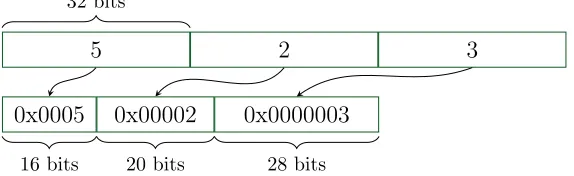
3.1 A 3-variable exponent vector packed into a single machine word. . . 37
3.2 A polynomial encoded as a linked list . . . 38
3.3 A polynomial encoded as an alternating array . . . 39
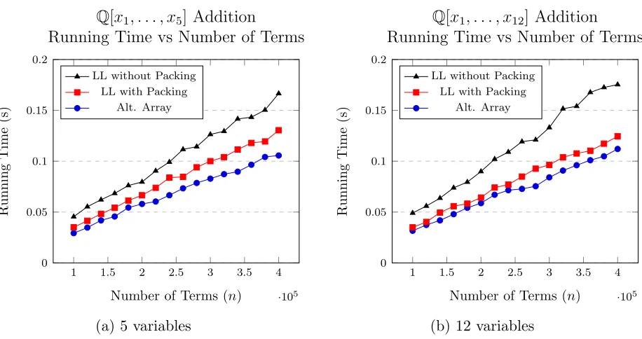
3.4 Comparing linked list and alternating array implementations of polynomial addition . . . 40
3.5 Comparing cache misses in polynomial addition . . . 41
3.6 Array representation of a dense recursive multivariate polynomial . . . . 42
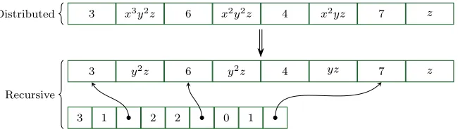
3.7 An alternating array and recursive array polynomial representation . . . 43
4.1 Alternating array representation showing GMP trees . . . 46
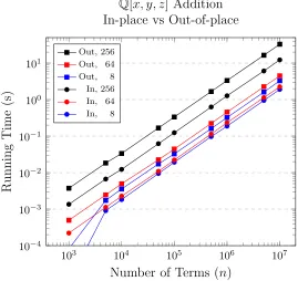
4.2 Comparing in-place and out-of-place polynomial addition . . . 47
4.3 An example heap of integers . . . 48
4.4 A chained heap of product terms . . . 55
4.5 Comparing multiplication of integer polynomials . . . 57
4.6 Comparing multiplication of rational number polynomials . . . 58
4.7 Comparing cache misses in polynomial multiplication . . . 58
4.8 Comparing division of integer polynomials . . . 65
4.9 Comparing division of rational number polynomials . . . 65
4.10 A recursive polynomial representation for a pseudo-quotient . . . 71
4.11 Comparing pseudo-division of integer polynomials . . . 73
4.12 Comparing pseudo-division of rational number polynomials . . . 73
4.13 Comparing naive and heap-based pseudo-division . . . 74
5.1 Comparing univariate interpolation implementations . . . 80
5.2 A collection of points satisfying condition GC . . . 87 5.3 Comparing probabilistic and deterministic sparse interpolation algorithms 98
2.1 polynomialDivision . . . 16
2.2 na¨ıvePseudoDivision . . . 17
2.3 addPolynomials . . . 26
2.4 multiplyPolynomials . . . 28
4.1 heapMultiplyPolynomials. . . 49
4.2 dividePolynomials. . . 59
4.3 heapDividePolynomials . . . 61
4.4 pseudoDividePolynomials . . . 67
4.5 heapPseudoDividePolynomials . . . 69
5.1 LagrangeInterpolation . . . 79
5.2 multiplyByBinomial InPlace . . . 80
5.3 denseInterpolation Driver . . . 84
5.4 sparseInterpolation StageI . . . 93
5.5 sparseInterpolation . . . 93
5.6 sparseInterpolation StageI Deterministic . . . 96
5.7 sparseInterpolation Deterministic . . . 96
Chapter 1
Introduction
In the world of computer algebra and scientific computing, high-performance is paramount. Due to the exact nature of symbolic computations (in fact that is one of the defining characteristics of computer algebra) it is possible to be far more expressive than in nu-merical methods, leading to more complicated mathematical formulas and theories. But as these formulas, problems, and data sets grow large, the intermediate expressions which arise during the process of solving these problems grow even larger. Thisexpression swell
is one reason why computer algebra has historically been seen as slow and impractical. Compared to that of numerical analysis, where floating point numbers occupy a fixed amount of space regardless of their value, symbolic computation uses arbitrary precision, allowing numbers to grow and grow. Hence, careful implementation is needed to avoid such drastic slow downs and make symbolic computation able to be practical and useful in solving mathematical and scientific problems.
One such problem we are concerned with is polynomial system solving. Of course, this is an important problem with applications in every scientific discipline. Algorithms for solving these systems typically rely on somecore operation after some algebraic tricks attempt to reduce the system’s complexity. This core operation could be based on Gr¨obner bases or triangular decompositions. We are motivated by the efforts to ob-tain an efficient and open source implementation of triangular decompositions using the theory of regular chains [4]. Such algorithms [18] have already been integrated into the computer algebra system Mapleas part of theRegularChainslibrary [53]. However,
we believe that we can do better.
The Basic Polynomial Algebra Subprograms (BPAS) library [2] is an open-source li-brary for high performance polynomial operations, such as arithmetic, real root isolation, and polynomial system solving. It is mainly written in Cfor performance, with a C++ wrapper interface for portability, object-oriented programming, and end-user usability. Moreover, it makes use of the Cilk extension [52] for parallelization and improved
per-formance on multi-core processors. It is within this library that we include our sparse polynomial data structures and high-performance implementations for fundamental
erations in support of triangular decompositions and regular chains. The algorithms and implementations presented here are published within the BPAS library.
In particular, we provide highly optimized implementations of sparse multivariate polynomials over the integers and rational numbers. This includes memory-efficient data structures, finely-tuned arithmetic (addition, multiplication, division, pseudo-division), as well as interpolation. The operations of arithmetic and interpolation are absolutely fundamental to any algorithm dealing with polynomials. The fundamental nature of arithmetic should be obvious. Of course one cannot hope to implement any form of performance mathematical algorithm without the basic arithmetic also being high-performance. From this standpoint we look to build from the ground up, providing the fastest arithmetic possible so that it can be put to use in higher level algorithms.
The fundamental nature of interpolation is less obvious without considering evaluation-interpolation schemes as part ofmodular methods. To combat the expression swell char-acteristic of symbolic computations, the approach of modular methods is to solve a large number of simplified problems where the values for the variables are carefully chosen (evaluation) and, using the results of each of these simplified problems, a solution to the original problem is reconstructed (interpolation) [75]. These methods are used extensively throughout computer algebra [31, Chapter 5].
In either case, our optimized, high-performance implementations of sparse polyno-mial data structures and algorithms provide a solid foundation from which we can build upon to better the algorithms and implementations available in computer algebra and scientific computing.
1.1
Existing Computer Algebra Systems and
Soft-ware
The ALTRAN system for multivariate rational functions [37], developed in the late
sixties at Bell Labs, was one of the first computer algebra systems. It too made use of sparse polynomials in its computations for effective memory usage and performance.
Since that time, many computer algebra systems, proprietary and open source, have been developed. The most notable of which is likely Maple. It began in 1982, and since then has found its way into scientific computing, industrial applications, and many university classrooms. Vast amounts of research has gone into developing Maple, and,
as of 2011, has become a leader in performance because of this [56–59].
This is not to outshine the many other computer algebra systems which are also leaders in their own right. To name a few, there are Mathematica [72], Trip [30], Magma [14], Singular [65], CoCoA [34], and Symbolic Math Toolbox of MATLAB.
1.2. Reinventing the Sparse Polynomial Wheel? 3
common libraries which are focused on number theory, but provide powerful univariate symbolic computation nonetheless areNTL[71] andFLINT[38]. SymPy [55], a Python
library for symbolic computations is actively being developed and excels in usability, a property for which Python is well known.
Maple andTrip are both known to use sparse polynomials in their computations.
Interestingly, these are the overwhelmingly highest performing implementations [56–58]. This goes to show, that although recent decades were spent in the computer algebra community developing dense algorithms for polynomial arithmetic [12, 46, 69], all is not lost in the world of sparse polynomials.
With the work presented here on optimized sparse polynomials, we hope to make the BPAS library a leader in performance as well as availability through an open-source codebase.
1.2
Reinventing the Sparse Polynomial Wheel?
Several decades ago, algorithms and implementations of sparse polynomials was a major topic of research. The seminal articles on sparse polynomial arithmetic by Johnson [42], and sparse polynomial interpolation by Zippel [76] are two excellent examples from the seventies. The ALTRAN system of the late sixties [37], made exclusive use of sparse
representations for its multivariate rational functions.
Alas, these algorithms and technologies are now nearly 50 years old. In terms of computing technology, they may as well be millennia old. The motivation for sparse algorithms and representations at the time was a result of limited computing resources. The computing memory available then was not even comparable to modern computers. As late as 1980, computer scientists were still using memory chips of a mere 64 megabytes [39, Section 1.4]. Today, 64 gigabytes is common even in consumer-level computers, let alone high performance server units. As a result of this limited memory, algorithms had been developed to minimize the amount of memory used.
On modern computer architectures, the amount of memory used is much less im-portant. Rather, we are far more concerned with how memory is used. This is due to
the memory wall – “[the] point system performance is totally determined by memory
speed; making the processor faster won’t affect the wall-clock time to complete an ap-plication.”[73, p. 21]. The authors of [73] suggest a possible solution: make caches work better, having cache hits occur as frequently as possible. In their point of view, this was an architectural problem for computers.
memory to avoid latent memory accesses. Computer scientists and programmers need to be aware of memory usage and memory access patterns in order to minimize the impact of waiting for latent memory. The formalization of cache complexity [28] is one step toward this. Apart from a usual time complexity analysis of an algorithm, which is only concerned with number of computational steps, cache complexity measures how an algorithm makes use of memory, and therefore also an important indicator of performance given the current processor-memory gap [39] (see Section 2.1).
It is with this mindset that we look to implement sparse polynomial data structures and algorithms. We are concerned with performance on modern day architectures, by handling memory effectively, optimizing for cache complexity, and minimizing the impact of the processor-memory gap. Hence, while sparse polynomials have been around for many years, they had been developed using wildly different frames of reference and motivating factors than are no longer applicable.
1.3
Contributions
Throughout all of the work we present here, we are looking to give a fresh implementation of sparse polynomial algorithms for modern day architectures. We look to answer the following questions:
(1) How can the limitations of modern architecture be handled in practical implemen-tations of existing algorithms?
(2) How can we adapt the ideas of classical sparse algorithms to new operations? (3) How worthwhile is the effort to more finely implement (and make publicly available)
existing high-performance algorithms?
We believe these questions have been answered thoroughly over the course of this thesis.
As mentioned in the previous section, our implementations are concerned with ef-ficient memory management, memory traversal, and thus cache complexity. It is with this perspective that we approach our implementations. From Johnson’s sparse addition, multiplication and division, to Zippel’s sparse interpolation, we make great efforts to optimize memory usage through data structures and practical implementations with low cache complexity.
Using the ideas of Johnson, and the ideas we discovered through the process of implementing the basic polynomial arithmetic functions (addition, subtraction, multipli-cation, division), we propose a new algorithm for sparse pseudo-division. Modeling this algorithm off sparse polynomial division, we implement it effectively, with very promising results.
1.3. Contributions 5
implemented in an optimal manner. We are not the first to do so. In [56–59] Monagan and Pearce have also realized Johnson’s decades old algorithms on modern computers. Their implementation is exclusive to the proprietary software within Maple. However,
with some of their optimization techniques in publication, we analyze and adjust their optimizations while adding some of our own, in order to fine-tune performance and achieve 50-100% speedup in comparison to their implementation. The story is similar for interpolation where we have developed an implementation of Lagrange interpolation which also out-performs that available inMaple. This time, however, we are an order of
magnitude faster. Hence, it is indeed worthwhile to spend effort on fine-tuning existing algorithms, as the resulting speed up can be dramatic with careful implementation.
To completely and accurately answer these questions, we organize this thesis as fol-lows. Chapter 2 begins the thesis by provided a background of knowledge for the many concepts touched on throughout later chapters. Since the subject matter of this thesis in-cludes an interesting overlap of algorithms, practical implementations, and mathematical concepts, we provide the necessary details that either a computer scientist or a mathe-matician may need to appreciate the other side. This includes: computer memory archi-tectures and cache complexity; rings, integral domains, fields, polynomials, and Gr¨obner bases; a short review of existing sparse polynomial techniques; and, a formalization of interpolation and some classical methods.
Chapter 3 discusses the effective encoding and data structures required to repre-sent polynomials as effectively as possible on modern computers, while making them favourable for use in our algorithms. These fundamental algorithms are presented in Chapter 4. There, algorithms, implementations, optimization techniques, and exper-imentation is presented for polynomial addition, subtraction, multiplication, division, and pseudo-division.
Background
Computer algebra lies in an interesting overlap of computer science and mathematics, drawing on both areas to fulfill its needs. In this background section, we introduce topics necessary to discuss our algorithms and implementations of polynomials. This includes some mathematics which computer scientists may be unfamiliar with, as well as some computer science aspects mathematicians may be unfamiliar with.
We discuss computer organization and memory hierarchy (Section 2.1); the under-standing of memory is important for developing high-performance algorithms. We also discuss some fundamentals of algebra, such as rings and operations defined within them (Section 2.2). A more specific presentation of polynomials, their representations, and a short history of sparse polynomial algorithms is given in Sections 2.3 and 2.4. Lastly, we present the problems of interpolation and curve fitting as well as some their classical solutions (Section 2.5).
2.1
Memory, Cache, and Locality
The structure of computer memory is no longer just important to the computer architect. Any programmer should have at least a basic understanding of its workings in order to produce good quality code. The reason for this is (somewhat) recent advancements in technology. The speed of processors has eclipsed the speed of computer memory many times over [39, Figure 5.2]. This difference is called the processor-memory gap. Decades ago, the speed of processors and memory were comparable, but the amount of memory available was limited. The problem now is different. There is (relatively) ample amounts of memory but it is slow to access compared to the speed of the processor. Because of this, programmers must change the way that they program in order make full use of the hardware.
Without considering a computer’s memory architecture, a program will almost surely
2.1. Memory, Cache, and Locality 7
underutilise the processor, as it sits idle waiting for latent memory accesses. Computer architects have attempted to close the processor-memory gap by creating a memory hierarchy. That is, a hierarchy of different forms of memory with increasing speeds but decreasing size. This forms the classical memory pyramid, with L1 cache at the top, followed by L2 and L3 cache, dynamic main memory, and finally hard disks (virtual memory).
L1 cache is the fastest memory, but has the smallest capacity. Ideally, for the best performance, we would want all of our data stored in L1 cache for the duration a program or algorithm. But due to the small capacity of L1 cache this is generally impossible. Not all hope is lost, as one can make use of theprinciple of locality — programs tend to reuse data and instructions which they have used recently [39, Section 1.9]. Therefore we have
data locality and instruction locality; the differentiation between the two is sometimes useful.
The principle of locality was put into the design of the memory hierarchy. Therefore, the choice of which data is stored in cache over main memory is a result of simply caching the data which has been most recently used. In practice, locality is implemented in a cache structure byevicting the least recently used item once a cache has reached capacity and attempts to load an additional item. Programmers must make use of this fact, by programming in such a way that exploits locality, and does not destroy it. There are two types of locality and we must be concerned with both. Temporal locality, which says that the most recently accessed items will likely be accessed again soon, and spatial locality, which says that the items adjacent to the most recently accessed items are also likely to be accessed soon. It is important to use these facts in programming. If an algorithm (or data structure) is implemented effectively, memory access time is greatly reduced by exploiting caching and locality [39, Chapter 5]. This is evident in our discussion of polynomial data structures (in particular, see Figures 3.4 and 3.5).
2.1.1
Cache Performance and Cache Complexity
Patterson and Hennessy [39, Section 5.7] are keen to highlight that a good cache ar-chitecture does necessarily give rise to good algorithms. Different algorithms use cache differently and the performance of one algorithm on one memory architecture does not imply the performance of another algorithm. Cache performance is a tricky thing to measure.
and how many layers away it is stored from the top-most cache. It could be in L2 cache, where the penalty is relatively small, or it could be stored in a page of virtual memory, which is much more costly. See [39, Appendix C] for details.
To avoid these architecture-dependent details of memory hierarchies and miss penal-ties, anidealized cache model [28] has been formulated. This model assumes a single cache with a single backing, arbitrarily large, main memory. In this model, the cache is broken incache lines, that is, the smallest unit of data that can move in and out of cache. One cache line always consists of sequential memory addresses. It is assumed that the cache can fitZ memory words and each line holdsLwords of that memory. Therefore, a cache has Z/L lines. Note a memory word is a fixed constant for a particular architecture, usually 4 or 8 bytes. This constant factor is therefore usually ignored, particularly in asymptotic analysis.
Using this model, it is possible not only to derive the normal time complexity of an algorithm, but alsocache complexity. Cache complexity is a way to measure and charac-terize and algorithm’s performance with respect to cache misses. It is paramecharac-terized by input size (n),Z, and L. It is also common to ignoreZ and Lin the analysis as they can be be implied by context, or could become simple constants in the complexity analysis which get removed by asymptotics (big-Oh notation).
Just as with time complexity, one wishes to minimize cache complexity in order to improve the theoretical (and indeed practical) performance of an algorithm. We have explained how caches work in reality, maintaining the most recently used items in cache. The ideal cache model works very similarly, but chooses to evict items which are next referenced furthest in the future, with items which are never referenced again being considered as the furthest possible in the future.
By this model, cache complexity can be reduced by exploiting locality as much as possible. The better locality that a program possesses, the better its cache performance. It is rather simple in that regard. But other aspects also affect cache performance. The size of data items plays an important role. Since the cache has a limited size (Z), if the individual data items being accessed require fewer bytes to store, than this will also improve cache complexity without altering locality. So, in summary, the two basic ways to improve cache complexity are:
(1) Exploit (data) locality to ensure memory is accessed sequentially or in an adjacent manner, and
(2) Reduce the amount of memory required for each data item so that more items can fit in cache at once. 1
It is clear that, given the processor-memory gap, practical implementations of any algorithms must be aware of cache performance and cache complexity. Naturally, our
1The same idea can technically be used for instructions as well, but they generally have fixed sizes
2.2. Algebra 9
algorithms are conscious of their memory usage and data locality in order to achieve high performance. The implementations details of these are explained in Sections 4.2.1, 4.3.1, 4.4.1, and 5.1.
For more details on computer architecture, memory, cache, and performance, Patter-son and Hennessy’sComputer Architecture provides plenty [39, Chapter 5 and Appendix C]. For a more detailed description of the ideal cache model and cache complexity, [28] and [66] are the defining works.
2.2
Algebra
This section is intended to introduce those unfamiliar with the mathematical technicali-ties of algebra, such as the average computer scientist, to a simple selection of concepts needed for our discussion of polynomial arithmetic and interpolation. This includes, rings, integrals domains, fields, the specifics of polynomials, and polynomials as rings. The appendix of Modern Computer Algebra [31] provides a useful overview and addi-tional details of all of these concepts. Here, we present only the ones necessary for our purposes.
2.2.1
The Many Flavours of Rings
A commutative ring (with identity) is a set R endowed with two binary operations, denoted + and ×. These operations need not be the usual addition and multiplication, but they must satisfy the following conditions:
(1) R is a commutative group under + with identity 0, (i) Associative: ∀a, b, c∈R, (a+b) +c=a+ (b+c), (ii) Identity: ∃0∈R ∀a∈R, a+ 0 =a,
(iii) Inverse: ∀a∈R ∃a−1 ∈R, a+a−1 = 0, and
(iv) Commutative: ∀a, b∈R, a+b=b+a; (2) × is associative and commutative;
(3) R has identity 1 for×; and
(4) × is distributive over +, ∀a, b, c∈R a×(b+c) = (a×b) + (a×c), and (b+c)×a= (b×a) + (c×a).
We assume that all rings are commutative and with a multiplicative identity unless explicitly stated. Such commutative rings are still quite general. Rings can be extended in many ways to obtain different specializations (“flavours”) with different properties.
Anintegral domain,D, (sometimes simplydomain) is a ring with the added property:
A zero divisor is an non-zero elementa∈Rwhere, for someb 6= 0∈R, we havea×b = 0. Thus, integral domains are suitable for looking at divisibility and exact division, without needing to worry2 about zero divisors. Aunit (orinvertible element) is an elementa ∈R
with a multiplicative inverse. That is, there existsb ∈R such that we have ab= 1.
Extending divisibility slightly with the notion of a greatest common divisor (GCD) then we get aGCD domain — an integral domain where any two elements have a GCD between them. IfR is a commutative ring with a multiplicative identity and if a, b, dare elements of R, we say that d is a common divisor of a and b if d divides both a and b; furthermore, we say thatdis agreatest common divisor ofaandb if any common divisor of a and b divides d as well.
The notion of a GCD domain is commonly used in computer algebra but it is rarely discussed in algebra textbooks, where the related (but not equivalent) concept is that of
a unique factorization domain (UFD). An integral domain U is a UFD whenever every
non-zero element of U writes as a product of irreducible elements, this factorization being unique up to the ordering of those irreducible elements and up to an invertible factor; for more details seehttps://en.wikipedia.org/wiki/Unique_factorization_ domain. Clearly, any two non-zero elements of a UFD have a GCD but the existence of an algorithm for computing such a GCD requires additional properties.
A fundamental example of UFDs where GCDs can be effectively computed are Eu-clidean domains. An integral domain D is an Euclidean domain whenever there exists a function| · |mapping every non-zero element of Dto a non-negative integer such that for alla, b∈D, withb 6= 0, there exists (q, r)∈D×Dsuch that we havea =qb+rand either
r= 0 or |r|<|b|holds; for a such pair (q, r) the elementsq andr are calledquotient and
remainder in the Euclidean division of a by b. The pair (q, r) is not necessarily unique (for instance in the case of the ring Z of the integer numbers) and additional properties may be required to make it unique (such as r≥0 in the case ofZ).
Afield,K, is an integral domain in which every non-zero element is a unit. This is a powerful property and it means that every element is divisible by every non-zero element inK. Equivalently, all divisions result in a 0 remainder.
A fundamental example of field construction is the field of fractions of an integral domain. This is a natural adaptation of the construction of the fieldQof rational numbers from the ring Z of integer numbers, to the case of an arbitrary integral domain D. For details, see https://en.wikipedia.org/wiki/Field_of_fractions.
All of these types of rings build upon the previous. Indeed, they form a strict class inclusion:
ring ⊃ integral domain ⊃ GCD domain ⊃ UFD ⊃ Euclidean domain⊃ field
2Indeed, ifRis an integral domain anda, b, q, q0 are elements ofRsuch thatb6= 0 anda=b q=b q0
2.2. Algebra 11
This inclusion is useful when we wish to speak generically about one type of ring. It then always applies to every subset of that type. This is evident beginning with polynomial rings.
2.2.2
Polynomials: Rings, Definitions, and Notations
A polynomial, as most know it, is a mathematical function in some variables, which is a linear combination of multiplicative combinations of those variables. For example,
p(x, y) = 5x3y2+ 3xy+ 4x+ 1. The multiplicative combinations are the sub-expressions
x3y2, xy, x, and 1 =x0y0. But, polynomials are far more sophisticated than that.
From the previous example, you can see there are essentially two parts which make up eachterm of a polynomial, the numerical coefficient and the multiplicative combination of the variables. This multiplicative combination is called a monomial. We say that the coefficients belong to some ring, R, and that the polynomial is formed over that base ring.
Polynomials themselves form rings, as one can add and multiply polynomials to-gether (see Section 2.2.3). Hence, we say polynomials over R to mean a ring of polyno-mials whose coefficients belong toR. However, we must also distinguish between different classes of polynomials over the same base ring. This is done by specifying the variables
(indeterminates) of the polynomials. Hence, our example polynomial p(x, y) would be a polynomial over Z with variables x and y. The ring formed by such polynomials can be denoted by Z[x, y].
Generally, a polynomial ring in the variables x1, . . . , xv over the base ring R, is denoted byR[x1, . . . , xv]. Whenv = 1 we sayR[x1] =R[x] are theunivariatepolynomials
overR. Whenv >1 we sayR[x1, . . . , xv] are themultivariate polynomials overR, where
v should be implied by context, chosen explicitly, or left as a general parameter.
Since R can be any ring, and polynomials themselves form rings, then it is natural to define polynomials recursively as well. One can view a bi-variate polynomial inR[x, y] as being a polynomial over R[x] with variable y (or equivalently, as being a polynomial over R[y] with variable x). To be explicit, a recursive view can be denoted as R[x][y] to imply the ring is R[x] andy the variable.
coefficient is unit in R, then division with remainder is possible. This implies that ifR
is a field then R[x] is a Euclidean domain; in a field every non-zero element is a unit.
Using these rules for univariate polynomials, and the recursive definition of a multi-variate polynomial, we obtain the following for v ≥2:
(1) R[x1, . . . , xv] is a ring if R is a ring,
(2) R[x1, . . . , xv] is an integral domain if R is an integral domain, (3) R[x1, . . . , xv] is a UFD if R is a UFD,
(4) R[x1, . . . , xv] is a UFD if R is a Euclidean domain.
After generalizing polynomials to their rings, we look at specific polynomials and define some aspects of their internal structure. For a given non-zero polynomial p ∈
R[x1, . . . , xv] we have the following:
(1) theleading termofp,lt(p), is the first non-zero term ofp, coefficient and monomial; (2) theleading monomial of p, lm(p), is the monomial of the leading term;
(3) theleading coefficient of p,lc(p), is the coefficient of the leading term;
(5) the (total) degree of p, deg(p), is the is the maximal sum of exponents of a single non-zero term of p;3
(5) the partial degree of p with respect to xi, deg(p, xi), is the maximum exponent of
xi in any non-zero term of p;
(6) the main variable of p, mvar(p), is the variable of highest order appearing in p
whose partial degree is positive;
(7) themain degreeofp,mdeg(p), is the degree of the main variable ofp,deg(p, mvar(p)).
But what do we mean by “first” term or “highest order” variable? Of course, there must be a defined ordering for something to be first. There are variousmonomial order-ings (equivalently, term orderings) which are used to sort the terms in a polynomial. A monomial ordering is anytotal order that is is compatible with monomial multiplications [29, Section 3.1]. The ordering≤m is a monomial ordering if for all monomialsm1, m2, m3
the following properties hold:
(1) m1 ≤m m2 and m2 ≤m m1 imply m1 =m2,
(2) m1 ≤m m2 and m2 ≤m m3 imply m1 ≤m m3,
(3) m1 ≤m m1 holds,
(4) either m1 ≤m m2 or m2 ≤m m1 holds,
(5) 1≤m m1 holds,
(6) m1 ≤m m2 impliesm3m1 ≤m m3m2.
Properties (1), (2), (3) and (4) are antisymmetry, transitivity,reflexivity and totality.
Two common orderings are lexicographical and degree lexicographical. Both begin by choosing an ordering of the variables themselves. Throughout our discussion we will assume x1 > x2 >· · ·> xv. Next, let us denote a monomial xe11x
e2
2.2. Algebra 13
sequence of its exponents, (e1, e2, . . . , ev). Let a= (a1, a2, . . . , av) and b= (b1, b2, . . . , bv) be two monomials. Then, we have:
Lexicographical: a≤lex b ⇐⇒
ai < bi, for some i,
aj =bj, for all j < i
Degree Lexicographical: a ≤deglexb ⇐⇒
deg(a)< deg(b), or
deg(a) =deg(b), and a <lex b.
For bivariate monomials, lexicographical ordering looks like:
xnyn > xn−1yn >· · ·> xyn >· · ·> x > yn> yn−1 >· · ·> y > 1.
For bivariate monomials, degree lexicographical ordering looks like:
xnyn > xnyn−1 > xn−1yn >· · ·> x2y > xy2 > x2 > xy > y2 > x > y >1.
For our purposes, we use lexicographical ordering. It offers particular computational advantages for our implementation (see Section 3.1). Since we fix this throughout, let us simply notation, using ≤ to mean ≤lex when comparing monomials or terms.
Speaking of term orders, it is also worthwhile to discuss the divisibility of two mono-mials. Let m1 = xe111. . . xevv1 and m2 = xe112. . . xevv2 be monomials. m1 divides m2,
denoted by m1|m2, if ei1 ≤ ei2, for 1 ≤ i ≤ v. Also, m1|m2 =⇒ m1 ≤m m2 for any
monomial ordering, ≤m. From this, we get the divisibility of polynomial terms. For two polynomial terms,t1 =c1m1, t2 =c2m2,t1|t2 if and only ifc1|c2 and m1|m2. This notion
of divisibility will play a role in discussing Gr¨obner bases (Section 2.2.4).
For a polynomial p ∈ R[x1, . . . , xv] there are several different notations which we may use to define it, depending on our needs. Where the ring and variables are fixed at the beginning of a discussion, such as the statement at the beginning of this paragraph, then we can use simply p, q, f, g, a, b, etc. Where we want to be explicit about the number of variables, or if the number of variables changes throughout a discussion, we may use p(x1, . . . , xv), q(x1, x2, x3), etc. When we are interested in particular terms of a
polynomial, we may write it in summation notation:
a =
na
X
i=1
aixe11i. . . x
evi v =
na
X
i=1
aiXαi = na
X
i=1
Ai
In this summation notation terms are sorted decreasingly according to lexicograph-ical ordering. While the sort is important, the particular ordering used is not so much. The sorting is important for defining “leading” or “first”, but it is also crucial for obtain-ing acanonical representationof a polynomial. That is, a unique representation such that if two representations are equal then the object they represent must also be equal. Such a representation is computationally important in order to efficiently perform operations such as degree, leading term, and equality testing.
There are two strategies for discussing the terms of a polynomial. Either dense
or sparse. Briefly, a dense representation includes terms whose coefficients are zero, while a sparse representation does not. Unless explicitly stated, we assume a sparse representation, so that allaiarenon-zero. Hence,nais the number of non-zero terms only. Section 2.3 provides more details on different polynomial representations, comparing and contrasting them.
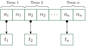
In general, we use lowercase Latin letters to denote polynomials, lowercase Latin letters with subscripts for coefficients, and corresponding lowercase Greek letters with subscripts for exponent vectors. Capital Latin letters with subscripts represent polyno-mial terms.
2.2.3
Arithmetic in a Polynomial Ring
For a ring to be a ring, it must have two binary operators, +, and×. For a polynomial ring these are called polynomial addition and polynomial multiplication, respectively. The operators are essentially the same for any polynomial ring, where polynomial addition (multiplication) relies on the addition operator (multiplication operator) of the base ring.
The addition of two polynomials is rather simple. For every like-term between the two polynomials, add their coefficients together and put this term in the sum, otherwise, put the same term in the sum as appears in the operands. Like-terms are terms which share the same monomial. Written more mathematically:
Definition 2.1 (Polynomial Addition)
Leta, b∈R[x1, . . . , xv], a=
Pna
i=1aiXαi, b=
Pnb
i=1biXβi be dense polynomials, such that we include zero coefficients. Further, let n= max{na, nb}, and prepend zeros to the polynomial which was smaller to make them equal length. Then:
a + b =
n
X
i=1
(ai+bi)Xαi
2.2. Algebra 15
The multiplication of two polynomials requires polynomial addition, and is es-sentially the sum of repeated distributions. Whether the polynomials are represented sparsely or densely, this scheme will work fine.
Definition 2.2 (Polynomial Multiplication)
Leta, b∈R[x1, . . . , xv], a=Pnai=1aiXαi, b=Pnbi=1biXβi then:
a × b =
na
X
i=1
nb
X
j=1
(ai×bj)Xαi+βj
!
The outer sum works as polynomial addition while the inner sum works more like building up terms of a polynomial — for a fixediand varying j,αi+βj are all unique. Note that
αi+βj is a component-wise summation as they are both multi-indices.
For division, it is more tricky. Finding an explicit formula for the quotient and remainder of two polynomials is not easy, but, an algorithm can easily define the process.
LetD be an integral domain and let a, b∈D[x] with b6= 0 and lc(b) be a unit in D. Let K be the field of fractions of D. Viewinga, b as polynomials in K[x] and since K[x] is a Euclidean domain, any pair quotient-remainder (q, r) in the Euclidean division of a
byb satisfy a = bq+r together withr = 0 or deg(r)<deg(b). It is not hard to verify that (q, r) is unique and that Algorithm 2.1 computes it. Moreover, Algorithm 2.1 shows that the coefficients ofq and r are actually in D. Therefore, the division with remainder of a byb, as polynomials inD[x], is well-defined.
Notice that we require the leading coefficient of the divisor to be a unit inD. When this is not the case, the division over the base ring elements, lc(c)/lc(b) is not usually defined (unless lc(b) exactly divides every coefficient in a, in which case we need not require lc(b) to be a unit). Moreover, since polynomials over integral domains and with positive degree are never units in their ring, then the polynomial division defined is es-sentially only for univariate polynomials. Multivariate division is much more interesting. It comes about as a consequence of Gr¨obner bases. Therefore, we leave its discussion to Section 2.2.4 regarding Gr¨obner bases.
Algorithm 2.1 polynomialDivision(a,b)
a, b∈D[x],a=Pni=0a aix
αi, b=Pnb i=0bix
βi,lc(b) is a unit inR;
returnsq, r∈D[x] whereqis quotient,rremainder, anda=qb+r,
deg(r)< deg(b).
1: r:=a
2: fori= 0tona−nbdo
3: ifdeg(r) =na−ithen
4: qi:=lc(r)/lc(b)
5: r:=r−qix(na−nb+i)b
6: else
7: qi:= 0
8: returnq=Pna−nb
i=0 qix(na−nb+i),r
When division is not possible due to the limitations of the base ring, such as when the divisor is not monic, there is still an option to perform pseudo-division.
Pseudo-division
Pseudo-division is a generalization of the idea of division with remainder on polynomials. The idea behind pseudo-division is to ensure that polynomial division occurs, if it can occur, without worrying about the restrictions of the base ring. In pseudo-division the division by the leading coefficient of the divisor is avoided entirely. Hence, neither do we require the divisor to be monic, the leading coefficient of the divisor to be a unit, nor that the polynomials be defined over an integral domain. Pseudo-division is defined for polynomials over any base ring [48]. Hence, this operation (while essentially univariate) can be defined for multivariate polynomials when they are viewed recursively.
Definition 2.3 (Pseudo-Division)
Leta, b, q, r ∈R[x], b6= 0, lc(b) =h, deg(a)≥deg(b). Then q is the pseudo-quotient and r the pseudo-remainder, satisfying the equation
hdeg(a)−deg(b)+1a = bq+r, deg(r)< deg(b).
Notice that the exponent on h is equivalent to the maximum number of division steps
that can occur. That is, the number of times one might actually perform a division in classical polynomial division. Therefore, this ensures the “division”4 of coefficients can
always occur. A classical algorithm for pseudo-division is shown in Algorithm 2.2. Notice that this algorithm is essentially the same as Algorithm 2.1 with the minor addition of multiplying by h at each division step.
4In implementation, one avoids multiplication byhand division entirely by simply ignoring both all
2.2. Algebra 17
Algorithm 2.2 na¨ıvePseudoDivision(a,b)
a, b∈R[x2, . . . xv][x1] =R[x], deg(b)>0;
returnq, r∈R[x] and`∈Nsuch thath`a=qb+r.
1: q:=0;r:=a
2: `:=0;h:=lc(b)
3: whiledeg(r)≥deg(b)do
4: k:= deg(r)−deg(b)
5: q:=hq+ lc(r)xk
6: r:=hr−lc(r)xkb
7: `:=`+ 1
8: return(q, r, `)
We also note that one can define alazy pseudo-division in the sense that the exponent on h is not exactly deg(a)−deg(b) + 1. Rather, the exponent is equal to the precise number of times one would need to multiply by h to make the division work. Of course, this has many practical benefits in implementation. Pseudo-division is discussed further in Section 4.4 with its practical implementation discussed in Section 4.4.1.
For more details and algorithms regarding polynomial arithmetic, see [48, Section 4.6] and [Sections 2, 6.12, and 25][31]
2.2.4
Gr¨
obner Bases, Ideals, and Reduction
The subject of Gr¨obner bases is a rich area within algebraic geometry, finding many theoretical and practical applications. It is concerned with, among many others, ideals. We refer the reader to [29] for a rather succinct description of Gr¨obner bases, and [6] for a more detailed description. A survey of the many applications of Gr¨obner bases can be found in [16].
We begin by defining ideals. An idealI is a subset of a ring R with the properties:
(1) ∀a, b∈I, a+b∈I
(2) ∀a∈I, r∈R, ar ∈I
If property (2) is not commutative, we can call I a right (or left, depending on which side r appears in (2)) ideal of R.
An ideal can be generated by a set of elements a1, . . . , an ∈R, denoted by: ha1, . . . , ani={a1r1+. . . anrn |r1, . . . , rn∈R}
and it is said that a1, . . . , an form the basis of the ideal or is the generating set of the ideal. IfA={a1, . . . , an}, a useful short-hand is to denoteha1, . . . , ani=hAi. It is worth noting that the same ideal can have many different generating sets.
Problem 2.1 (Ideal Membership Problem)
For an ideal I ⊆R and f ∈R, isf ∈I?
Gr¨obner bases yield a theoretically and computationally effective way of solving this problem. Simply, a Gr¨obner basis is special generating set of an ideal by which the ideal membership problem is easily solved. In order to formalize the solution to the ideal membership problem we must discuss reduction.
For the remainder of our discussion, we consider polynomials in the ringK[x1, . . . , xv] where K is a field. Gr¨obner bases are usually discussed in this context as all theorems and results hold in the case of a field. However, we note that it is still possible to work with Gr¨obner bases for multivariate polynomials over rings [1, Chapter 4]. Further, we must also fix some term order. We will see why this important. The particular one used is not of great importance, but it should remain fixed throughout. We use lexicographical ordering (see Section 2.2.2).
Reduction is simply a generalization of polynomial division. Letf, g, h, r∈K[x1, . . . , xv] be multivariate polynomials. It is said that f reduces to h modulo g in one step if and only if lt(g) divides some term, t of f with the result h being:
h=f − t
lt(g)g (2.1)
This reduction in one step is denoted:
f −→g h
Similarly, f reduces to h modulo g if and only if a sequence of reductions in one step produce h fromf. That is,
f −→g h1
g −→h2
g
−→. . .−→g h
This reduction is denoted:
f −→g +h
Moreover, we say a polynomial r is the remainder off with respect tog if f −→g + r
and r is reduced with respect to g. Where reduced means either:
(1) r= 0, or
(2) no terms ofr are divisible by the leading term of g.
2.2. Algebra 19
If we letq=t/lt(g) be the quotient from one reduction step, then we can accumulate a quotient from the many steps over an entire reduction, to obtain a full quotient alongside the remainder. Then, we get the following:
Definition 2.4 (Multivariate Polynomial Division with Remainder)
Leta, b, q, r ∈K[x1, . . . , xv], b6= 0. Then q is the quotient and r the remainder, satisfying the equation
a = bq+r, r is reduced with respect to b
We discuss our variation of multivariate division and its algorithms in Section 4.3
Reduction is more general than as has been described so far. Reduction in its full form replaces g by a set of polynomials G = {g1, . . . , gn}. Thus, it is also sometimes referred to as multi-divisor polynomial division. If there were not enough synonyms already, the remainder of a multi-divisor polynomial division is also called a normal form. We discuss this in Section 4.5.
We sayf reduces tohmoduloGif and only if there exists a sequence, say (i1, . . . , im), of reductions in one step, using one of gi ∈G for each step.
f gi1 −→h1
gi2 −→h2
gi3
−→. . .−→gim h
f −→G +h
We note that not every polynomial in G must be used for a reduction, and, it is very possible to use the same polynomial several times. In the case of multiple divisors, a polynomial r is reduced with respect to Gif either:
(1) r= 0, or
(2) no terms ofr are divisible by lt(gi) for every gi ∈G.
From this, we can see why it is important to fix a term order when discussing reductions. As we need to decide the leading term of the divisor, this changes depending on the term order used. Moreover, the term order then impacts the decision of whether a polynomial is reduced or not.
For example, under lexicographical ordering, the polynomialf =x2+xy4 is reduced
with respect tog =x3+xy3 becausex3 does not divide eitherx2 orxy4. However, under
degree lexicographical ordering, f =xy4 +x2 and g =xy3 +x3 and now f is no longer reduced with respect to g asxy3 divides xy4.
A similar problem occurs with multiple divisors. Let f = x2y, G = {g1, g2} with
g1 =x2 and g2 =xy−y2,
and yet both 0 and y3 are reduced with respect to G. Clearly, the order in which the
divisors are applied makes a difference. So, reduction is an ambiguous problem. At least, that is the case when the divisor set is a general set of polynomials.
This is troublesome. Particularly because one solution to the identity membership problem is the following: for G={a1, . . . , an} and hGi=I ⊆R,f ∈R,
f −→G + 0 =⇒ f ∈I.
Since the order of application influences the final result, we cannot say the converse, that if f ∈ I then f −→G + 0. However, Gr¨obner bases give us just that. They are special
sets such that that the process of reduction with respect to them always yields a unique remainder. Therefore, if G is a Gr¨obner basis then
f −→G +0 ⇐⇒ f ∈I.
This if and only if relation is a very important property of Gr¨obner bases. Algorithm 21.33 in [31] shows that every ideal admits a Gr¨obner basis, and it can be computed ef-fectively. Hence, these bases allow effective and practical solving of the ideal membership problem, among many other problems. See Chapter 21 in [31] and all of [16] for many other such problems and applications.
2.2.5
Algebraic Geometry
Here, we give only a very brief review of some definitions which will become useful in later theorems. In particular, we are interested in hyperplanes, hypersurfaces, and their degrees.
An ordinary 2-dimensional surface exists in a 3-dimensional space. A hypersurface is just a generalization of a surface to arbitrary dimension. Consider a space — usually affine or Euclidean, the particulars of which are not important — of dimension n, say
Kn. This is the ambient space. Then, hypersurfaces are sub-spaces of dimension n−1.
Equivalently, they have codimension 1 with their ambient space.
Hypersurfaces are defined by a single polynomial inK[x1, . . . , xn] =K[X] asp(X) = 0. A hypersurface is said to have degree d if the polynomial defining it has total degree
d. A hyperplane is simply a hypersurface of degree 1. For example, the hypersurface
defined by p(x, y, z) = 2x2yz+ 3xz+y= 0 is a hypersurface of degree 3 in
K3, with the
ambient space being K4.
2.2. Algebra 21
2.2.6
(Numerical) Linear Algebra
Beyond the very basics of linear algebra, like vectors, matrices, and systems of equations (with which we assume the reader is familiar), linear algebra is a very broad topic, even compared to algebra as a whole. Here, we only highlight a specific topic which some may not be familiar.
Given a matrix, A ∈ Rn×m, a singular value decomposition (SVD) of A is a fac-torization into the form UDVT where U ∈ Rn×n, V ∈
Rm×m are orthonormal and D ∈Rn×m =diag(σ
1, σ2, . . . , σp), p=min{n, m}. The diagonal entries of D are known as the singular values of A. Generally, algorithms produce D such that the singular values appear in a decreasing order, with σ1 ≥ σ2 ≥ · · · ≥ σp ≥ 0 [22]. The diagonal matrix of the SVD gives the rank of A as r:
A=UDVT =U
σ1 . .. σr 0 . .. 0 VT
If A is of full rank then r=p=min{m, n}. Otherwise, σr+1 =· · ·=σp = 0.
In numerical analysis, the singular value decomposition of a matrix provides a great deal of information regarding the (numerical) properties of the matrix, such as, effective rank, nearness to singularity, and the matrix’s condition number [32]. Whereas the actual rank of a matrix is given as the number of non-zero singular values, if σr+1, . . . , σp are very small but non-zero then it is possible to say that A is numerically rank deficient. This is important as the condition number of A — a measure of the sensitivity of a problem to numerical errors and perturbations — is given by κ(A) = σ1
σp. Of course, if
σ1 σp ≈0 then the condition number will be very large and the ill-conditioning of A may cause drastic errors in further computations [22]. Thus, it can then be convenient to explicitly set σr+1 =· · ·=σp = 0 and regard A as rank-deficient, with rank r.
2.3
Representing Polynomials
For the sake of representing polynomials effectively there are two aspects to consider. Algorithms operating on these polynomials can be evaluated by their running time and/or memory usage. Generally, they work inversely, in the sense that more memory means the algorithm can run more quickly (in theory) while using less memory requires more steps from the algorithm. This interplay is an important consideration, especially considering the memory configuration of modern computers (see Section 2.1). Ideally, we want both time and memory to be minimized.
Let us begin with an example: addition of two univariate polynomials. Let a, b ∈
R[x] such that
a=anxn+an−1+xn−1 +· · ·+a1x+a0 =
n
X
i=0
aixi (2.2)
b =bmxm+bm−1+xm−1+· · ·+b1x+b0 =
m
X
i=0
bixi (2.3)
In this representation, which we call adense representation, notice that the indices of the coefficients match the exponent of their associated monomial. All terms are represented regardless of the value of its coefficient, in particular, terms with a 0 coefficient. This provides advantages for notations and computation. Assumingn =m (otherwise, simply extend the smaller polynomial by adding zero terms so that the sizes match) then the addition, a+b is simply:
a+b = n
X
i=0
(ai+bi)xi.
In contrast, for a sparse representation, it is not as simple as matching indices and adding coefficients, one must also match monomials, requiring more computational steps within the algorithm.
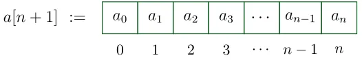
Consider a possible implementation of this dense univariate representation. An obvious solution is to encode each polynomial as simply an array of coefficients. In this scheme, the exponent on the monomial corresponding to each coefficient is implied by the coefficient’s index (Figure 2.1) A polynomial addition algorithm in this representation is dead simple; it is nothing more than iterating through two arrays, summing corresponding indices. In this dense array representation, one can also immediately query things such as leading monomial, leading coefficient, number of terms, and degree.
a[n+ 1] := a0 a1 a2 a3 · · · an−1 an
0 1 2 3 · · · n−1 n
2.3. Representing Polynomials 23
Consider however, encoding the polynomial x10000 −1 in this dense array
repre-sentation. Although there are only four defining items (coefficients 1 and -1, and the monomials x10000 and x0) we would need to create an array of size 10001 to encode the polynomial. Moreover, if this polynomial was used in some algorithm, say polynomial addition, much of the time of the algorithm would be spend summing coefficients where at least one operand was 0, a very wasteful operation.
This leads to the discussion of the sparsity of a polynomial itself5. In this sense, a
polynomialis dense or sparse regardless of how it is represented. One says a polynomial is sparse if it has relatively few non-zero terms compared to the maximum number of terms possible for a polynomial with the same degree. Similarly, a polynomial is dense if it has relatively few zero terms.
A polynomial can either be represented densely or represented sparsely, regardless of whether it is dense or sparse. Naturally, sparse representations work best when they are used to represent sparse polynomials. The same goes for dense.
Of importance here, is deciding how to represent multivariate polynomials. For a fixed maximum partial degree, the number of multivariate polynomial terms increases exponentially in the number of variables. Even with a partial degree of no more than 2, multivariate polynomials in 3 variables have up to 27 terms while 10 variables already have up to 59049 terms. A dense representation would have to encode at least that many terms, a prohibitively large number as degrees and number of variables increase. How-ever, multivariate polynomials are rarely dense in computer algebra problems. Generally speaking, multivariate polynomials are sparse, either with many variables, each of low degree, or a few variables, each of high degree but very few non-zero terms [26].
Mathematically, we can write sparse polynomials using summation notation as well, with slightly different notation. This is the same notation as was presented in Sec-tion 2.2.2, which we repeat here for completeness.
a =
na
X
i=1
aixe11i. . . xeviv = na
X
i=1
aiXαi
In this summation notation, the na terms are sorted decreasingly according to lexico-graphical ordering. ai ∈ R is theith coefficient, and e1i, . . . , evi are exponents of the ith monomial. To simplify notation, often a multivariate monomial will be written as Xαi, where a capital letterX denotes the sequence of variablesx1, . . . , xv andαi =e1i, . . . , evi is a v-tuple or multi-index of exponents. We leave the discussion on the implementation of sparse representations to Chapter 3, where many details and implementation strategies are discussed.
Lastly, the idea of a recursive representation should not be forgotten. That is, rep-resenting a multivariate polynomial p∈R[x1, . . . , xv] explicitly as p0 ∈R[x2, . . . , xv][x1].
5The sparsity of a polynomial can depend on the basis in which it is represented. In general, we use
This representation is very useful computationally when wishing to perform essentially univariate operations on a multivariate polynomial. For example, pseudo-division (Sec-tions 2.2.3 and 4.4), greatest common divisor, content and primitive part[31, Section 6.2], and subresultants [31, Section 6.10] are all essentially univariate operations.
We can easily define such a representation, again in summation notation, as:
f(x1, x2, . . . , xv) = n
X
i=1
gi(x2, . . . , xv) · xi1
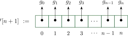
This representation is tricky to implement in the sense that coefficients are themselves polynomials. However, it is also essentially univariate in its representation. Thus, it could be convenient to use a dense representation, like arrays, where the index implies the exponents on the main variable (x1) and the entries in the array are the polynomial
coefficients (gi(x2, . . . , xv)). In a C-like programming language the coefficients in the array could just be pointers to other polynomials, such as in Figure 2.2. We discuss our more efficient recursive sparse implementation in Section 3.4.
f[n+ 1] := · · ·
g0 g1 g2 g3 gn−1 gn
0 1 2 3 · · · n−1 n
Figure 2.2: Array representation of a dense recursive multivariate polynomial.
For further discussion on polynomial representations in various computer algebra systems, [26] provides a good overview. For a detailed look at the implementations and representations of Mapleand Singularsee [60].
2.4
Working with Sparse Polynomials
As we saw in the last section, dense polynomial representations provide some compu-tational advantages, such as very simple algorithms and the ability to instantly query information like degree, number of terms, and coefficients at a particular index. Many of these advantages are lost when working with sparse representations.
Without even considering implementation, one can see the difficulties of working with sparsely represented polynomials. Consider the question does this polynomial contain the monomial xd, for some d. In a dense representation, p = Pn
i=0pix
i, the answer is immediate: does pd = 0? For a sparse representation, p =
Pn i=1pix
2.4. Working with Sparse Polynomials 25
match indices and add those corresponding coefficients. Arithmetic in general is more cumbersome for a sparse representation.
So why do we care about sparse polynomials? The short answer is memory. Com-puter memory is almost always the limiting factor. Historically, the amount of memory available limited the size of problems that computers could solve and how they solved them. Today, this is less of a concern. On modern architectures we are more concerned with how memory is used (Section 2.1).
Many algorithms were still (and are) developed for dense representations [48, Sec-tion 4.3.3 (How fast can we multiply?)]. Methods like Karatsuba [46], Toom-Cook [12], and Sch¨onhage-Strassen [69] have been developed that are asymptotically very fast. How-ever, for sparse (multivariate) polynomials, whose dense representations are prohibitively large, these algorithms are ineffective. Moreover, considering the processor-memory gap, we would like to maintain good cache-complexity for sparse polynomials, which is impos-sible if they are represented densely. Hence, we want to work with sparse polynomials represented sparsely.
Two very important works which focused on sparse polynomials considered their arithmetic [42] and their interpolation [76]. Sparse polynomial arithmetic in [42] was left unnoticed for many years, until its rediscovery in the late 2000s by Monagan and Pearce [56, 58, 59]. These algorithms for sparse arithmetic can be adapted to modern architecture with good cache complexity. Indeed, this is the main subject matter of Chapter 4. Here, we present the original sparse algorithms of [42] as a base to work from and to refer to later. Sparse interpolation is left to the discussion of Section 5.3.
The ideas of sparse arithmetic are built up in succession. Division relies on multi-plication; multiplication relies on addition. We begin with addition. Let us fix the two operands of a binary polynomial operation as a and b with the result beingc.
a= na
X
i=1
aiXαi b= nb
X
j=1
bjXβj c= nc
X
k=1
ciXγk
Addition (or subtraction) of two polynomials requires joining the terms of the two sum-mands, combining like-terms (with possible cancellation) and then sorting the terms of the sum. Sorting is necessary in this case in order to maintain a canonical representation — an issue which will come up again for every operation. A na¨ıve approach is to compute the suma+b term-by-term, adding a term of the addend (b) to the augend (a), inserting it in its proper position among the terms ofa so that the term order is maintained. One could think of this as analogous toinsertion sort.
This method is inefficient and does not take advantage of the fact that both a and
or difference of coefficients is computed), with the output being automatically sorted. This algorithm is presented in Algorithm 2.3. Subtraction is essentially the same by only replacing the addition of like-term coefficients with their subtraction.
Algorithm 2.3 addPolynomials(a,b)
a, b∈R[x1, . . . , xv], a=Pni=1a aiXαi, b= Pnb
j=1bjXβj;
returnc=a+b=Pnc
k=1ckXγk∈R[x1, . . . , xv]
1: (i, j, k) := 1
2: whilei≤nandj≤mdo
3: ifαi< βjthen
4: ck :=bj
5: γk :=βj
6: j:=j+ 1
7: else ifαi> βjthen
8: ck :=ai
9: γk :=αi
10: i:=i+ 1
11: else
12: ck:=ai+bj
13: γk:=αi
14: i:=i+ 1
15: j:=j+ 1
16: ifck= 0then
17: continue #Don’t incrementk
18: k:=k+ 1
19: end
20: whilei≤ndo
21: ck:=ai
22: γk:=αi
23: i:=i+ 1
24: k:=k+ 1
25: whilej≤mdo
26: ck:=bj
27: γk:=βj
28: j:=j+ 1
29: k:=k+ 1
30: returnc=Pk `=1c`Xγ`
Much like addition, polynomial multiplication requires generating the terms of the product, combining like-terms among the product terms, and then sorting the product terms. A na¨ıve approach is to compute the product a·b by distributing each term of the multiplier (a) over the multiplicand (b), combining like terms, and sorting: c = a·b = (a1Xα1 ·b) + (a2Xα2 ·b) +· · ·. This is inefficient because all nanb terms are generated, whether or not they combine as like-terms. Also, the finalnanb terms must be sorted.
2.5. Interpolation & Curve Fitting 27
a·b=
(a1·b1)Xα1+β1 + (a1·b2)Xα1+β2 + (a1·b3)Xα1+β3 +. . .
(a2·b1)Xα2+β1 + (a2·b2)Xα2+β2 + (a2·b3)Xα2+β3 +. . . ..
.
(ana·b1)X
αna+β1+ (a
na·b2)X
αna+β2+ (a
na·b3)X
αna+β3+. . .
We can consider this like an na-way merge sort, where at each step, we select the maximum term from the heads of the streams and use it at the next term in the product, removing it from the stream in the process. The new head of the stream where a term is removed is then the term to its right. To be computationally effective in implementation, the product (ai ·bj)Xαi+βk is only actually computed when it is removed from a stream (see Section 4.2.1 for implementation details). If there is no unique maximum, then the maximums are all like-terms and we can select all such terms and add their coefficients together to form a single term of the product. This is shown in the algorithm (Algo-rithm 2.4) by accumulating sums of products in ck (line 16), and only updating k when the maximum degree “drops” and the resulting coefficient is non-zero (line 11).
We use a variable to keep track of the index of the head of each stream, and do a brute-force search over the those heads for the maximum. We use the variable fs to give the “column” index of each stream, where s is the index of the row (stream). Thus, fs picks out the current head element of stream s. Further, we use the index I to denote the index of the first non-empty stream. In this na-way merge, since we have
Xαi+βj > Xαi+1+βj and Xαi+βj > Xαi+βj+1, then the streams will become “empty” in order of increasingai. MaintainingI provides advantages for notation and computations.
The last of the arithmetic operations discussed in [42] is exact division. Division is a direct application of multiplication. In fact, it is simply formulated as a multiplication in which one of the operands is continuously updating. We explain it fully in Section 4.3 where it is extended to division with remainder. We also expand on the rather terse original presentation of the algorithm.
2.5
Interpolation & Curve Fitting
6Interpolation has a long history with many applications. Arguably, the history of inter-polation is more rich in numerical analysis but, nonetheless, it is fundamental to both symbolic and numeric computation. Precisely, interpolation is the process of, given a set of (possibly multivariate) points, πi, and values, βi, finding a function, f, such that
f(πi) = βi. In essence, interpolation is the process of transforming a set of discrete data points into a function. This function may be the exact function which produced the data
6The unpublished work of George Miminis,Introduction to Scientific Computing, is to thank for the