DYNAMIC RELATIONSHIP BETWEEN EXCHANGE RATE OF BRICS COUNTRIES: CAUSALITY AND CO-INTEGRATION ANALYSIS

(1)

96

International Journal in Management and Social Science

http://ijmr.net.in, Email: [email protected]

Dynamic Relationship between Exchange Rate of BRICS Countries: Causality and

Co-Integration Analysis

Prof. Dr. Neera Verma

Department of Economics, kurukshetra university kurukshetra, (India) &

Amandeep Kaur

Assistant Professor in Economics, Department of Economics, B.A.R. Janta College, Kaul

Abstract: Exchange rate is an important element of the country’s economic health. Exchange rate fluctuations affect the value of international investment portfolios, Competitiveness of exports and imports, value of international reserves, currency value and balance of payment. In the past few decades, some large economies such as Brazil, Russia, India, China, and South Africa (BRICS) have acquired a vital role in the world economy as producers of goods and services, receivers of capital, and as potential consumer markets. The aim of this study is to explore the dynamic relationship between the FXR of BRICS nations using time series data running from 1991-92 to 2017-18. Our paper measures the volatility from the changes in the foreign exchange rate of emerging market economies and analysis the Co integration, Granger Causality analysis, variance decomposition analysis and impulse response function. In this research, Augmented Dickey-Fuller (ADF) and Phillips-Perron (PP) unit root tests are applied to test stationarity of data and the data was found stationary at first difference. Karl Pearson correlation test was used to find the correlating relationship between foreign exchange rates of BRICS nations are significantly correlated with each other. Johansen's cointegration test is applied to determine the long-run equilibrium relationship between the study variables. Granger causality test is employed to determine the causality and often adopted the local projections approach to derive impulse response functions and variance decomposition analysis, variance decompositions serve as tools for evaluating the dynamics interactions and strength of causal relations among variables in the system. We find that the co-integration test confirmed that FXR of BRICS nations are co integrated, indicating an existence of long run equilibrium relationship. The Granger causality test confirmed the presence of two way causality betweenFXR India and FXR Brazil. The results further indicate that there is one way causality between FXR Russia <= FXR INDIA and FXR South Africa <= FXR India.The empirical results of both variance decomposition analysis and impulse response function exhibits that foreign exchange rate of BRICS nation are not independent each other.

Keywords: Time series, Volatility, exchange rate

INTRODUCTION

“It is not an overstatement to say that real exchange rate behaviour now occupies a

central role in policy evaluation and design”Edwards (1994).

1.1 Introduction: Foreign exchange rate as generally defined in economic literature is the rate at which one country‟s currency can be traded for another country‟s currency. While

(2)

97

fixed exchange rate policy and the flexible exchange rate policy. By fixed exchange rate policy (regime), the exchange rate is set and government is committed to buying and selling its currency at a fixed rate, while flexible exchange rate policy defines a situation when the exchange rate is set by market forces (demand and supply for a country‟s currency).

Exchange rate volatility hinders the flow of international trade and Flexible Exchange Rate system. Volatility of the exchange rates of developing countries is one of the main sources of economic instability around the world. Exchange rate volatility is defined as the risk associated with unexpected movements in the exchange rate. Exchange rate volatility is a measure of the fluctuations in an exchange rate. It is also known as a measure of risk (Kamble G. and Honrao P., 2014). The currencies of many emerging and developing economies suffered large depreciations with the onset of the global financial crisis. Most of the BRICS economies have undergone depreciation and have shown volatility, coinciding with the world economic and financial conditions.

1.2 BRICS GROUP: THE GOLDMAN SACHS REPORT

The concept of BRIC was introduced in the year 2001 by Jim O‟Neill, then chairman of

Goldman Sachs, one of the biggest investment management companies in the world explain the term of BRIC in a paper titled „Building Better Global Economic BRICs‟1. According to one of the earliest reports (2001) on emerging and dynamically growing economies by Goldman Sachs - Brazil, Russia, India and China were suggested to merge into that special “economic union”. It took into account the total land area of BRIC members, population,

GDP, potential of the consumer markets as well as influence within their respective regions. It was concluded that over 10 years, the share of the BRIC countries and especially China in world GDP will grow, raising important issues about the global economic impact of fiscal and monetary policy in the BRIC countries. In 2003, their report, “Dreaming with BRICs: The Path to 2050”2

stated that by 2050 these economies together would be larger in US Dollar terms than the G-6 consisting of the United States, Germany, Japan, the United Kingdom, France and Italy. In 2009, BRIC countries held their first summit. In 2010, South Africa was invited to join – thus transforming BRICs into BRICS (Oehler-Sincai, 2011). South Africa was added to the list on April 13, 2011 creating “BRICS”.

1

Goldman Sachs, Building Better Global Economic BRICs, Global Economics, 66, 2001, http://www.goldmansachs.com/our-thinking/topics/brics/brics-reports-pdfs/build-better-brics.pdf.

2

(3)

98

http://ijmr.net.in, Email: [email protected] Table: 1.1 Currency and Current Exchange Rate System of BRICS Nations

Country Currency Current Exchange Rate System

Brazil Real Floating Exchange Rate

Russia Ruble Free Floating Exchange Rate

India Rupee Floating Exchange Rate

China Yuan Managed Floating Exchange Rate

South-Africa Rand Floating Exchange Rate

Source: IMF (2015)

Exchange rate volatility plays a significant role in this financial globalization process. So as to manage this process effectively, it is very important for the policy makers and various agents to be able to generate accurate forecasts of exchange rates and their anticipated volatilities. Thus, it would be of great importance to investigate whether established time series models, econometric models or a combination of both models perform equally well for emerging and frontier countries.

Focus of This paper on behavior and volatility of foreign exchange rate. The research paper has been divided into five Sections. The first Section devoted to the Survey of literature for foreign Exchange Rate determination, behavior, volatility and forecasting of foreign exchange rate and section-II analyze the objectives, data sources, methodology, econometric modelling approach and hypothesis. Section - III is related to the empirical analysis of behavior, volatility and forecasting of foreign exchange rate in BRICS nations. Section-IV explained the empirical estimation of causality analysis of foreign exchange ratefrom 1991-2017 and Section-V presents the Main conclusions and policy implications of this study.

SECTION-I

Review of Literature

1.3 Volatility and Forecasting of Exchange Rates via Time Series Models: BRICS

Nations

(4)

99

1.3.1 Empirical Evidence of the Exchange Rate Behaviour and VolatilityApplications in

BRICS Countries: To analyse the behaviour of foreign exchange rate and investigate the Volatility in foreign exchange rate(s) in BRICS countries over study period i.e. 1990-2016. This section covers a broad and comprehensive review of the literature on foreign exchange rate volatility and using different measures of exchange rate volatility. This observed that greater exchange rate volatility generates uncertainty thereby increasing the level of riskiness of trading activity and this will eventually depress trade. Therefore, this issue became an interesting research question for many economists that embarked themselves into the formulation of theories. The literature on modelling or forecasting exchange rate volatility uses ARCH, GARCH, FIGARCH, E-GARCH models. Each of these contributions to the ARCH family has concentrated on refining both the mean and variance equations to better capture the stylised characteristics of the time series. The standard class of ARCH family models has certainly been extensively applied to exchange rate data, see, for Bollerslev (1990), Engle and Gonzalez-Rivera (1991), Mundaca (1991), Higgins and Bera (1992), Drost and Nijman (1993), Bollerslev and Engle (1993), Neely (1993), West and Cho (1995), Byers and Peel (1995), Hu and Tsoukalas (1999),Johnston and Scott (2000), Kazantzis (2001), Chong et al. (2002), Mapa (2004), Alberg et al. (2006), Hussein and Jalil (2007), Umar (2010), Chortareas et al. (2011), Vee et al. (2011) and Pacelli (2012).

There are researchers use the model by Koray and Lastrapes (1989), Kroner and Lastrapes (1990), Chowdhury (1993), Calvo, Leiderman and Reinhart (1993), Pesaran, Shin and Smith (2001), Mustafa and Nishat (2004), Todani & Munyama (2005), Guangling Liu (2007), Berger et al. (2008), Dua and Sen (2009), Bal (2012), Danqing Wang (2012), Erdal et al. (2012), Pujula (2013), Yadav (2014), Ajao (2015) and Yu hsing (2016). Edwards (1996, 1999) find that real exchange rate volatility causes countries to prefer more flexible regimes and relationship is established the coefficient of exchange rate volatility is either negative or positive with economic variables.

(5)

100

volatility and trade on the premises that exchange rates cluster in period of high or low volatility (i.e. time-varying conditional volatility). It‟s found a small but significant effect of exchange rate volatility on trade and observed that this effect varies across the countries. Chowdhury (1993) investigated the impact of exchange rate volatility on the trade flows of the G-7 countries in context of a multivariate error-correction model. They found that the exchange rate volatility has a significant negative impact on the volume of exports in each of the G-7 countries. Edwards (1999a) has analysed the impact of capital flows on the exchange rate for Latin American and Asian countries and find that an increase in capital flows cause the exchange rate to appreciate. However, the degree of appreciation or the strength of the relation between capital flows and the exchange rate may vary across countries and time. Mustafa and Nishat (2004) have investigated the effect of exchange rate volatility on export growth between Pakistan and other leading trade partners such as SAARC, ASEAN, European and Asia Pacific regions. They found that exchange rate volatility had negative impact on export flows of Pakistan with United Kingdom, United States, Australia, Bangladesh and Singapore. While in the case of India and Pakistan, there exists only long-run impact and no short run relationship. In the case of New Zealand and Malaysia, no relationship was found. Todani & Munyama (2005) examine the characteristics of short-term fluctuations/ volatility of the South African exchange rate and investigates whether this volatility has affected the South Africa‟s exports flows. This paper

investigates the impact of exchange rate volatility on aggregate South African exports flows to the rest of the world, as well as on South African goods, services and gold exports.

(6)

101

and find that an increase in capital inflows and their volatility lead to an appreciation of the exchange rate. Sharma (2011) tried to find relationship between the volatility in exchange rate in the spot market and trading activity in the currency futures. In analysis conducted using Granger causality test, ARCH and GARCH model, he found that volatility of spot exchange rate after the introduction of currency futures is greater than volatility of spot exchange rate before the introduction of currency futures. Bal (2012) has examined the effects of exchange rate volatility on India's export and found no statistical and significant relationship between the exchange rate volatility and export of the country. But, the short term disequilibrium of exchange rate was negatively affects the export of the country.

Wang (2012) analysis of is aimed that exploring the relationship between exchange rate volatility and foreign direct investment in selected emerging economies, specifically, Brazil, Russia, India, and China (BRIC). The sample of data was selected over the period of 1994-2012 for both exchange rate volatility and foreign direct investment for all countries. The standard deviation of monthly exchange rate changes is applied to examine the exchange rate volatility and its influence upon foreign direct investment using an Autoregressive Distributed Lag (ARDL) approach and the Cointegration and Error Correction Model Erdal et al. (2012) studied the effect of real effective exchange rate volatility on agricultural exports and imports. REERV were estimated by a GARCH (1, 1). The authors implemented Johansen‟s (1991) procedure to test for co-integration and estimate long-run relationships.

The direction of the effect was determined using pairwise granger causality tests. The authors found a positive effect of exchange rate volatility on exports, while the effect was negative for imports. Pujula (2013) estimated a Multivariate GARCH-M model with the mean equation specified as a VAR model of two variables exports and exchange rates. The author found positive own country volatility effects and negative third country volatility effects (EUR/USD) on Ghanaian total exports. Similarly, Grier and Smallwood (2013) applied a Multivariate GARCH-M and specified the mean equation with three variables growth rates of exports, foreign income, and the real exchange rate. His findings support negative effects of real exchange rate volatility on exports from both developed and developing countries. Yadav (2014) investigate the impact of exchange rate system on foreign trade of a country. In this study we will see how foreign exchange volatility impact on a country‟s

(7)

102

Ajao (2015) examined the determinants of real exchange rate volatility in Nigeria from 1981 through 2008. The volatility of exchange rate was obtained through the GARCH (1, 1) technique and the ECM was used. The co-integration analysis reveals the presence of a long term equilibrium relationship between REXRVOL and its various determinants. The empirical analysis further revealed that openness of the economy, government expenditures, interest rate movements as well as the lagged exchange rate were among major significant variables that influenced REXRVOL during the period. The study therefore recommended that the central monetary authority should institute policies that will minimize the magnitude of exchange rate volatility while the federal government exercise control of viable macroeconomic variables which may have direct influence on exchange rate fluctuations. Yu hsing (2016) analysed the determinants of the South African rand/us dollar (ZAR/USD) exchange rate based on demand and supply analysis and applying the EGARCH method, the paper finds that the ZAR/USD exchange rate is positively associated with the south African government bond yield, US real GDP, the US stock price and the south African inflation rate and the 10-year US government bond yield, south African real GDP, the south African stock price, and the US inflation rate negatively influenced. The adoption of a free floating exchange rate regime has reduced the value of the rand vs. the US dollar.

Forgoing review of literature indicates that there has been no systematic study with regards to volatility the analysis and interdependence of FXR of the BRICS nations. The present work is modest attempt to of his research gap. In order to fulfil this gap, the present study was undertaken.

Section-II

Objectives, Data Sources and Methodology

1.4 Objectives of Study: 1. To analyses the behavior of Exchange Rate in BRICS nations and empirically find out the volatility of Foreign Exchange Rate (FXR) in BRICS nations. 2. To explain the causality and co-integration of Foreign Exchange Rate (FXR) of BRICS nations with each other

The paper deals with reasons for appreciation or depreciation of currency followed by exchange rate determination. The present research tests validity of this hypothesis in association with the exchange rate of the BRICS Nations in form of the US dollar because US is the single largest trading partner of BRICS and it is the major international currency. 1.5 Data and Variables: The analysis is based on panel data for BRICS nation

(8)

103

1991 to 2017 to analyse the exchange rate determination in BRICS nations.

DATA SOURCES: The BRICS data for the period 1990-2017 has been collected from various secondary sources from various publications at national or international level. Such as Statistical data base of IMF, World Bank, UNCTAD and UNO. The information has also been collected from official websites of respective Government/ World Bank/ IMF and Central Banks of BRICS countries, etc.

 IMF's (International Monetary Fund) International Financial Statistics (Various Issues), 1980-2017.

 UNCTAD (United Nations Conference on Trade and Development) Various Issues

 World Bank Publications of World development indicators (Various Issues).

 Penn World Table (PWT) & Global Financial Data (GFD).

 UN's (United Nations), Year Book of International Trade Statistics.

 World Currency Yearbook (WCY) & World Economic Outlook (WEO).

 IMF Annual Report on Exchange Arrangement and Exchange Restriction, various issues.

 Federal Reserve Bank of St. Louis. (Fed World www.fedworld.gov)

Research Methodology

1.6 Econometric Modelling Approach: During the literature review and based on the research gaps, the following research questions have been identified that need to be answered through this research work. By keeping the above cited views in mind, the researcher has framed the following objectives, Research Questions and hypotheses for the purpose of present study.

Fig. 1.1: Research Methodology for Objectives

IDENTIFY SET

OF KEY RESEACRH VARIABLES

FROM LITERATURE

SURVEY

(9)

104

http://ijmr.net.in, Email: [email protected] 1.6.1 RESEARCH METHODOLY: TIME SERIES ANALYSIS:

The researcher has used following statistical and econometrics tools with respect to above mentioned objectives:

1. Descriptive Statistics: The descriptive statistics of the data applied in the study are explained in details in this section. Taking into account the fifth assumption of the classical linear regression model, there is a prediction which assumes that the disturbances of the data must be normally distributed, thus, the need to look into the skewness and kurtosis behaviours of the data. Statistically, a normally distributed data is known to be not skewed and also must have a kurtosis of 3.

2. Unit Root Test: The data pertaining to the study of foreign exchange rate and selected variables is time-series data and time-series data has some distinguished features which require some understanding before putting it to some statistical treatment and further analysis. One such feature of time-series data is its "stationary”. A time-series is said to be stationary if its mean and variance are constant over time and the value of the covariance between the two time periods depend only on the lag between the two time periods and not the actual time at which the covariance is computed".

There are a number of ways through which stationary of time-series could be studies. Then methods include graphical presentation of time-series data, deriving an According function (ACF) and correlogram, and by applying Unit Root tests. There are a number tests which are being used widely to detect Unit Root of a time-series like Dickey-Fuller and Augmented Dickey-Fuller test developed by Dickey and Fuller (1979, 1981), Phillips Perron test (Phillips and Perron, 1988) and Kwiatkowski-Phillips-Schmidt-Shin (KPSS) and (Kwiatkowski et. al, 1992).In this study, Graphical Presentation method as well as Unit Root tests have been sorted order to check stationary status of time-series data. The most popular among all Unit Root tests, Augmented Dickey-Fuller test has been applied for detection of a Unit Root supplemented by Phillips-perron test.Augmented Dickey-Fuller (ADF), Philips-Perron(PP) test are used in this study to test the presence of unit root problem in the time series data. If the time series data is non-stationary in levels, it should be stationary in first difference with the same level of lags.

Test of stationary that has recently become popular is known as the unit root test. This test is to consider the following model:

Yt = Yt-1 + ut

Where ut is the stochastic error term that follows the classical assumptions, namely, it has zero

(10)

105

The hypothesis are formulated as follows:

H0 : Yt = I (1) VS H1 : Yt = I(0)

Dickey-Fuller Unit Root Test:

Null Hypothesis  Ho :  = 0 (Unit Root Problem)

Alternative Hypothesis  Ho:  ≠ 0 (No Unit Root Problem)

There are three type of DF methods to check unit root problem. Model-1 Without Constant and Trend

ΔY= δ Y(t-1)+ εt

Model-2 With Constant

ΔY=α+ δ Y(t-1)+ εt

Model-3 Without Constant and Trend

ΔY=α+δ Y(t-1)+ βT+ εt

Decision rule:

If t* > ADF critical value ⇒ not reject null hypothesis, i.e., unit root exists. If t* < ADF critical value ⇒ reject null hypothesis, i.e., unit root does not exist.

3. Augmented Dickey Fuller test: A lacuna of this test is that the presence of Autocorrelation in the

residual term may distort the critical values used in the hypothesis testing which may give spurious

results. To overcome this problem Dickey and fuller (1981) suggested Augmented Dickey-Fuller test

(ADF) which has been applied in this study. For the remove the autocorrelation problem we adopted the

Augmented Dickey Fuller (ADF) Test.

Augmented Dickey-Fuller (ADF) is a one-sided test which is based upon following hypothesis:

H_(0 ): γ=0 VS H_1: γ<0

It is a test for unit root in a time series sample developed by Dickey and Fuller (1981). The augmented Dickey-Fuller (ADF) statistics, used in the test, is a negative number. The more negative it is, the stronger the rejection of the hypothesis that there is a unit roots at some level of 5 percent confidence. ADF test follows the below stated model:

Augmented Dickey Fuller Test:

ΔYt= α + βt + γYt-1 + βt ΔYt-1 + …+ δpΔYt-p + εt--- ()

Where α is a constant, β the coefficient on a time trend and p the lag order of the autoregressive process. Imposing the constraints α = 0 and β = 0 corresponds to modeling a random walk and using the constraint β = 0 corresponds to modeling a random walk with a drift. By including

(11)

106

http://ijmr.net.in, Email: [email protected] ∆Yt=a+T + yt-1 + i yt-i +ui ……….()

If the calculated values of γ are less than the critical values then the Null hypothesis could not

be rejected which may conclude that the FXR time series is non-stationary.

If Time series data is Non-Stationary then to data convert to stationary we use the In this situation use the DSP to get stationary time series.

With Constant

(yt ) = Q + yt-1 + ct

With constant and trend

(yt ) =  +  + yt-1 + ct

The Critical values depend upon the lag length chosen and whether a drift term or trend component is included or not in the above regression. It is preferred to not allow too many lags in ADF equation in order to maintain the strength of regression. Selecting an optimal lag is an empirical question. Therefore, optimal lag length has been selected by using Schwartz Bayesian Information Criterion (SBIC) and then the results are verified by using Akaike information criterion (AIC) to ensure accuracy and to maximize the lag-likelihood function of the model. However, if serial Autocorrelation exists among the residuals then for significantly large values of p, Augmented Dickey-Fuller (ADF) test loses power due to which an additional Unit Root test projected by Phillips and Perror (PP) (1987) is performed.

4. Phillips-Perron Test: Phillips-Perror Test ensures heterogeneity in residual terms and allows weak dependence Phillips-Perron (PP) test is described through following three regression models:

Model 1: Without Drift term and Trend component

Model 2: with Drift term but not Trend Component

Model 3: With Drift term and Trend component

Where refers to the response variable, as the drift term, is the trend component

coefficient, n indicates the number observation and refers to the error term that is serially

(12)

107

Generally, Phillips-Perron (PP) test is preferred to Augmented Dickey-Fuller (ADF) test due to its non-parametric approach to modelling.

5. Johansen Co-integration Test :

Johanses's Maximum likelihood Cointegration Approach: Vector Autoregressive Model

Johanses's cointegration approach is a maximum likehood method through which we calculate number of cointegrating vectors for n variables (Y1, Y2, Y3,...Yn) in a vector

autoregressive model (VAR) which could be written as following:

. . .

vector Autoregressive (VAR) model could also be expressed in matrix form as:

6. Vector Error Correction Model (VECM)

As there is possibility of levels of Yt being non-stationary, so it is preferable to transform the

above vector Autoregressive VAR model into a dynamic form known as Vector Error Correction Model (VECM). Therefore, by differencing the above VAR equation both sides with Yt-1, we obtain a VECM:

where I is an identity matrix of order .

Before applying Johansen's Cointegration test, correct specification of Vector Autoregressive (VAR) model is must.

7. Granger Causality Test

(13)

108

(i) "-X-" denotes independence of variables in the causal analysis which means there is no causal linkage in any direction.

(ii) " " or " " indicates a unidirectional causality from FXR to other. (iii) " " represents bidirectional causality which means FXR of both nations are caused by each other a feedback each other.

MODEL-I



        p n p n t p t n p t n

t a A X B Y E

Y 1 1 ) ( ) ( ……….(3)



        p n p n t p t n p t n

t b AY B X E

X 1 1 ' ' ) ( ' ' ) ( ' ……….(4)

The Granger Causality test demonstrates whether lagged values of a variable should be incorporated as explanatory variables in an equation of other. This test verifies whether it could be concluded that one variable predicts the other variable.

8. Impulse Response Function (IRF)

Impulse responses trace out the responsiveness of the dependent variables in the VAR to shocks to each of the variables. So, for each variable from each equation separately, a unit shock is applied to the error, and the effects upon the VAR system over time are noted. While studying variables integration, it becomes necessary to understand how one FXR responds to innovations or shocks in other variables in an elaborate system. Impulse Response Analysis is now being repeatedly used while dealing with dynamic systems of FXR. Impulse Response Function (IRF) is based on Vector Autoregressive (VAR) model which seeks out the responsiveness of shocks in one variable to the other variables in the vector autoregressive (VAR) model. This shock must be exogenous shock which is generated out of the geographical boundaries of one country or its FXR which is generally called "impulse", the effect of which is transmitted to other FXR over time.

(14)

109

where is an identity matrix and matrices could be calculated recursively as:

The Moving Average (MA) coefficient matrices incorporate the impulse responses of the dynamic system of Vector Autoregressive (VAR) model where jth column indicates the response of each FXR to a unit shock in the jth FXR variable in the system. Luetkepohl (2005) states that the sequence determine the time path of a shock over time.

Impulse Response Function (IRF) could also be estimated through Vector Error Correction Model (VECM) if Cointegration is displayed by the FXR. But, Vector autoregressive (VAR) model is the easiest way to produce Impulse Response function (IRF) as it is free of any long term restrictions on the Cointegrating vector. But one thing should be kept in mind that Vector autoregressive (VAR) model coefficients are more consistent but not as efficient as Vector Error Correction Model (VECM) because they ignore the long term aspect (Mitchell (2000) & Phillips (1998)).

9. Variance Decomposition Analysis (VDC)

Variance decompositions offer a slightly different method for examining VAR system dynamics. They give the proportion of the movements in the dependent variables that are due to their „own‟ shocks, versus shocks to the other variables. A shock to the i th variable will directly affect that variable of course, but it will also be transmitted to all of the other variables in the system through the dynamic structure of the VAR. Variance Decomposition Analysis (VDC) helps in ascertaining the extent of the h-step ahead forecast error variance of FXR rendered by the innovations in other. Just like Impulse Response Functions (IRF), variance Decomposition Analysis (VDC) is also Moving Average (MA) representation of the original Vector autoregressive (VAR) model and its results are often quite similar to that of Impulse Response Functions (IRF).

(15)

110

by:

where is a vector of endogenous variable of order (K x 1), 's represent the Moving

Averages (MA) coefficient matrices, is the orthogonal vector of order (K x 1) representing

unit variance innovations, is the matrix of deterministic terms of order (m x 1) and C is its

coefficients matrix of order (k x m).

From the above equation, the h-step ahead forecast for at period t. Through this, we can

directly estimate the total forecast error variance of a variable in VAR, i.e., for the h-step ahead forecast and the corresponding proportion of individual innovations to this total variance (Luetkepohl, 2005) Variance Decomposition Analysis (VDC) has been implemented in this study to determine the proportion of each FXR error that is accountable to the innovations in the VAR model comprising of BRICS countries FXR of the world. Since, all the Variables are integrated of order one I(1), therefore, an unrestricted Vector Autoregressive (VAR) model in first difference is appropriate for the analysis. Mcmillin (1991) asserted that VAR and its properties regarding Variance Decomposition Analysis (VDC) are quite sensitive to the ordering of the variables (stock market returns). In this way, change of ordering may produce major variations in the results of Variance Decomposition Analysis (VDC). The results of Variance Decomposition Analysis (VDC) furnish the decompositions of 1 and 10 years ahead forecasts of all the variables of BRICS nations into proportions that the attributable to innovations.

Model Specification

1.7 Model Specification for foreign exchange rate determination in BRICS

Nations:

This study uses the time series analysis for analyzing the exchange rate

(16)

111

http://ijmr.net.in, Email: [email protected] Model – I

EXCHANGE RATE DETERMINATION IN BRICS NATIONS

1.7.2 Methodology: We use following tools and Techniques in our study for empirical analysis.

Dependent Variable: F𝐸𝑅$: Dollar-domestic currency Exchange Movements and 1,2,……,8 are the parameters of the model.

FXRn = (FXRn1, FXRn2,FXRn3, FXRn4)

1. FXR B = (FXRr, FXRi, FXRc,FXRsa)…………(1)

2. FXR R = (FXRb, FXRi, FXRc,FXRsa)…………(2)

3. FXR I = (FXRr, FXRB, FXRc,FXRsa)…………(3)

4. FXR C = (FXRr, FXRi, FXRb,FXRsa)…………(4)

5. FXR SA = (FXRr, FXRi, FXRc,FXRb)…………(5)

Equations (1to5) is the functional form relationship between variables of the study and the variables are in the linear form.

FXR B =foreign exchange rate in Brazil FXR R = foreign exchange rate in Russia FXR I =foreign exchange rate in India FXR C = foreign exchange rate in China FXR SAforeign exchange rate in South Africa Vt =stand for stationarity series

Equation

Vtfxrb = 0+ 1vtfxrr + 2 vtfxri + 3 vtfxrc + 4 vtfxrs + ui

Vtfxrr = 0 +1vtfxrb + 2 vtfxri + 3 vtfxrc + 4 vtfxrs + ui

Vtfxri = 0+ 1vtfxrb + 2 vtfxrr + 3 vtfxrc + 4 vtfxrs + ui

Vtfxrc = 0+ 1vtfxrb + 2 vtfxrr + 3 vtfxri + 4 vtfxrs + ui

Vtfxrsa = 0+ 1vtfxrb + 2 vtfxrr + 3 vtfxri + 4 vtfxrc + ui

HYPOTHESIS SETTING AND VARIABLES

H0: There is no statistically significant impact of independent variables on foreign exchange rate (BRICS Nations).1=0, 2=0, 3=0, 4=0

(17)

112

http://ijmr.net.in, Email: [email protected] SECTION-III

BEHAVIOUR, VOLATILITY AND FORECASTING OF FOREIGN EXCHANGE RATE IN BRICS NATIONS.

1.8 BEHAVIOUR OF EXCHANGE RATE DETERMINATION IN BRICS NATIONS:

This section introduces the application of volatility models for forecasting exchange rates. The theoretical background of the volatility models is discussed. The empirical results and discussion are also presented.

The exchange rate is the strongest weapon in the fight against endogenous and exogenous shocks that affect our economy. It is a key variable in the context of general economic policy making as its appreciation or depreciation affects the performance of other macroeconomic variables in any economy. Appreciation or depreciation of the domestic currency basically fall in the value of domestic currency in terms of foreign currency is known as the depreciation in the fully flexible exchange rate regime and the devaluation in the fixed exchange rate regime.

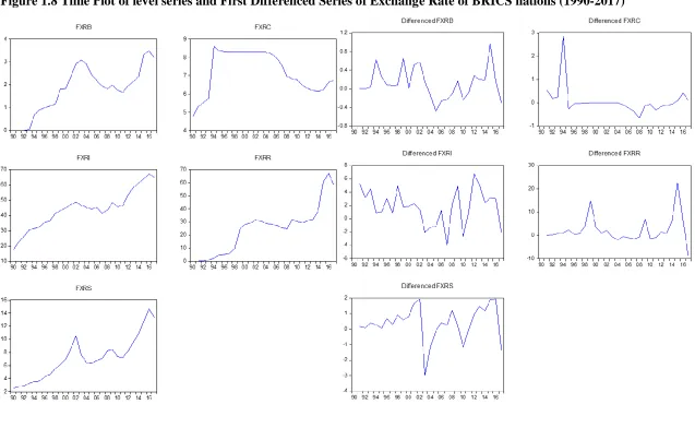
Figure 1.2 & 1.3 explain the trend line of foreign exchange rate in BRICS nations can be highlighted. The exchange rate was fluctuating between 1991 to 2018 for BRICS nations in terms of US dollars. India and Russia‟s currency continuously depreciated after 1990 in

comparison to that of China, Brazil and South Africa. The value of currencies of Brazil, Russia, India and South Africa have continuously deprecated against to US Dollar whereas only China‟s currency appreciated during the whole time period 1991-2017.

Figure 1.2 Trend of Exchange Rate in BRICS Nations

(18)

113

y = 0.092x - 183.9

R² = 0.532 _{y = 1.787x - 3557.}

R² = 0.772 y = 1.244x - 2448._{R² = 0.817}

y = -0.033x + 74.75

R² = 0.052 y = 0.304x - 602.6_{R² = 0.734}

0 20 40 60 80

1985 1990 1995 2000 2005 2010 2015 2020

foreign exchange rate

brazil russia india china south africa

Appreciation and Depreciation: Appreciation = (e1 - e0)/e0

Where e0 = old currency value, e1 = new currency value

Depreciation is the loss of value of a country's currency with respect to one or more foreign reference currencies, typically in a floating exchange rate system

1.9 Exchange Rate Determination in BRICS Nations: Time Series Analysis

The next step in the investigation of the evolution of the exchange rate volatility over time is testing the obtained volatility series for possible trends. To test the volatility series for potential trends three methods are used.

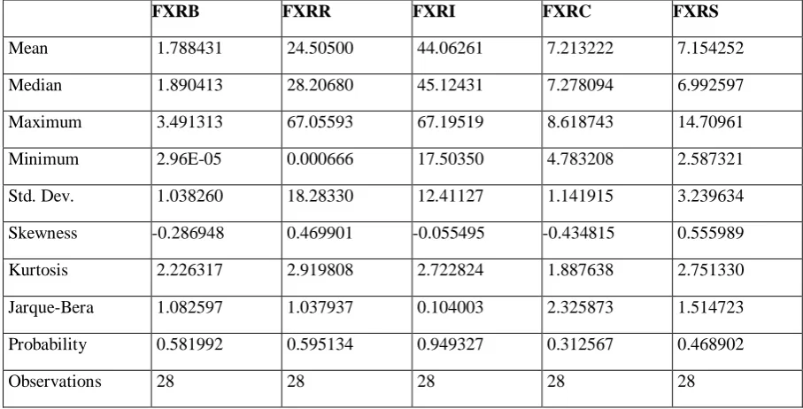
1. Descriptive Statistics Analysis

Table: 1.2 Descriptive Statistics Analysis

FXRB FXRR FXRI FXRC FXRS

Mean 1.788431 24.50500 44.06261 7.213222 7.154252

Median 1.890413 28.20680 45.12431 7.278094 6.992597

Maximum 3.491313 67.05593 67.19519 8.618743 14.70961

Minimum 2.96E-05 0.000666 17.50350 4.783208 2.587321

Std. Dev. 1.038260 18.28330 12.41127 1.141915 3.239634

Skewness -0.286948 0.469901 -0.055495 -0.434815 0.555989

Kurtosis 2.226317 2.919808 2.722824 1.887638 2.751330

Jarque-Bera 1.082597 1.037937 0.104003 2.325873 1.514723

Probability 0.581992 0.595134 0.949327 0.312567 0.468902

Observations 28 28 28 28 28

(19)

114

exchange rates for each individual currency against USD are BRL 1.78, RUB 24.50, INR 44.06,RMB 7.21, ZAR 7.15 respectively. The standard deviations of FXR is compared to the mean it shows that the values are far from the average which is an indication that the data sets of FXR have been tightly grouped. The coefficient of standard deviation are less in foreign exchange rate which indicates greater stability in this variable. The time series for FXR and price is negative skewed which indicate that large number of values below average value. Kurtosis value less than 3 which implies the FXR to be normally distributed.The Jarque-Bera shows that the series are all not normally distributed at one percent.The descriptive statistics results of the series in Russia. Exchange rate mean indicates that the value of Brazil‟s real on an average was 24.50 per US dollar. The standard deviations are positive in all series, indicating that FXR are volatile. These results indicate that international investors should expect the exchange rate to be highly volatile in the future (i.e. high appreciation or high depreciation of US Dollar) given the larger value of its excess kurtosis. The series exhibit skewness to the right, and the Jarque-Bera normality test suggests that all series are not normally distributed at the one percent level of significance. The descriptive statistics of the series in India. It suggests that all series are volatile, judging by the positive values of the standard deviations. All series are not normally distributed at one percent (rejecting the null hypothesis of being normally distributed at one percent) in India. The Jarque-Bera test for normality suggests that all series are normally distributed at one Percent for China and South Africa. RMB/US and Rand/US Dollar exchange rate both exhibit positive kurtosis with 1.88 and 2.75 respectively.

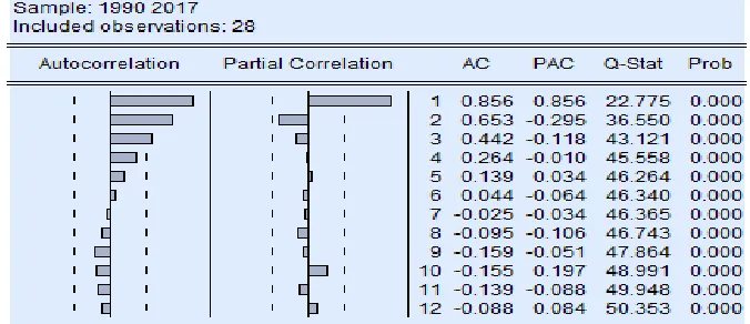
2. Unit root test for Data Analysis: On application of the Augmented Dicker Fuller Test on the level data, it was seen that the variables had a unit root or were not stationary. Subsequently, ADF was applied on the first difference of the series for each of the variables and the data was found to be stationary or having no unit root. Thus, the first difference of the series for each of the variables was computed. Thereafter the Johansen Cointegration test for the variables was conducted to check for cointegration amongst the variables. The assumption for Johansen cointegration test is that variables must be non-stationary or unit root at level series but after converting the variables into first difference they become stationary. The Johansen Cointegration showed that there is cointegration or long run association between the variables at 5% level. The guideline states that if variable are cointegrated then Vector Error Correction model should be run. However, if they are not cointegrated then VAR model should be run. Thus the Vector Error Correction model was run for the sample.

Table 1.3&1.4 before conducting any econometric analysis, the time series properties of the data must be investigated. This part of article, first conducts augmented Dickey–Fuller (1981) and Philip–Perron tests. The result are represent here the test for a unit root in the first difference series indicated strong rejection of the null hypothesis in all series. Then, all data series are integrated of order one. So, the first differencing, all the variables turn to out to be stationary. Figure 1.8, 1.9 &1.10 shows graphical representations of series at level and the first differenced stationary time series data and Autocorrelation testing at level and first

(20)

115

Table: 1.3 Results of ADF & Phillips -Perron Unit Root Tests on Exchange Rate of BRICS nations at level (1990-2017)

ADF critical value based on Mackinnon (1996) One-sided P-values (*1% **5% ***10%)

PP critical value based on Newey-West using Bartlett kernel (*1% **5% ***10%) SERIES IN LEVEL

VARIABLE Null Hypothesis: unit root ADF (t-Statistic)

(p-value)

PP Mac-Kinnon CRITICAL Value Result

Newey-West using Bartlett kernel

1% 5% 10%

FXRb Exogenous: Constant -1.796192 (0.3739)

-1.279571 (0.6240)

-3.711457 -2.981038 -2.629906 Non stationary I(0)

-3.699871 -2.976263 -2.62742

Exogenous: Trend and constant -2.138950 (0.5015)

-1.696290 ( 0.7250)

-4.356068 -3.595026 -3.233456 Non stationary I(0)

-4.33933 -3.587527 -3.22923

FXRr Exogenous: Constant -1.157782 (0.6766)

-0.407226 (0.8944)

-3.711457 -2.981038 -2.629906 Non stationary I(0)

-3.699871 -2.976263 -2.62742

-1.798176 (0.6775)

-4.356068 -3.595026 -3.233456 Non stationary I(0)

-4.33933 -3.587527 -3.22923

FXRi Exogenous: Constant -1.433936 (0.5508)

-1.411737 (0.5616)

-3.711457 -2.981038 -2.629906 Non stationary I(0)

-3.699871 -2.976263 -2.62742

-2.100555 (0.5224)

-4.356068 -3.595026 -3.233456 Non stationary I(0)

-4.33933 -3.587527 -3.22923

FXRc Exogenous: Constant -2.147617 (0.2290)

-2.337157 (0.1683)

-3.711457 -2.981038 -2.629906 Non stationary I(0)

-3.699871 -2.976263 -2.62742

-2.849679 (0.1932)

-4.356068 -3.595026 -3.233456 Non stationary I(0)

-4.33933 -3.587527 -3.22923

FXRs

Exogenous: Constant -0.396149 (0.8964)

-0.396149 (0.8964)

-3.711457 -2.981038 -2.629906 Non stationary I(0)

-3.699871 -2.976263 -2.62742

-1.793653 (0.6797)

-4.356068 -3.595026 -3.233456 Non stationary I(0)

(21)

116

Table:1.4 Results of ADF & Phillips -Perron Unit Root Tests on Exchange Rate of BRICS nations at First Differenced Series (1990-2017)

ADF critical value based on Mackinnon (1996) One-sided P-values (*1% **5% ***10%) PP critical value based on Newey-West using Bartlett kernel (*1% **5% ***10%)

Series in First Difference

VARIABLE Null Hypothesis: unit root

ADF (t-Statistic) (p-value)

PP

Mac-Kinnon CRITICAL Value

Result Newey-West using Bartlett kernel

1% 5% 10%

FXRb

Exogenous: Constant -3.416270** (0.0196)

-3.435242** (0.0188)

-3.711457 -2.981038 -2.629906 stationary I(1)

-3.699871 -2.976263 -2.62742

Exogenous: Trend and constant -3.364478*** (0.0783)

-3.378874*** (0.0762)

-4.356068 -3.595026 -3.233456 stationary I(1)

-4.33933 -3.587527 -3.22923

FXRr

Exogenous: Constant -4.177061* (0.0035)

-2.962416*** (0.0519)

-3.711457 -2.981038 -2.629906 _stationary I(1)

-3.699871 -2.976263 -2.62742

Exogenous: Trend and constant -4.032522** (0.0208)

-2.672342 (0.2548)

-4.356068 -3.595026 -3.233456 _stationary I(1)

-4.33933 -3.587527 -3.22923

FXRi

-4.033890* (0.0047)

-3.711457 -2.981038 -2.629906 stationary I(1)

-3.699871 -2.976263 -2.62742

-3.969452** (0.0231)

-4.356068 -3.595026 -3.233456 stationary I(1)

-4.33933 -3.587527 -3.22923

FXRc

-4.654448* (0.0010)

-3.711457 -2.981038 -2.629906 stationary I(1)

-3.699871 -2.976263 -2.62742

Exogenous: Trend and constant -4.970947* (0.0025)

-4.971036* (0.0025)

-4.356068 -3.595026 -3.233456 _stationary I(1)

-4.33933 -3.587527 -3.22923

FXRs

-3.614094** (0.0125)

-3.711457 -2.981038 -2.629906

stationary I(1)

-3.699871 -2.976263 -2.62742

-3.461115*** (0.0651)

-4.356068 -3.595026 -3.233456 stationary I(1)

(22)

117

(23)

118

http://ijmr.net.in, Email: [email protected] Figure1.9 Autocorrelation of Exchange Rate of BRICS nations (1990-2017)

- 1.0 - 0.5 0.0 0.5 1.0

2 4 6 8 10 12

Cor(F XRB, F XRB(-i))

- 1.0 - 0.5 0.0 0.5 1.0

2 4 6 8 10 12

Cor(F XRB, F XRC(-i))

- 1.0 - 0.5 0.0 0.5 1.0

2 4 6 8 10 12

Cor(F XRB, F XRI (-i))

- 1.0 - 0.5 0.0 0.5 1.0

2 4 6 8 10 12

Cor(F XRB, F XRR(-i))

- 1.0 - 0.5 0.0 0.5 1.0

2 4 6 8 10 12

Cor(F XRB, F XRS(-i))

- 1.0 - 0.5 0.0 0.5 1.0

2 4 6 8 10 12

Cor(F XRC, F XRB(-i))

- 1.0 - 0.5 0.0 0.5 1.0

2 4 6 8 10 12

Cor(F XRC, F XRC(-i))

- 1.0 - 0.5 0.0 0.5 1.0

2 4 6 8 10 12

Cor(F XRC, F XRI (-i))

- 1.0 - 0.5 0.0 0.5 1.0

2 4 6 8 10 12

Cor(F XRC, F XRR(-i))

- 1.0 - 0.5 0.0 0.5 1.0

2 4 6 8 10 12

Cor(F XRC, F XRS(-i))

- 1.0 - 0.5 0.0 0.5 1.0

2 4 6 8 10 12

Cor(F XRI , F XRB(-i))

- 1.0 - 0.5 0.0 0.5 1.0

2 4 6 8 10 12

Cor(F XRI , F XRC(-i))

- 1.0 - 0.5 0.0 0.5 1.0

2 4 6 8 10 12

Cor(F XRI , F XRI (-i))

- 1.0 - 0.5 0.0 0.5 1.0

2 4 6 8 10 12

Cor(F XRI , F XRR(-i))

- 1.0 - 0.5 0.0 0.5 1.0

2 4 6 8 10 12

Cor(F XRI , F XRS(-i))

- 1.0 - 0.5 0.0 0.5 1.0

2 4 6 8 10 12

Cor(F XRR, F XRB(-i))

- 1.0 - 0.5 0.0 0.5 1.0

2 4 6 8 10 12

Cor(F XRR, F XRC(-i))

- 1.0 - 0.5 0.0 0.5 1.0

2 4 6 8 10 12

Cor(F XRR, F XRI (-i))

- 1.0 - 0.5 0.0 0.5 1.0

2 4 6 8 10 12

Cor(F XRR, F XRR(-i))

- 1.0 - 0.5 0.0 0.5 1.0

2 4 6 8 10 12

Cor(F XRR, F XRS(-i))

- 1.0 - 0.5 0.0 0.5 1.0

2 4 6 8 10 12

Cor(F XRS, F XRB(-i))

- 1.0 - 0.5 0.0 0.5 1.0

2 4 6 8 10 12

Cor(F XRS, F XRC(-i))

- 1.0 - 0.5 0.0 0.5 1.0

2 4 6 8 10 12

Cor(F XRS, F XRI (-i))

- 1.0 - 0.5 0.0 0.5 1.0

2 4 6 8 10 12

Cor(F XRS, F XRR(-i))

- 1.0 - 0.5 0.0 0.5 1.0

2 4 6 8 10 12

(24)

119

Figure 1.10 Autocorrelation testing at level and first difference of Exchange Rate of BRICS nations (1990-2017)

Brazil

SERIES IN LEVEL SERIES IN FIRST DIFFERENCE

Russia

(25)

120

India

China

(26)

121

South Africa

3. Correlation Matrix Analysis

Table: 1.5 Correlation Matrix Analysis 1990-2017

FXRB FXRR FXRI FXRC FXRS

FXRB 1.000000 0.912707 0.887302 0.300950 0.881157

FXRR 0.912707 1.000000 0.939496 -0.016257 0.963110

FXRI 0.887302 0.939496 1.000000 0.071248 0.952800

FXRC 0.300950 -0.016257 0.071248 1.000000 -0.029922

(27)

122

To find the linear relationship between the study variables Karl Pearson‟s correlation test is applied. The result of correlation test is presented in Table 1.5 The relationship between the study variables is found to be positively and negatively correlated and significant at the 0.01 level. The results indicate that there is a positive highly correlation between FXR of brazil with FXR of Russia, India, China, South Africa but in Russia‟s FXR shows highly positive correlated with brazil, India south Africa and very low negative correlation with FXR of china. Also, it‟s observed FXR of India is high correlated with brazil, Russia and south Africa but low correlated with china and FXR of South Africa is the most least correlated variable with china. Thus China currency is less correlated with other BRICS nations.

4. COINTEGRATATION TEST:

Hypothesis 1. There is a co-integrating relationship among FXR

variables in BRICS nations

Johansen‟s cointegration test is applied to find stationary linear combination and long-run co-integrating equilibrium among the non-stationary variables. This test was introduced by Johansen (1988) and Johansen & Juselius (1991). The results of trace test and maximum eigenvalue test are presented in the table 1.6, it is clearly visible that for both the Trace Statistic as well as the Maximum Value Statistic, we find that there is no case where the null hypothesis (there is no cointegration among the variables) is rejected as the p-values are all greater than the critical value of 0.05.The table shows that first hypothesis i.e. no co integration among variables can be rejected as p-value (0.01%) is less than the critical value (69.81%) at 5% level of significance on the basis of trace statistics. The second null hypothesis i.e. there is at least one co integrating equation can be rejected because p-value is less than the critical vale at 5% level of significance, rather we reject this null hypothesis i.e. there is at least three co integrating equations. This implies that our variables are co integrated i.e. all the variables have long run association among them. And the Maximum Eigen test statistics makes the confirmation of this result.

Table: 1.6 Johansen Co-integration Test Results

Null Hypothesis Alternative Hypothesis

Trace Statistics

Critical Value5%

Prob.** MaxEigen value Critical Value5%

Prob.**

None * r=0 r>0 139.1474* 69.81889 0.0000 63.55363* 33.87687 0.0000 At most 1* r≤1 r≥1 75.59377* 47.85613 0.0000 35.02374* 27.58434 0.0046 At most 2 * r≤2 r≥2 40.57003* 29.79707 0.0020 25.21784* 21.13162 0.0125 At most 3 r≤3 r≥3 15.35219 15.49471 0.0525 14.25080 14.26460 0.0502 At most 4 r≤4 r≥4 1.101393 3.841466 0.2940 1.101393 3.841466 0.2940

1. Trace test indicates 3 cointegrating eqn(s) at the 0.05 level

(28)

123

http://ijmr.net.in, Email: [email protected] 5. Granger Causality analysis

Hypothesis 2. The exchange rate ﬂuctuations Granger-caused the foreign exchange rate of BRICS nations with each other. Table: 1.7 Granger Causality analysis (1990 to 2017)

Null Hypothesis: Obs F-Statistic Prob. Result (5% level of significance) Null Hypothesis:

Whole period (1990-2017)

FXRC does not Granger Cause FXRB 26 0.51538 0.6046 Accept FXR CHINA ---X---FXR BRAZIL DOES NOT CAUSE TO EACH OTHER FXRB does not Granger Cause FXRC 1.33366 0.2849 Accept

FXRI does not Granger Cause FXRB 26 3.67564* 0.0428 Reject FXR INDIA <=> FXR BRAZIL

INDICATES DUEL CAUSALITY BETWEEN BOTH

FXRB does not Granger Cause FXRI 3.69586* 0.0421 Reject

FXRR does not Granger Cause FXRB 26 0.37835 0.6896 Accept FXR RUSSIA ---X---FXR BRAZIL DOES NOT CAUSE TO EACH OTHER FXRB does not Granger Cause FXRR 0.04556 0.9556 Accept

FXRS does not Granger Cause FXRB 26 2.14574 0.1419 Accept FXR SOUTH AFRICA ---X---FXR BRAZIL DOES NOT CAUSE TO EACH OTHER FXRB does not Granger Cause FXRS 0.00057 0.9994 Accept

FXRI does not Granger Cause FXRC 26 1.32591 0.2869 Accept FXR INDIA---X---FXR CHINA DOES NOT CAUSE TO EACH OTHER FXRC does not Granger Cause FXRI 1.59015 0.2275 Accept

FXRR does not Granger Cause FXRC 26 1.59726 0.2261 Accept FXR RUSSIA ---X---FXR CHINA DOES NOT CAUSE TO EACH OTHER

FXRC does not Granger Cause FXRR 0.40638 0.6712 Accept

FXRS does not Granger Cause FXRC 26 0.90236 0.4208 Accept FXR SOUTH AFRICA ---X---FXR CHINA DOES NOT CAUSE TO EACH OTHER FXRC does not Granger Cause FXRS 0.55558 0.5819 Accept

FXRR does not Granger Cause FXRI 26 0.54910 0.5855 Accept FXR RUSSIA <= FXR INDIA

INDICATES UNIDIRECTIONAL CAUSALITY BETWEEN BOTH (ONE WAY CAUSALITY)

FXRI does not Granger Cause FXRR 9.88766* 0.0009 Reject

FXRS does not Granger Cause FXRI 26 1.03205 0.3737 Accept FXR SOUTH AFRICA <= FXR INDIA

INDICATES UNIDIRECTIONAL CAUSALITY BETWEEN BOTH (ONE WAY CAUSALITY)

FXRI does not Granger Cause FXRS 7.22068* 0.0041 Reject

(29)

124

After analysing that there is significant co integration in the sample series we estimate the Granger causality test to know the causality between the two variables. The results of Pair-wise Granger causality test done for 2 Time lags between the two variables for which unit root test is carried out. Granger causality test is used in this study to determine the causality between the study variables i.e. to check whether one variable is useful in forecasting the other variable and also helps in determining the short-run equilibrium relationship. For instance: variable X might „Granger cause‟ variable Y if past values of variable X explain variable Y. Similarly, variable Y „Granger causes‟ variable X, if past values of variable Y explain variable X. The results of Granger causality test are presented in Table 1.7.The results indicate that there is causality between the study variables. The direction of causality is found to be bidirectional (from fxr India fxr brazil and also from fxr India → fxr brazil) significant at 5% level. the results further indicate that there is one way causality between fxr Russia <= fxr India and fxr south Africa <= fxr India.

6. The impulse response

and variance decomposition

Hypothesis 4. The variance decomposition and impulse response among them are signiﬁcant

(30)

125

Figure1.11 Impulse Responses Testing of Exchange Rate of BRICS Nations (1990-2017)

- .2 .0 .2 .4 .6

2 4 6 8 1 0

Response of F XRB t o F XRB

- .2 .0 .2 .4 .6

2 4 6 8 1 0

Response of F XRB t o F XRR

- .2 .0 .2 .4 .6

2 4 6 8 1 0

Response of F XRB t o F XRI

- .2 .0 .2 .4 .6

2 4 6 8 1 0

Response of F XRB t o F XRC

- .2 .0 .2 .4 .6

2 4 6 8 1 0

Response of F XRB t o F XRS

- 2 0 2 4 6

2 4 6 8 1 0

Response of F XRR t o F XRB

- 2 0 2 4 6

2 4 6 8 1 0

Response of F XRR t o F XRR

- 2 0 2 4 6

2 4 6 8 1 0

Response of F XRR t o F XRI

- 2 0 2 4 6

2 4 6 8 1 0

Response of F XRR t o F XRC

- 2 0 2 4 6

2 4 6 8 1 0

Response of F XRR t o F XRS

- 1 0 1 2 3 4

2 4 6 8 1 0

Response of F XRI t o F XRB

- 1 0 1 2 3 4

2 4 6 8 1 0

Response of F XRI t o F XRR

- 1 0 1 2 3 4

2 4 6 8 1 0

Response of F XRI t o F XRI

- 1 0 1 2 3 4

2 4 6 8 1 0

Response of F XRI t o F XRC

- 1 0 1 2 3 4

2 4 6 8 1 0

Response of F XRI t o F XRS

- .8 - .4 .0 .4 .8

2 4 6 8 1 0

Response of F XRC t o F XRB

- .8 - .4 .0 .4 .8

2 4 6 8 1 0

Response of F XRC t o F XRR

- .8 - .4 .0 .4 .8

2 4 6 8 1 0

Response of F XRC t o F XRI

- .8 - .4 .0 .4 .8

2 4 6 8 1 0

Response of F XRC t o F XRC

- .8 - .4 .0 .4 .8

2 4 6 8 1 0

Response of F XRC t o F XRS

- 0 .4 0 .0 0 .4 0 .8 1 .2

2 4 6 8 1 0

Response of F XRS t o F XRB

- 0 .4 0 .0 0 .4 0 .8 1 .2

2 4 6 8 1 0

Response of F XRS t o F XRR

- 0 .4 0 .0 0 .4 0 .8 1 .2

2 4 6 8 1 0

Response of F XRS t o F XRI

- 0 .4 0 .0 0 .4 0 .8 1 .2

2 4 6 8 1 0

Response of F XRS t o F XRC

- 0 .4 0 .0 0 .4 0 .8 1 .2

2 4 6 8 1 0

(31)

126

The impulse response functions and their one-standard-deviation confidence bands are computed and drawn in Figure 1.11.

7. Variance Decomposition:

While impulse response functions trace the effects of a shock to one endogenous variable on other variables in then VAR, the alternative variance decomposition technique measures the proportion of forecast error variance in one variable explained by innovations in itself and the other variables. Thus, from the VDC, we can measure the relative importance of fluctuation of say, nominal or real shocks to variations in real exchange rate.

Table: 1.8 Variance Decomposition analysis

Variance Decomposition of FXRB:

Period S.E. FXRB FXRR FXRI FXRC FXRS

1 0.380439 100 0 0 0 0

2 0.641676 92.82792 0.573764 3.369131 0.00701 3.222178

3 0.866255 88.56897 1.552927 5.938659 0.004826 3.934621

4 1.05463 86.81199 2.169229 7.941335 0.008509 3.068935

5 1.190769 85.76171 2.237319 9.550205 0.01418 2.436582

6 1.302178 84.67552 2.228412 10.92624 0.032108 2.137728

7 1.398261 83.66621 2.21106 12.00257 0.034721 2.085446

8 1.487432 83.03936 2.138915 12.77837 0.031257 2.012102

9 1.576214 83.06985 2.025811 13.05115 0.027951 1.825243

10 1.665604 83.40301 1.901232 13.03049 0.027958 1.637305

Variance Decomposition of FXRR:

1 5.149299 75.7504 24.2496 0 0 0

2 9.503014 54.46607 27.67119 3.204121 0.069068 14.58956

3 12.78501 39.40832 30.91984 6.530732 0.213431 22.92768

4 15.04414 34.58199 33.61249 8.97165 0.56673 22.26714

5 16.34661 35.17188 35.04398 9.475388 0.7549 19.55386

6 17.37395 37.14572 35.23622 9.377903 0.716248 17.52391

7 18.45845 37.80157 35.53462 9.341836 0.641348 16.68063

8 19.75029 36.2859 35.92357 9.70604 0.589152 17.49534

9 21.01066 34.5717 36.3952 10.20982 0.626199 18.19708

10 22.00833 34.32791 36.79572 10.43451 0.70681 17.73505

Variance Decomposition of FXRI:

1 3.237307 23.54211 12.92646 63.53143 0 0

2 5.168539 27.47227 20.97454 51.34562 0.20677 0.000805

3 6.364636 25.37671 19.04487 55.08564 0.181465 0.311316

4 7.282707 22.14808 17.2421 58.83608 0.139143 1.634607

5 8.065576 20.85567 16.01879 60.47317 0.114384 2.537987

(32)

127

7 9.336746 19.19492 14.27653 63.44984 0.08689 2.991822

8 9.938284 19.04101 13.72498 64.01054 0.077523 3.145954

9 10.51613 19.10269 13.19115 64.18652 0.069289 3.450345

10 11.06957 19.15138 12.7662 64.32841 0.06365 3.690362

Variance Decomposition of FXRC:

1 0.74474 9.37114 76.54062 1.394936 12.6933 0

2 1.085923 12.52465 62.30985 13.41178 11.56728 0.186435

3 1.388237 15.41589 53.06015 20.1487 10.96162 0.413632

4 1.663978 16.33387 48.63719 24.36409 10.1475 0.517358

5 1.9196 15.87523 47.29792 25.98011 9.695884 1.150851

6 2.16378 15.96618 46.4223 26.27403 9.397691 1.939806

7 2.386699 16.17244 45.9207 26.17828 9.299124 2.429458

8 2.58783 16.19995 45.49746 26.50404 9.296052 2.502503

9 2.769291 16.1573 45.06079 27.0826 9.254725 2.444584

10 2.940395 16.12546 44.74231 27.52129 9.154204 2.456728

Variance Decomposition of FXRS:

1 1.223208 39.55336 16.1339 3.919051 0.512526 39.88116

2 2.106053 40.65432 25.8492 2.681585 0.340201 30.4747

3 2.537337 34.362 29.95812 6.544423 0.235367 28.90009

4 2.923758 28.15511 33.85796 9.366636 0.179574 28.44073

5 3.212387 24.35667 35.9733 10.44894 0.164399 29.05668

6 3.406791 22.15279 36.91165 11.25661 0.158973 29.51998

7 3.570216 21.36938 37.74022 11.42854 0.155547 29.30632

8 3.731238 21.46179 38.28926 11.27558 0.144553 28.82882

9 3.909697 21.21402 38.6522 11.23871 0.132681 28.76239

10 4.116918 20.34347 38.96562 11.34993 0.119679 29.22131

Cholesky Ordering: FXRB FXRR FXRI FXRC FXRS

(33)

DYNAMIC RELATIONSHIP BETWEEN EXCHANGE RATE OF BRICS COUNTRIES: CAUSALITY AND CO-INTEGRATION ANALYSIS

96

97

98

99

100

101

102

103

104

105

106

107

108









109

110

1.7 Model Specification for foreign exchange rate determination in BRICS

Nations:

111

112

113

foreign exchange rate

114

115

116

117

118

119

120

121

122

Hypothesis 1. There is a co-integrating relationship among FXR

variables in BRICS nations

123

124

6.

The impulse response

and variance decomposition

Hypothesis 4. The variance decomposition and impulse response among them are signiﬁcant

125

126

127

128