I
DENTIFYING
H
EDONIC
M
ODELS
Ivar Ekeland
James J. Heckman
Lars Nesheim
THE INSTITUTE FOR FISCAL STUDIES
DEPARTMENT OF ECONOMICS
,
UCL
Identifying Hedonic Models
Ivar Ekeland, James J. Heckman and Lars Nesheim¤
December, 2001
Economic models for hedonic markets characterize the pricing of bundles of attributes and
the demand and supply of these attributes under di®erent assumptions about market structure,
preferences and technology. (See Jan Tinbergen, 1956, Sherwin Rosen, 1974 and Dennis Epple,
1987, for contributions to this literature). While the theory is well formulated, and delivers some
elegant analytical results, the empirical content of the model is under debate. It is widely believed
that hedonic modelsfit in a single market are fundamentally underidentified and that any empirical
content obtained from them is a consequence of arbitrary functional form assumptions.
The problem of identification in hedonic models is a prototype for the identification problem in a
variety of economic models in which agents sort on unobservable (to the economist) characteristics:
models of monopoly pricing (Michael Mussa and Sherwin Rosen, 1978; Robert Wilson, 1993) and
models for taxes and labor supply (James Heckman, 1974). Sorting is an essential feature of
econometric models of social interactions. (See William Brock and Steven Durlauf, 2001). In this
paper we address the sorting problem in hedonic models. Nesheim (2001) extends this analysis to
a model with peer e®ects.
In this paper we note that commonly used linearization strategies made to simplify estimation
and justify the application of instrumental variables methods, produce identification problems. The
hedonic model is generically nonlinear. It is the linearization of a fundamentally nonlinear model
that produces the form of the identification problem that dominates discussion in the applied
literature. Linearity is an arbitrary and misleading functional form when applied to empirical hedonic models.
Our research establishes that even though sorting equilibrium in a single market implies no
exclusion restrictions, the hedonic model is generically nonparametrically identified.
without exclusion restrictions. Multimarket data, widely viewed as the most powerful source of
identification, achieves this result only under implausible assumptions about why hedonic functions
vary across markets.
I. The Hedonic Model
For specificity, consider a static labor market setting. Firms and workers match on attributes
z. Matches are 1-1. P(z) is the earnings of a worker who supplies attributes z, and Ris unearned
income. P(z) is the hedonic function. U(c, z, A, µ) are preferences of workers where A represents
preference parameters common across persons and µ represents preference heterogeneity
parame-ters that di®er across people and c is consumption (c = P(z) +R). Given P(z), assumed twice
di®erentiable, we obtain the standard first order and second conditions for a maximum. There is a
parallel problem for profit maximizingfirms that have technologyF(z;º, B) where º is a vector of
technology parameters that vary across firms, and B is a common technology parameter. Strictly
interior solutions are assumed. For simplicity we assume that dim µ = dim º where “dim” is
dimension. Neitherµ norº are assumed to be observable to the economist.
Under standard assumptions, we may invert the first order conditions to obtain the implicit
functions that map unobservables to observables and common parameters,µ=µ(z, Pz, P(z)+R, A)
andº =º(z, Pz, B), wherePz is the partial derivative ofP(z). Substituting into the densities forµ
and º we obtain the celebrated Rosen (1974) - Tinbergen (1956) equilibrium condition for hedonic
markets thatP(z) is the solution to a second order partial di®erential equation that equates demand
and supply densities at each point ofzin which a market operates. Under standard conditions, and
with su±cient boundary conditions, P(z) is uniquely determined from the equilibrium conditions.
II. A Linear - Quadratic Example
Assume preferences are quadratic in zand that dim (z) = dim (µ) :
U(c, z, µ, A) =R+P(z) +µ0z¡1 2z
0Az.
The conditions determining a consumer maximum setµ¡Az+Pzto zero and imply that (Pzz0¡A)
dim (z) = dim (º). Profits are
¦ (z, º, B, P(z)) =º0z¡1 2z
0Bz¡P(z)
and the conditions determining afirm’s optimum setº¡Bz¡Pzto zero and imply that¡(B+Pzz0)
is negative definite. The distributions ofº, µin the population are normal. The distribution ofµis
µsN(µµ; §µ), and the distribution of º is ºsN(µº; §º).
The price function induces a density of demand and a density of supply at every locationz. The
equilibrium price function can be found by equating these densities at every point z and solving
the resulting di®erential equation. In the normal-linear-quadratic case, the solution to the problem
is quadratic in z:
P(z) =¼0+¼10z+
1 2z
0¼ 2z.
Assuming the price function is quadratic, the first order conditions for thefirm are:
Firm: º¡Bz¡¼1¡¼2z= 0 (1)
and for the consumer they are:
Consumer: µ¡Az+¼1+¼2z= 0. (2)
From the second order conditions,B+¼2 and A¡¼2 are positive definite. Thus we may solve
forzfrom (1) to obtainz= (B+¼2)¡1(º¡¼1) and from (2)z= (A¡¼2)¡1(µ+¼1). Note that once
we have solved for ¼1 and ¼2, these latter two equations define the equilibrium matching function
linking the characteristics of demanders (1) to those of suppliers (2). For eachz,this function is
(B+¼2)¡1(º¡¼1) = (A¡¼2)¡1(µ+¼1).
To characterize equilibrium, we must equate demand and supply. In this linear normal case, all that
is required is to equate mean demand to mean supply and the variances of supply to the variances
of demand. Rearranging terms, we obtain an explicit expression for¼1 in terms ofA, B,µº,µµ and
[(A¡¼2)¡1+ (B+¼2)¡1]¡1[(B+¼2)¡1µº¡(A¡¼2)¡1µµ] =¼1.
To determine¼2,compute the variances of demand and supply from (1) and (2) respectively to
obtain the equilibrium condition:
(B+¼2)¡1
X
º(B+¼2)
¡1 = (A
¡¼2)¡1
X
µ(A¡¼2)
¡1.
We pin down initial conditions using the restrictions that U ¸U¯, a reservation value, and profits
are positive (¦¸0). These imply ¼0= 0.
III. Identifying The Model
Following Rosen (1974), we consider the problem of using data from a single market in which
P(z) is available and there are no missing attributes. Using the first order conditions ((1) and
(2) in the linear-quadratic-normal example) he proposed a two step method for estimating both
preference and technology parameters. He did not consider direct estimation of production, profit
or preference functions, a source of information we consider in our companion paper. If there are
no missing attributes, one can recover the production function directly from data on inputs and
outputs using standard methods. Even if production (or profit) data are available, data on utility
are not, so the problem considered by Rosen remains for recovering the parameters of at least one
side of the market.
From our discussion of the linear - quadratic - normal case, the parameters ¼1 and ¼2 do not
directly identify either preference or technology parameters except when Pµ = 0 or Pº = 0
respectively. The pricing function combines parameters in a di±cult-to-interpret fashion.
The most direct approach to estimating the hedonic model would be to solve the second order
di®erential equation implied by equilibrium for P(z) in terms of the parameters of preferences,
technology and the distributions of tastes and productivity and to jointly estimate the demand
functions and supply functions and distributions of preference and technology parameters exploiting
all of the information in the equilibrium conditions including data on demand, supply and the
pricing function. That approach is computationally complicated and does not transparently deliver
Rosen suggested an intuitively plausible and computationally simpler two step estimation
pro-cedure that has been widely criticized. In step 1 of his propro-cedure, the analyst estimatesP(z) from
market data. In step 2, the analyst uses first order conditions in conjunction with the marginal
prices obtained from step 1 to recover preferences and technology respectively.
In the context of the linear-quadratic example, the first stage would be to estimate pricing
function P(z), recover ¼1 and ¼2, and form the marginal prices and then estimate the curvature
parameters of technology, and preferences using (1) and (2) respectively. Specifically, he proposed
to estimate Band the mean of º (µº) from the least squares regression
b
Pz(z) = ˆ¼1+ ˆ¼2z=µº +Bz+"º (3)
where"º =º¡µº, and “ˆ” denotes estimate. A parallel proposal for preferences estimatesA and
the mean of µ(µµ) from the regression
b
Pz(z) = ˆ¼1+ ˆ¼2z=µµ+Az+"µ (4)
where"µ =µ¡µµ. We assume thatµµ and µº are functions of regressors (x) and (y) respectively,
µµ(x) andµº(y).
In an influential paper, James Brown and Harvey Rosen (1982) analyze the regression method
based on this idea. These papers contain most of the main ideas in the empirical literature on
hedonics that emerged from Rosen’s paper. They interpret (3) and (4) as linearizedapproximations
to the general first order conditions for the model. The linear-quadratic-normal is the framework
in which these approximations are exact.
In this approximation interpretation, the distributions ofº and µ are kept in the background.
Standard linear econometric methods are applied to identify the parameters of (3) and (4) and
connections among the parameters of preferences, technology and the distributions of tastes and
productivity are not made explicit. Issues of identification are confused with issues of
estima-tion. Common to an entire genre of empirical economics, this literature focuses on finding “good
Starting from (3) and (4), Brown and Rosen (1982) make three points which have been reiterated
in the subsequent empirical literature.
Point One: Identification Can Only Be Obtained Through Arbitrary Functional Form
Assumptions
Since z is on both sides of (3) and (4), by a property of least squares, a regression using the
constructed price Pbz(z) = ˆ¼1+ ˆ¼2zas the dependent variable in (3) or (4) only identifies¼2 even if
µº orµµ are functions of regressors. In general, ¼2 does not identify any technology or preference
parameter. In the special cases where there is no variation in preference parameters µ or where
there is no dispersion inº, ¼2 identifies preference (A) or production parameters (B) respectively.
However, if the constructed price is a nonlinear function of z, this argument no longer holds.
The nonlinear variation in Pbz(z) gives an added piece of information which can help to identify
technology and preference parameters. This identification strategy works because it rules out
collinearity between z and Pbz(z), but such nonlinearity is widely viewed as an artificial source
of identification that is thought to be “arbitrary.” In our companion paper, we prove that this
nonlinearity is a generic property of equilibrium in the hedonic model.
Point Two: Endogeneity
Even if such “arbitrary” assumptions are made, so that we can use the nonlinearity inPbz(z) to
help identify the parameters and circumvent Point One, we still face standard endogeneity problems.
zis correlated with "º and "µ in (3) and (4) respectively. Moreover, exclusion restrictions from the
other side of the market cannot be justified. The equilibrium matching condition requires that
"º ="µ+ (A¡B)z+µµ(x)¡µº(y)
so that conditional on z there is a functional and statistical dependence connecting "µ, "º, z and
the regressors.2 Conditional on z, "º, "µ, x and y become stochastically dependent even if in the
underlying population initially they are mutually independent.
With data from a single market, one is forced to hunt for “clever” instruments with a
ques-tionable economic basis. Thus, even if “arbitrary” nonlinearities are invoked, standard instruments
instruments even though there are no exclusion restrictions.
Point Three: Use of Multimarket Data
Brown and Rosen (1982), Epple (1987) and Kahn and Lang (1988), change Rosen’s problem
and consider estimation of thefirst order conditions using multimarket data either across regions,
or across time in the same region. The motivation for this approach is that if preferences,
technol-ogy, and the distributions of tastes and productivities are the same across markets but for some
unspecified reason price functions are not, variation in the Pz(z) across markets serves to identify
preferences and technology. This source of identification is viewed as being more robust.
The problem with this identification strategy is that it is logically inconsistent. If preferences,
technology, and the distributions of tastes and productivities are the same across markets,
equilib-rium price functions must be as well. The strategy is apparently more robust because it is vague
about the source of variation that makes price functions di®er when preferences, technology, and the
distributions of tastes and technology are common across markets. Under suitable restrictions on
preferences and technology, this approach can be used to identify the preferences or technology on
one side of the market. If preferences are stable and the distributions of preferences across markets
are stable, but technologies are di®erent for exogenous reasons, then multimarket variation shifts
the hedonic function against stable preferences and identifies preference parameters. Switching the
roles of technology and preferences, multimarket data identifies technology and the distribution of
technology parameters. If common preference and technology parameters are identical across
mar-kets, but heterogeneity distributions are di®erent across marmar-kets, then preference and technology
parameters and the heterogeneity distributions can be identified.
Using All Of The Economics of The Model
These criticisms are symptoms of a deeper problem: all of the economic content of the hedonic
model is not being exploited. We argue that when it is exploited, the model is generically identified
even within a single market without having to invoke arbitrary functional forms. We develop this
point formally in our companion paper. Here we develop the intuition for it using the
Consider all of the economic implications of the linear-quadratic model - not just the first
order conditions (1) and (2). Any reasonable specification of the model requires that profits be
non-negative, that utilities exceed threshold reservation values and that firm marginal products be
non-negative while marginal utilities of consumers for disamenities be non-positive. Adopting all
of these restrictions eliminates Point One within the linear-quadratic example.
The linear-quadratic-normal model results in an equilibrium with a linear marginal price
func-tion. This equilibrium produces an econometric system that is not identified. (Brown-Rosen Point
One). In this example, it would be arbitrary and incorrect to impose that the marginal price
function is nonlinear. However, the linear-quadratic model in Section II is very special. It belongs
to a very small class of models that produce an equilibrium marginal price function that is linear.
In our companion paper, we prove as a special case of a more general theorem that there is an
open dense set of models surrounding the linear-quadratic models of Section II that do not produce
linear marginal price functions. In these models, it is not arbitrary to impose nonlinear marginal
price functions.
The normal-linear-quadratic example has a number of peculiarities. From (1) and (2), it is
evident that marginal products can become negative, and marginal disutilities of labor (z) can
become positive. Nothing restricts marginal prices to be non-negative or for the demands or
supplies of z to be non-negative.
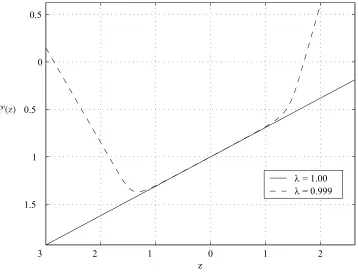
To see how fragile Point One is, suppose that we perturb a scalar version of the linear quadratic
model to have non-normal µ and º. The Figure shows the price functions for two cases. The
parameter values generating the Figure are given at the base. The first case is for º1 and µ1
normally distributed (¸ = 1; see the notes at the base of the Figure). The second case is for º1
andµ1 distributed as a mixture of normals with weights¸=.999 (on the original component which
produced the straight line) and 1¡¸=.001 (on the other component reported at the base of the
Figure). With this minor perturbation, the price function becomes highly nonlinear. The second
derivative of the price function is far from zero. A small dose of nonnormality produces a highly
These figures also reveal unattractive properties of the linear-quadratic model. Negative and
positive quantities of z are demanded and supplied and marginal prices are negative for a large
portion of the population. In our companion paper, we consider an example where marginal prices
are positive. In that case, marginal prices are nonlinear and positive and only positive quantities of
the amenity are demanded and supplied. By imposing economically plausible restrictions,
Brown-Rosen Point One is shown to be less cogent. In our companion paper, we show that these examples
are generic. They apply to a broad class of models with separable first order conditions and not
just linear-quadratic.
Even though Point One is non-generic, Point Two remains. There are apparently no valid
instruments for z on the right hand sides of (3) and (4). A strategy needs to be found to deal
with the endogeneity of z without exclusion restrictions.In our companion paper, we discuss two
such strategies based on transformation models and instrumental variables models and present
identification results for a general separable model with a single characteristic with no arbitrary
functional form restrictions or distributional assumptions and establish that the hedonic model
is generically identified from data from a single market. Intuitively, even though there are no
exclusion restrictions, instrumental variables is a valid estimator in a single market. In the context
of equations (3) and (4) one can show that E(z | x) and E(z | y) are not collinear with µµ(x)
and µº(y) respectively. Thus x and y are valid instruments (for supply and demand equations,
respectively) even though they are not excluded from their respective equations. See the proof in
Brock, William and Steve Durlauf. “Interactions Based Models,” in J. Heckman and
E. Leamer, editors, Handbook of Econometrics, Vol. 5. Amsterdam: North Holland, 2001, pp.
3297-3380.
Brown, James and Harvey Rosen. “On the Estimation of Structural Hedonic Price
Mod-els. Econometrica, 1982, 50, pp. 765-769.
Ekeland, Ivar, James J. Heckman and Lars Nesheim. “Identification and Estimation of
Hedonic Models”, University of Chicago, May 2001 revised November, 2001.
Epple, Dennis. “Hedonic Prices and Implicit Markets: Estimating Demand and Supply
Functions for Di®erentiated Products. Journal of Political Economy, 1987, 95 pp. 59-80.
Heckman, James. “The E®ect of Day Care Programs on Women’s Work E®ort.”
Journal of Political Economy, 1974, 82, pp 491-517.
Kahn, Shulamit and Kevin Lang. “E±cient Estimation of Structural Hedonic Systems,”
International Economic Review29 (1988): 157-166.
Mussa, Michael and Sherwin Rosen. “Monopoly and Product Quality.”
Journal of Economic Theory, 1978, 18, pp. 301-317.
Nesheim, Lars, “Equilibrium Sorting With Heterogeneous Agents: Theory and Empirical
Implications,” unpublished paper, UCL, London, 2001.
Rosen, Sherwin. “Hedonic Prices and Implicit Markets: Product Di®erentiation in Pure
Competition.” Journal of Political Economy, 1974, 82, pp. 34-55.
Tinbergen, Jan. “On The Theory of Income Distribution.” Weltwirtschaftliches Archiv ,
1956, 77 , pp. 155-73.
Footnotes
¤This research was supported by NSF 00-99195 and a grant from the American Bar Foundation.
Ekeland is at the University of Paris, Dauphine; Email: ([email protected]), Heckman is in the
Department of Economics at the University of Chicago, 1126 E. 59th Street, Chicago, IL 60637,
Telephone: (773) 702-0634, Fax (773) 702-8490, Email: [email protected]. Nesheim is at the
Institute for Fiscal Studies and the Department of Economics at UCL, London, England, Email:
1The model in this example was first analyzed by Tinbergen (1956) and has previously been
used by Epple (1987).
3 2 1 0 1 2 1.5
1 0.5 0 0.5
z
λ = 1.00
λ = 0.999 P'(z)
Figure 1
Slope of Price Function Legend:
a = 2, b = 1
Normal Linear Quadratic Model Mixture of Models
Normal Linear Quadratic Model (Tinbergen)
µν
1 = -1, σν1 = .3, µθ1 = .3, σθ1 = .5
2 2
Mixture of Normals Model
λ = .999 on Tinbergen Model components and λ = .001 on
µν
1 = -1, σν1 = .3, µθ1 = .3, σθ1 = .5