New algorithm for problems with exponential solutions

(1)

New algorithm for problems with exponential

solutions

A. O. Adesanya, R. O. Onsachi, M. R. Odekunle

Department of Mathematic, Modibbo Adama University of Technology, Yola, Nigeria

Abstract

In this paper, we consider the development of algorithms for the solution of …rst order initial value problems whose solution exhibits exponential behaviour. Method of interpolation and collocation of basis function to give system of nonlinear equa-tions which is solved for the unknown parameters to give a continuous scheme. The discrete methods recovered from the continuous scheme are implemented in block form. The stability properties of the method is veri…ed and numerical experiments show that our method is e¢ cient in handling these problems.

Key words: Exponentially-…tted method, interpolation, collocation, stability properties, continuous method, sti¤ problems

AMS subject classi…cation: 65L05, 65L06

1 Introduction

In this paper, we develop an exponentially …tted two step, hybrid numerical integrator for initial value problems (IVPs) of …rst order di¤erential equations in the form

y0 =f(x; y); y(x0) =y0; a x b (1.1)

where y : [a; b] _! _Rm_, _f _{: [}_{a; b}_]

R ! Rm_{; m} = ₁ _{is continuousely di¤erentiable.} The Jacobian arising from (1:1)vary slowly and the eigenvalues have negative real part; moreover the solution is decaying or exhibit a pronuounced exponential behaviour.

Classical general purpose method developed using …nite power series basis function cannot produce satisfactory results due to the special nature of the problems. Such problems are found in the modeling of disease outbreak, war, radioactive decay, di¤usion process in biology and chemical reactions. Several scholars have developed exponentially …tted methods are the best methods for(1:1)among them are [1–8] .

Corresponding author

(2)

The paper is organize as follows: section 2 discusses mathematical background and spec-i…cation of the method. Section 3 discusses the stability properties of the developed block method which include convergence and stability region of the developed method. Numer-ical experiments are shown in section 4 and we concluded in section 5.

2 Methodology

We consider the approximate solution

y(x) = m X

j=0

ajxj + m X

j=1

bje x j

(2.1)

where aj and b’js are constants to be determined. We seek approximation at an equidistant set of points de…ned by the the integration interval a x0 < x1 < < xN 1 < xN b.

xn=x0+nh; n= 0;1; ; N 1; h= _Nb a₁ , N is a positive integer

Interpolating and collocating(2:1) atxn+i; i= 0;1; ; k 1;give

XA =U (2.2)

where

A= a0 a1 a2 ak 1

T

U = yn yn+1 yn+r fn fn+1 fn+s T

X =

2 6 6 6 6 6 6 6 6 6 6 6 6 6 6 6 4

1 xn x2n xkn 1 e xn e x

2

n _e xkn

..

. ... ... ... ... ... ... ...

1 xn+r x2n+r xkn+1r e xn+r e x 2

n+r e xkn+r

0 1 2xn (k 1)xnk 2 e xn 2xne x

2

n kx

ne x k n

..

. ... ... ... ... ... ... ...

0 1 2xn+s (k 1)xnk+2s e xn+s 2xn+se x 2

n+s kx

n+se x k n+s

3 7 7 7 7 7 7 7 7 7 7 7 7 7 7 7 5

k=r+s 1: We then impose the following condition on y(x)in (2:1)

y(xn+i) = yn+i; i= 0;1 ; r; y0(xn+i) = fn+i; i= 0;1; ; s (2.3)

whererandsare the numbers of interpolation and collocation points respectively. Solving (2:2)using Crammer’s rule, substituting the result into (2:1) and after some algebraic simpli…cations gives the continuous method which when evaluated at selected grid points gives discrete methods.

In this paper, we consider interpolation atx=xnand collocation atx=xn+i; i= 0;1₂;1;2. Solving the resulting systems of equation gives the continuous method

(3)

0

=

1 2 2 e6 6 6 6 6 4

h + e 2 h 2 e

3h2

e h 2t 2 e h e h 2t 2 e 2 h + 2 e h 2t 2 e 3h2

2 he h 2 4 he 4 h 2 + 6 he

9h4

2 6 h 2 te 2 h h 2 + 12 h 2 te h 4 h 2 +8 h 2 te

3h2

h

2

8

h

2 te

3h2

4 h 2 12 h 2 te h

9h4

2 + 6 h 2 te 2 h

9h4

2 + 2 he h 2 e ht + 4 he 4 h 2 e ht 6 he

9h4 2 e ht + 2 h 2 t 2 e 2 h h 2 4 h 2 t 2 e h 4 h 2 2 h 2 t 2 e

3h2

h 2 + 4 h 2 t 2 e

3h2

4 h 2 + 3 h 2 t 2 e h

9h4

2 3 h 2 t 2 e 2 h

9h4

2

3 7 7 7 7 7 5

h h 3 e 2 h h 2 6 e h 4 h 2 4 e

3h2

h

2

+

4

e

3h2

4 h 2 + 6 e h

9h4

2

3

e

2

h

9h4

2 + e h 2 + 2 e 4 h 2 3 e

9h4

2

i

1

=

1 2

2 6 4

e h 2t 2 + 3 e 2 h 4 e

3h2

3 e h 2t 2 e 2 h + 4 e h 2t 2 e 3h2

12 he 4 h 2 + 12 he

9h4

2 + 12 he 4 h 2 e ht 12 he

9h4 2 e ht + 12 h 2 te 4 h 2 12 h 2 te

9h4

2 + 4 h 2 t 2 e

3h2

4 h 2 3 h 2 t 2 e 2 h

9h4

2 4 h 2 t 2 e 4 h 2 + 3 h 2 t 2 e

9h4

2

+

1

3 7 5

h h 3 e 2 h h 2 6 e h 4 h 2 4 e

3h2

h

2

+

4

e

3h2

4 h 2 + 6 e h

9h4

2

3

e

2

h

9h4

2 + e h 2 + 2 e 4 h 2 3 e

9h4

2

i

2

=

2 e6 4

h 2t 2 + 2 e h e 2 h 2 e h 2t 2 e h + e h 2t 2 e 2 h 4 he h 2 + 4 he 4 h 2 + 4 he h 2 e ht 4 he 4 h 2 e ht + 4 h 2 te h 2 4 h 2 te 4 h 2 + h 2 t 2 e 2 h h 2 2 h 2 t 2 e h 4 h 2 h 2 t 2 e h 2 + 2 h 2 t 2 e 4 h 2 1

3 7 5

h h 3 e 2 h h 2 6 e h 4 h 2 4 e

3h2

h

2

+

4

e

3h2

4 h 2 + 6 e h

9h4

2

3

e

2

h

9h4

2 + e h 2 + 2 e 4 h 2 3 e

9h4

2

i

3

=

1 2

2 e6 4

h 2t 2 + 3 e h 2 e

3h2

3 e h 2t 2 e h + 2 e h 2t 2 e 3h2

6 he h 2 + 6 he

9h4

2 + 6 he h 2 e ht 6 he

9h4 2 e ht + 6 h 2 te h 2 6 h 2 te

9h4

2

+2

h

2 t

2 e

3h2

h 2 3 h 2 t 2 e h

9h4

2 2 h 2 t 2 e h 2 + 3 h 2 t 2 e

9h4

2

1

3 7 5

h h 3 e 2 h h 2 6 e h 4 h 2 4 e

3h2

h

2

+

4

e

3h2

4 h 2 + 6 e h

9h4

2

3

e

2

h

9h4

2 + e h 2 + 2 e 4 h 2 3 e

9h4

(4)

3 Stability properties

De…nition 3.1 If we associate the linear operator `(y(x) :h) with the method (2:4) de-…ned by

`(y(x) :h) =yn+t yn 0fn+ 1fn+1+ 2fn+3₂ + 3fn+2 (3.1)

where y(x) is continuously di¤erentiable of[a:b]: Writing(3:1)as a Taylor series

expan-sion about x to obtain

`(y(x) :h) =c0y(x) +c1hy0(x) + +cphpy(p) (x) +

where the constant coe¢ cientcp; p= 0;1: are given as

`(y(x) :h) = 1 p!

X

jp _j 1

(p 1)! X

jp 1 _j 1

(p 1)! X

pj 1 _j !

then, (3:1)has order p if

`(y(x) :h) =O hp+1 ; c0 =c1 = cp = 0; cp+1 6= 0

cp+1 is the error constant and the local truncation error(LT E) =cp+1hp+1y(p+1)

Table 1: Order and LTE

t Order LTE

1 4 ₁₅2h5 159y000

n 4yn5

10 795h6 ₅₀₄₀_h5₊₉₈₅₆_h4₊₃₁₆₈_h3 ₇₁₆₈_h2₊₁₅₃₆

3

2 4

2

15h

5 52y000n 534y

5 n

10 795h6 ₅₀₄₀_h5₊₉₈₅₆_h4₊₃₁₆₈_h3 ₇₁₆₈_h2₊₁₅₃₆

2 4 ₁₅2h5 748y000

n 128y5n

10 795h6 ₅₀₄₀_h5₊₉₈₅₆_h4₊₃₁₆₈_h3 ₇₁₆₈_h2₊₁₅₃₆

De…nition 3.2 Method (2:4)is consistent if: (i) limh!0 yn+t_h yn = tyn0 (ii) it has order (p) 1

De…nition 3.3 A method is said to be zero stable if limh!0(yn+t)!yn

De…nition 3.4 A Method is said to be convergent if it is consistent and zero stable.

De…nition 3.5 The Region of absolute stability (RAS) of a method is the set

f h:for that h where the root of the stability polynomial are absolute less than one_g

In this paper, the boundary locus method is used to plot RAS. This is done by substituting the test equationy0 = y into the equation to obtain

h=z = (r)

(r)

(5)

0 0.05 0.1 0.15 0.2 0.25 0.3 0.35 0.4 0.45 -2.5

-2 -1.5 -1 -0.5 0 0.5 1 1.5 2 2.5

Real

Im

agi

nary

RAS

Fig 1: Region of absolute stability of the method

4 Numerical examples

The e¢ ciency of the developed method is tested using …ve test problems withn= 300

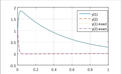
Problem 4.1 We consider the linear system in the range 0 x 1

y0 = 0 B

@ 1 95

1 97

1 C

Ay; y(0) = 0 B

@1

1 1 C A

Source: [2]. The eigenvalues of the Jacobian matrix are 1 = 2; 2 = 96 with the

sti¤-ness ratio 48. The exact solution is given asy(x) = 1

47(95e

2x ₄₈_e 95x_;₄₈_e 96x _e 2x₎T_.

(6)

0

0.2

0.4

0.6

0.8

1 -0.5

0

0.5

1

1.5

2

y(1) y(2) y(1) exact y(2) exact

Fig. 2: Results of problem 4.1

x values

0

0.2

0.4

0.6

0.8

1 lo

g

(e

rr

o

r)

-8

-6

-4

-2

0

y(1) y(2)

Fig. 3: Log(error) against x values for problem 4.1

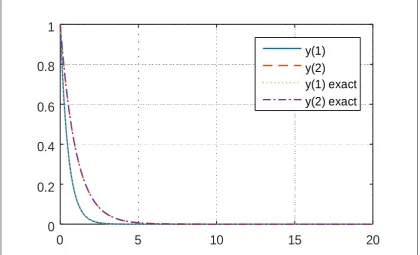
Problem 4.2 We consider a non-linear system in the range 0 x 20

0 B

@y

0

1(x)

y₂0 (x) 1 C

A=

0 B

@ 1002y1(x) + 1000y

2

2(x)

y1(x) y2(x) (1 +y2(x))

1 C

A;

0 B

@y1(0)

y2(0)

1 C

A=

0 B

@1

1 1 C A

with exact solution(y(x)) = (exp ( 2x); exp ( x))T :

(7)

0

5

10

15

20

0

0.2

0.4

0.6

0.8

1 x values

0

5

10

15

20 lo

g

(e

rr

o

r)

-25

-20

-15

-10

-5

0

y(1) y(2)

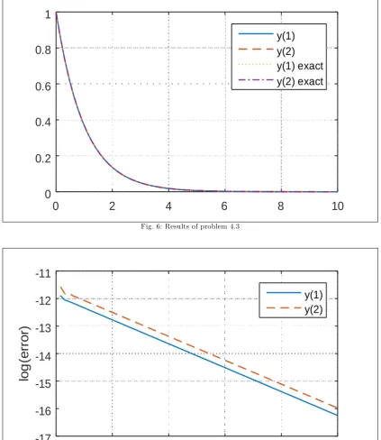
Problem 4.3 Consider a system in the range0 t 10

y0 = 0 B

@ 1 30

30 1

1 C

Ay+

0 B

@ 30e

t

30e t 1 C

Ay; y(0) = 0 B

@1

1 1 C A

with exact solutiony(x) = (e t; e t)T

(8)

0

2

4

6

8

10

0

0.2

0.4

0.6

0.8

1 x values

0

2

4

6

8

10 lo

g

(e

rr

o

r)

-17

-16

-15

-14

-13

-12

-11

y(1) y(2)

Problem 4.4 consider the sti¤ system in the interval 0 t 5

0 B

@y

0

1

y₂0 1 C

A=

0 B

@ 1001y1+ 999y2+ 2y1y2 999y1 1001y2 +y21+y22

1 C

A;

0 B

@y1(0)

y2(0)

1 C

A =

0 B

@ 0

1 1 C A

with the exact solutiony(x) = ₂₀₀₁1000_e2000t ₁

1

3e2t ₁;

1000 2001e2000t ₁

1

3e2t ₁

T

:

(9)

0

1

2

3

4

5 -1

-0.8

-0.6

-0.4

-0.2

0 x values

0

1

2

3

4

5 lo

g

(e

rr

o

r)

-8

-6

-4

-2

0

y(1) y(2)

Problem 4.5 consider the simple nonlinear sti¤ problem within the interval x= [0;20]

0 B

@y

0

1

y0

2

1 C

A=

0 B

@ y1

2y2

1 2y2

1 C

A;

0 B

@y1(0)

y2(0)

1 C

A=

0 B

@5

5 1 C A

with the exact solutiony(x) = (5e x_; ₅_e 2x_{(1 + 5}_x₎₎T _:

(10)

0

5

10

15

20

0

2

4

6

8 x values

0

5

10

15

20 lo

g

(e

rr

o

r)

-20

-15

-10

-5

0

y(1) y(2)

5 Conclusion

(11)

References

[1] G. V. Berghe, H. D. Meyer, M. V. Daele, T. V. Hecke. Exponentially …tted Runge Kutta method. Journal of Computational and Applied Mathematics, 125(2000),107-115

[2] C. E. Abdulimen. Exponentially …tted third derivative three step method for numerical integration of sti¤ initial value problems. Applied Mathematics and Computation, 243, (2014), 446-453

[3] Y. Fengjian, C. Xinming, L. Yiping. High order one step A-stable exponentially …tted method. Appl. Math. J. Chiness Univ. Ser. B. 14(3), (1999), 357-365

[4] T. E. Simon. Exponentially-…tted Runge Kutta- Nystrom method for the numerical solution of initial value problems with oscillating solutions. Applied Mathematics Letters. 15, (2002), 217-225

[5] T. Y. Ying, N. Yaacob. One step exponentially-rational method for the numerical solution of …rst order initial value problems. SIAM Malaysiana, 42(6), (2013), 845-853

[6] J. Carroll. A matricial exponentially …tted scheme for the numerical solution of sti¤ initial value problems. computers. Math. Applic. 26(4), (1993), 57-64

[7] Y. Yang, Y. Fang, X. You, B. Nang. Novel exponentially …tted two derivative Runge Kutta methods with equation-dependent coe¢ cient for …rst order di¤erential equations. Discrete Dynamics in Nature and Society. doi:org=10:1152=2016=9827952

[8] A. Xiao, G. Zhang, X. Yi. Implicit-explicit multistep method for nonlinear sti¤ initial value problems. applied Mathematics and Computations, 247, (2014), 47-60

[9] S. O. Fatunla. Nonlinear multistep methods for initail value problems. Comp. & Maths. with Appls. 8(3), (1993) 231-239

[10] D. G Yakubu, S. Markus. The e¢ ciency of second derivative multistep methods for the numerical integration of sti¤ systems. Journal of the Nigerian Mathematical Society, (2016).