Models Trained Bigrams Tested Bigrams bigram model (the, ball), (a, naughty), (naughty, boy) (the, tennis), (tennis, ball), (a, boy) skip-bigram model (the, ball), (a, naughty), (naughty, boy),(a, boy) (the, tennis), (tennis, ball),(a, boy) proposed model (the, ball),(a, boy), (boy, naughty) (ball, tennis),(the, ball),(a, boy)
Table 1: An example of bigrams trained and tested by three different kinds of models. The bolded bigrams occur in both training data and test data.
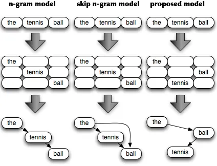
Figure 1: The assumptions of three different models
B is in the training data and A is in the test data, then the bigrams (the, tennis), (tennis, ball) and trigrams (hit, the, tennis), (the, tennis, ball) cannot be learned too. Besides, the skipping is actually a partial enu-meration of word combinations, which come along with lots of modeling redundancy.
Since ’tennis ball’ is a specification of pattern ’... ball’, it is more appropriate to consider that ’tennis’ depends upon ’ball’ rather than its preceding word ’the’. Similarly, ’the ball’ can be considered as a specification of pattern ’the ...’. Based on such an assumption, we propose to reorder the dependent se-quence as ’the!ball!tennis’ instead of the origi-nal one (’the!tennis!ball’), and consequently, the bigrams are trained and tested as (the, ball), (ball, tennis), which is quite different from the traditional sequential way as shown in Figure 1.
To reveal the advantages of this idea, suppose we have {’the ball’, ’a naughty boy’} in the
train-ing data and{’the tennis ball’, ’a boy’} in the test data. Table 1 shows what we will have in the bi-gram model and the skip-bibi-gram model, and what we hope to have in our proposed model. As shown in this table, our model learns pairs of words that
hopefully have direct dependencies. Besides, with-out enumeration, proposed model can keep size of trained grams as small as normal n-gram model.
Although we also change the word sequence of test data in a different way, it is still appropriate to compare it with n-gram models for two reasons. First, the word sequence of training data and test data are reordered by the same assumption that a word depends upon its schematic pattern as we de-scribed above, just as the n-gram model assume that every word of test data depends upon its preceding words. Second, the number of total tested bigrams is still the same as that of n-gram models. For each word of test data, we only make a different assump-tion about what the dependent words should be.
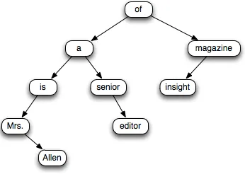
Since these dependent words can be determined if we parse ’the tennis ball’ into an intermediate struc-ture as shown in Figure 1, the only remaining prob-lem is how to achieve such kind of structure from any sequence. Although similar structures can be achieved by applying dependency parsers, the accu-racy of word dependency parsing is highly language-dependent. It is expected for us to figure out a method that can be applied to any language as easily as normal n-gram models.
Intuitively, the more frequently a word is used, the more probable it becomes part of a useful pattern. We establish our method based on such a heuristic rule in the following section.
3 Method
As we discussed previously, we assume that a word depends upon its schematic pattern, and also assume that such a pattern consists of relatively high fre-quency words.
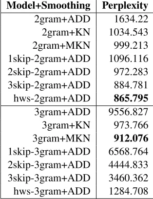
Model+Smoothing Perplexity 2gram+ADD 1634.22 2gram+KN 1034.543 2gram+MKN 999.213 1skip-2gram+ADD 1096.116 2skip-2gram+ADD 972.283 3skip-2gram+ADD 884.781 hws-2gram+ADD 865.795 3gram+ADD 9556.827 3gram+KN 973.766 3gram+MKN 912.076 1skip-3gram+ADD 6568.764 2skip-3gram+ADD 4444.833 3skip-3gram+ADD 3460.362 hws-3gram+ADD 1284.708
Table 3: Perplexity values of normal n-gram models, skip-n-gram models and proposed model by applying dif-ferent smoothing methods
& Ney,1995) and modified Kneser-Ney (Chen & Goodman,1999) as smoothing method separately.
P(wi|wii n1+1) = C(w i
i n+1) +↵
C(wi ni 1+1) +↵V
3 (1)
The results are shown in Table 3, since the grams of our model is trained in a special way, it’s not ap-propriate to directly incorporate lower order mod-els to higher ones, and consequently, we cannot di-rectly apply Kneser-ney Smoothing on our model4. Yet even though with additive smoothing, our bi-gram model outperforms normal bibi-gram model with Modified Kneser-Ney Smoothing. Thus, if we can figure out an appropriate way to incorporate it to our trigram model, it is highly possible that ours outper-forms normal trigram models as well.
4.3 Coverage and Usage
This experiment illustrates the coverage and usage of our model compared to those of normal n-gram model and skip-n-gram model. We trained on the entire BNC corpus (100 million words) and mea-3V stands for vocabulary size, and smoothing parameter
↵ (0.0001↵1.0) is determined by golden section search (Kiefer,1953).
4Neither can skip-n-gram model.
Figure 4: The coverage of 3-grams
Figure 5: The usage and F-Score of 3-grams
sured the coverage on 100,000 words of newswire from the Gigaword corpus.
We list all trigrams of test data to examine how many of them actually occurred in trained model and how many trigrams of trained model actually are used in test data.
We define the grams of training data as TR, and unique grams of test data as TE, then we calculate coverage by Equation 2.
coverage= |T R
T
T E|
|T E| (2)
We also use Equation 3 to estimate how much re-dundancy contained in a model and Equation 4 as a balanced measure.
usage= |T R
T
T E|
|T R| (3)
F Score= 2⇥coverage⇥usage
Figure 6: The growth of trained grams with the addition of training data size
Figure 7: The decreasing of usage with the addition of training data size
The results of coverage are shown in Figure 4. Even though skip-gram model use a partial enu-meration of word combinations to expand trained grams, proposed model still outperforms 3skip-3-gram model by 7.3 percent.
Figure 5 shows the results of usage and F-score. Apparently, there is much less modeling redundancy in our model, and as a result, ours keeps better bal-ance between coverage and usage than the other ones.
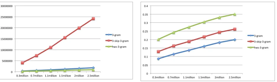
4.4 Length of Trained Grams and Training Data Size
This experiment examines the relation between length of trained grams and training data size. We use exactly the same test data (100,000 words of Gi-gaword corpus) as above. But for training data, we use different portions of different sizes of BNC cor-pus. We gradually increase the amount of training data to examine how it affects these trained grams.
Figure 8: The increasing of coverage with the addition of training data size
Intuitively, the length of trained grams will be in-creased with the addition of corpus size. As shown in Figure 6, in comparison with normal 3-gram model and hws-3-gram model, the grams learned by 3-skip-3-gram grow very fast, which means the cost of producing and storing them is quite considerable. Consequently, the growth of grams comes along with modeling redundancy, appearing as the de-creasing of usage. As shown in Figure 7, though hws-3-gram is decreasing, it is still more efficient (with higher usage) than the other two models.
Of course, the inefficiency of 3-skip-3-gram would be worth if it resulted in higher coverage. But as shown in Figure 8, all the three kinds of mod-els increase at almost the same speed, and proposed model still hold the lead.
5 Conclusions and Future Work
In this paper, we proposed a hierarchical word se-quence language model to make full use of contex-tual information and relieve the data sparsity prob-lem.
Proposed model has a good performance on de-creasing perplexity, which also keeps better balance between coverage and usage than normal n-gram model and skip-n-gram model. Besides, the cost of storing our model is more economical than other models.
trained by our model, some useful sentence patterns can be extracted, which is also a promising future study.
References
B. Allison, D. Guthrie, et. al. 2005.Quantifying the
Like-lihood of Unseen Events: A further look at the data Sparsity problem. Awaiting publication.
C. E. Shannon. 1948. A Mathematical Theory of
Com-munication. The Bell System Technical Journal, 27: 379-423.
D. Chiang. 2007. Hierarchical Phrase-based
Transla-tion. Computational Linguistics, Vol33, No.2, 201– 228.
D. Guthrie, B. Alliso, et. al. 2006. A Closer Look at
Skip-gram Modelling. Proceedings of the 5th international Conference on Language Resources and Evaluation, 2006: 1-4.
J. Kiefer. 1953. Sequential minimax search for a
maxi-mum. Proceedings of the American Mathematical So-ciety, 1953, 4(3): 502-506.
R. Kneser, H. Ney. 1995. Improved backing-off for
m-gram language modeling.Acoustics, Speech, and Sig-nal Processing, 1995. ICASSP-95., 1995 InternatioSig-nal Conference on. IEEE, 1995, 1: 181-184.
S. F. Chen, J. Goodman. 1999. An empirical study of
smoothing techniques for language modeling. Com-puter Speech & Language, 1999, 13(4): 359-393.
S. Katz. 1987. Estimation of probabilities from sparse
data for the language model component of a speech recognizer. Acoustics, Speech and Signal Processing, IEEE Transactions on, 1987, 35(3): 400-401.
X. Huang, F. Alleva, H. W. Hon, et al. 1993. The
SPHINX-II speech recognition system: an overview.